Social Networks and Choice Set Formation in Discrete Choice Models

Abstract

The discrete choice literature has evolved from the analysis of a choice of a single item from a fixed choice set to the incorporation of a vast array of more complex representations of preferences and choice set formation processes into choice models. Modern discrete choice models include rich specifications of heterogeneity, multi-stage processing for choice set determination, dynamics, and other elements. However, discrete choice models still largely represent socially isolated choice processes —individuals are not affected by the preferences of choices of other individuals. There is a developing literature on the impact of social networks on preferences or the utility function in a random utility model but little examination of such processes for choice set formation. There is also emerging evidence in the marketplace of the influence of friends on choice sets and choices. In this paper we develop discrete choice models that incorporate formal social network structures into the choice set formation process in a two-stage random utility framework. We assess models where peers may affect not only the alternatives that individuals consider or include in their choice sets, but also consumption choices. We explore the properties of our models and evaluate the extent of “errors” in assessment of preferences, economic welfare measures and market shares if network effects are present, but are not accounted for in the econometric model. Our results shed light on the importance of the evaluation of peer or network effects on inclusion/exclusion of alternatives in a random utility choice framework.

1. Introduction

The task of modeling individuals’ choices is definitely an ambitious one. Decisions are influenced by numerous factors that range from the number of alternatives and attributes like price and quality, to a more complex set of drivers like social norms, social pressure, and levels of scrutiny and anonymity. In addition, the structure of the decision making process itself may be complex and require different stages, e.g., a choice set formation (CSF) stage before a decision making stage.

A stylized fact emerging from various literatures on consumer choice suggests that when facing a large number of alternatives, consumers tend to screen options and reduce the set they actually consider to a small fraction of those available. Hauser et al. [1] suggest that in automobile choice, consumers in the U.S. consider only 10 of the more than 350 make and model combinations available to them. In the case of consumer packaged goods (deodorants, detergents, etc.) a review by Hauser [2] states that consumers typically consider only 10% of the available brands and that knowledge of the consumer’s choice or consideration set can vastly improve forecasting of choice. The marketing literature has provided ample empirical evidence corroborating the existence of “consider-then-choose” processes (van Nierop et al. [3]). A consider-then-choose two step decision making approach can be viewed as an efficient response to information processing costs and choice complexity (Hauser [2]). Various researchers also suggest that the focus of advertising is to influence the consumer’s consideration set (e.g., getting a consumer to test drive an automobile or at least include the make-model in their small set of cars to consider).

While there is evidence supporting relatively small consideration or choice sets, a key question is how the choice set is formed. Consider-then-choose models can be thought of as models of bounded rationality where consumers do not automatically consider all options and marketing is a tool for influencing choice set formation (Eliaz and Spiegler [4]). A variety of forms of benefit-cost mechanisms have been proposed including the use of heuristics or screening rules to reduce search or cognitive costs (Hauser [2]). In the case of automobiles, evaluating all makes and models would be extremely time consuming and complex and even selecting those to test drive can be a challenging task. The literature abounds with sets of rules or strategies that appear to be used by consumers including utility based screening (passing a certain utility threshold) or heuristics such as the construction of lists of requirements (“must have”) or features that result in rejection from a choice set (Hauser [2]; Swait and Erdem [5]).

An emerging factor in choice set formation is the influence of reviews (e.g., Consumer Reports) and the influence of “friends.” According to the Forbes Magazine, modern consumers (or “millennials”, individuals born after 1980) rely on the feedback of their peers before making a purchase (Forbes [6]). Consider the context of automobile choice. A recent report from AutoTrader.com${}^{\copyright }$, one of the largest online auto purchasing entities, states that millennials are emerging as automobile purchasers now that they are finishing college and earning incomes. This group of individuals, however, appear to rely much more on online reviews of products, and are heavily influenced by their friends or peer-group. According to AutoTrader [7] this group is much more likely to use word-of-mouth to develop consideration sets and choose cars. A recent blog post quotes the North American CEO of the auto manufacturer BMW as saying “Millennials choose vehicles by relying on word of mouth, recommendations from friends and influencers”, …“As I speak, we are developing programs to leverage key influencers who already have thousands of millennial followers” (Automotive News [8]).

In terms of studying consumer choice, the challenge then becomes how to incorporate the influence of friends into the choice process. It may be that friends influence the perception of attributes or the quality of features such as comfort, reliability, ease of handling, etc. Alternatively it could be that friends influence the choice set by suggesting brands or makes/models to consider. Given the large number of attributes that characterize an automobile, it would seem likely that friends would play at least as large a role in influencing choice set formation as they would influence perceptions of individual attributes. In addition to friends, consumers making automobile choices also appear to rely heavily on reviews or consumer reports—which can be viewed as a grouping of trusted individuals. This group may also influence choice set formation, or attribute perception, or both.

In this paper we construct formal models of social influence on choice and examine the impact of such influence on both choice set formation and a consumer’s utility function (affecting attribute perceptions). More specifically, we assess the impact of ignoring such processes on econometric results and consumer welfare and market shares measurement. While our models are generic they will apply to cases like automobile choice, consumer packaged goods, selection of restaurants, recreation site choice, and a host of other categories where consumers are expected to use a consider-then-choose strategy. Our econometric approach employs discrete choice models with foundations in random utility maximization (RUM) to explain choices. These models have been used in transportation economics, health economics, environmental economics, industrial organization, and other subfields of economics. As interest in explaining choices has increased, RUM theory and empirical application has evolved.

The discrete choice model literature has progressed to develop models to accommodate complex decision-making processes. For example, the literature evolved from simple binary choice models to models that consider (ordered and unordered) multiple discrete choices (see Zavoina and McKelvey [9] and McFadden [10] for examples of ordered and unordered models, respectively). The literature has also evolved from considering single decision processes (choice of an alternative from a fixed set of alternatives) to models that incorporate different stages of the choice process (see Swait and Ben-Akiva [11] for an example of two-stage consider-then-choose discrete choice model). Correctly specifying CSF has been shown to be very important in parameter estimation and economic welfare measurement (see for example, Li et al. [12]; Swait and Erdem [5]; Bierlaire et al. [13]).

The discrete choice literature has focused on choice behavior of self-interested and socially isolated individuals. Economic theory has evolved to develop models that consider a broader range of determinants of behavior like impure altruism (Andreoni [14]), fairness (Rabin [15]), morality (Levitt and List [16]), social networks (Neilson and Wichmann [17]), to name a few. The empirical literature has evolved to provide support for these behaviors. For instance, Duflo and Saez [18] show that the decision to participate in retirement plans is influenced by peers’ choices; and Chowdhury and Jeon [19] report results of a laboratory experiment that supports predictions of the impure altruism theory.

As a range of factors and processes is involved in explaining choices, estimates from empirical methods that fail to accommodate such complexity may significantly misrepresent true parameters. Moreover, economic welfare estimates based on misspecified discrete choice models can seriously mislead policy. As a result, there is a large and long-standing methodological literature that constantly evolves in an attempt to make econometric models more flexible and able to deliver more reliable estimates. In the context of incorporating social networks or peer effects into discrete choice models, Brock and Durlauf [20] and Lee et al. [21] develop binary choice models in which the choice of an individual is influenced by his or her connected friends. Soetevent and Kooreman [22] develop an empirical discrete choice model of social interactions that is estimated by means of simulation methods. Richards et al. [23] examine how the network centrality of an individual influences the product choices of others. Wichmann [24] outlines the implications of ignoring social network influences on the utility component of discrete choice models.

As mentioned above, this paper focuses on the role of social networks in the choice set formation stage. It contributes to the discrete choice literature by developing a two-stage discrete choice model in which, in the first stage, individuals’ social networks influence the formation of their choice sets and, in the second stage, individuals choose an alternative from their respective choice sets to maximize their utilities. Specifically, the paper’s starting point is a standard two-stage independent availability logit (IAL) model (see Manski [25]; Swait [26]; Swait and Ben-Akiva [11,27]). In the model, choice set formation is a probabilistic process characterized by a quality cutoff, i.e., low quality alternatives are not considered for choice by the individual. We build on the IAL model by assuming that the probability that an alternative is included in an individual’s choice set is a function not only of her own perception about the alternative’s quality but also a function of the quality perception of the individual’s social network. We also examine a framework where social networks influence perceptions in the utility function in addition to the CSF process.

We propose a CSF process in which overall quality perception is a convex combination of own and network perceptions such that the network may increase or decrease socially isolated (or private) quality perception. The weight of social network quality on overall quality perception is captured by a parameter denoted as degree of social interaction in CSF. Members of a social network with high degree of social interaction place more weight on their social connections’ quality perception than on their own perception. This weighing mechanism guarantees that the network model nests the standard IAL model, i.e., when the degree of social interaction is equal to zero (no social interaction) the network does not play a role in CSF and the model collapses to the basic IAL model. Similarly, we consider a model in social network quality may affect choice with the strength determined by a parameter denoted as degree of social interaction in choice.

Through a series of Monte Carlo experiments, we investigate the consequences of estimating two-stage IAL models that ignore the effects of social networks on CSF when the underlying data generating process (DGP) is influenced by social connections. The experiments vary the degrees of social interactions of the DGP. For each replication, in each experiment, we obtain two sets of maximum-likelihood estimates: one based the correctly specified network model and one based on the misspecified IAL model that ignores social networks.

Not surprisingly, we find that the empirical distributions of the estimates of the network models are centered on their true values confirming consistency. These models deliver precise estimates with proportional root mean square errors generally below 5%. We find that empirical distributions of IAL estimates are generally centered around their true values when network effects are weak. When network effects are moderate or strong, estimates of the standard IAL model present large biases and their distributions are extremely wide making estimates very imprecise.

We also use Monte Carlo experiments to examine the bias of the IAL model on estimating the effect of a hypothetical project that increases the quality of one alternative. We estimate welfare impacts of the project (a public policy perspective, e.g., improving the quality of a public park) and the effect of the project on market shares (a private firm perspective, e.g., altering quality perceptions through advertisement). While network models perform very well, we find that IAL estimates of the welfare impacts and market share gains can significantly underestimate the true impacts of the project. This downward bias increases with the degrees of social interactions and, when network effects are strong and operate through both CSF and choice channels, the IAL underestimates welfare and market share gains by approximately 190% and 77%, respectively.

The remainder of the paper is organized as follows. Section 2 presents two standard discrete choice models (Multinomial Logit and IAL) and their theoretical foundations. Section 3 builds on the standard models to develop our network models of CSF. Section 4 describes how to construct welfare measures from discrete choice model estimates. Section 5 introduces the Monte Carlo experiments and Section 6 presents the simulation results. Section 7 offers a discussion.

2. Unordered Multiple Choice and Choice Sets

The Multinomial Logit (MNL) model is perhaps the most prevalent model in the literature of unordered discrete multiple choice models. Its underlying fundamentals are established under random utility maximization theory. Typically, the random utility for individual n of choosing alternative j from a choice set B containing J alternatives is represented as $U_{nj}=V_{nj}+{\epsilon }_{nj}$, where $V_{nj}$ denotes systematic utility (i.e., deterministic utility that is influenced by observable characteristics), and ${\epsilon }_{nj}$ is a stochastic component reflecting unobservable individual and alternative specific heterogeneities. The random utility model postulates that alternative j will be chosen if and only if j is the alternative that provides the highest utility among all feasible alternatives. Formally, $U_{nj}\ge {\max }_{k\in B}{U}_{nk}$. The probability that subject n chooses alternative j is $P_n(j)=Prob\left(U_{nj}\ge \max (U_{nk})\right)$, or simply

$$P_n(j)=Prob(V_{nj}+{\epsilon }_{nj}\ge V_{nk}+{\epsilon }_{nk},\forall k\in B).$$

(1)

The MNL was developed by McFadden [10] by assuming that the disturbance ${\epsilon }_{nj}$ is independent and identically distributed (i.i.d.) and follows a Gumbel (Type I Extreme Value) distribution.1 Specifically, when $\epsilon \sim \mathbf{G}(0,1)$, where 0 is the location parameter and 1 is the positive scale parameter, the probability $P_n(j)$ in Equation (1) can be written as

$$P_n(j)=\frac{exp(V_{nj})}{{\displaystyle \sum _{k\in B}}exp(V_{nk})}.$$

(2)

$V_{nj}$ is often assumed to be a linear function of attributes of alternative j. Formally, $V_{nj}=V_n(x_j)=x_{nj}^{\prime }\beta$, where $x_{nj}$ is a vector of attributes of alternative j for individual n (e.g., price p and quality q) and β is a parameter vector. For each alternative, estimates of β, the probability of selection, and marginal effects, can be straightforwardly obtained using the maximum-likelihood (ML) method.

Note that the likelihood function of the MNL model depends on the correct specification of the choice set B. In the MNL model, each individual is assumed to face the same set of alternatives and this choice set is known with certainty by the econometrician. The MNL model ignores the fact that in reality different individuals may face different choice sets, and makes the (potentially problematic) simplifying assumption that there is an unique global choice set known by the econometrician. In some cases, the researcher defined choice set may include alternatives that are never considered by individuals (B would have too many alternatives). In other cases, some relevant alternatives may not be included in B (too few alternatives). In both cases, the likelihood function is misspecified and the MNL model will deliver biased estimates (Swait and Ben-Akiva [11,27]; Li et al. [12]).

It seems reasonable to expect that feasible choice sets are endogenously formed by individuals themselves rather than predetermined by researchers. These endogenous behaviors are called choice set formation (CSF) processes (Manski [25]) and normally are not observed by the econometrician. This unobservability suggests that choice set models should have probabilistic CSF processes.

The major breakthrough focusing on the CSF process is attributed to Manski’s [25] seminal study, where the author extended the MNL model into a separable two-stage consider-then-choose model. That is, in the first stage decision makers form a choice set and in the second stage they choose an alternative from this set. Manski’s formulation is the following. A population consisting of N decision makers face a primitive finite set B containing J alternatives.2 The CSF problem of individual n at the first stage is to draw a nonempty subset $C\subseteq B$. In a second stage, each decision maker chooses one alternative to maximize random utility. The random utility function, defined on the feasible set C (rather than B), provides RUM-consistency. The unconditional probability that alternative j is selected is written as

$$P_n(j)=\sum _{j\in C,C\subseteq B}{Q}_n(C)P_n(j\mid C),$$

(3)

where j is an alternative in C; $Q_n(C)$ is the probability that C is individual n’s true choice set; and $P_n(j\mid C)$ is the conditional probability that alternative j is chosen given that C is individual n’s true choice set.

Treatments of $P_n(j\mid C)$ are unanimously coherent throughout the literature and are consistent with McFadden’s [10] MNL model. $P_n(i\mid C)$ is defined as

$$P_n(j\mid C)=\left\{\begin{array}{cc}\frac{exp(V_{nj})}{{\displaystyle \sum _{k\in C}}exp(V_{nk})},\hfill & \mathrm{if}j\in C\hfill \\ 0,\hfill & \mathrm{if}j\notin C,\hfill \end{array}\right.$$

(4)

where $V_{nj}$ is the systematic utility term of $U_{nj}$. Specifically, as defined above, $U_{nj}$ takes the additive random utility form with

$$U_{nj}=V_{nj}+{\epsilon }_{nj}=x_{nj}^{\prime }\beta +{\epsilon }_{nj},$$

(5)

where ${\epsilon }_{nj}$ is i.i.d. Gumbel distributed with the scale parameter fixed at unity. Equation (4) differs from Equation (2) by assigning a zero probability when alternative j is not included in n’s choice set. This is possible because the two-stage model incorporates a CSF process that allows for alternatives to not be part of the decision maker’s true choice set.

The independent availability logit (IAL) model proposed by Swait [26] and Swait and Ben-Akiva [27] builds on Manski’s [25] two-stage choice paradigm by defining $Q_n(C)$ as

$$Q_n(C)=\frac{{\displaystyle \prod _{h\in C}}{A}_n(h){\displaystyle \prod _{k\in (B-C)}}[1-A_n(k)]}{1-{\displaystyle \prod _{j\in B}}[1-A_n(j)]},$$

(6)

where h, k and j are alternatives belonging to different choice sets as denoted in Equation (6), and $A(·)$ denotes the probability that an alternative is included in the corresponding choice set.3 The IAL model assumes independence from irrelevant alternatives (IIA) and therefore the choice probability ratio between two alternatives in C is independent of the inclusion/exclusion of an irrelevant alternative to/from C.

For individual n, $A_n(j)$ captures the availability of alternative j. As suggested by Swait and Ben-Akiva [27], $A_n(j)$ describes the aggregate impact of constraints on alternative attributes (for example, an external price constraint or a quality constraint imposed on public goods and services). These constraints may be also affected by individual specific tastes. In this paper, we assume the availability of an alternative is determined by a quality cutoff such that

$$A_n(j)=Prob(q_{nj}>{\tau }_0+{\xi }_{nj})=\frac{1}{1+exp[-\mu (q_{nj}-{\tau }_0)]},$$

(7)

where $q_{nj}$ is individual n’s perception about the quality of alternative j, ${\tau }_0$ is a quality threshold parameter; and ${\xi }_{nj}$ is an i.i.d. random variable that follows a logistic distribution with location of zero and scale of μ. One way to interpret the cutoff property of the availability function (7) is to read $A_n(j)$ as the probability that decision maker n’s quality perception about alternative j (i.e., the deterministic component of availability) is above a random quality threshold determined by ${\tau }_0+{\xi }_{nj}$.

Equations (3)–(7) define the IAL model. Parameter estimates are often obtained through maximum-likelihood estimation. This method has been applied in several disciplines for methodological and applied research. For instance, Chang et al. [32] use the IAL to evaluate the performance of hypothetical surveys and laboratory experiments in predicting actual field behavior. The IAL was also used in environmental economics, to estimate a random utility model of recreation demand (Haab and Hicks [33]); in transportation, for route choice modeling (Habib et al. [34]); and in marketing, to estimate consumer discrete choice using scanner data (Andrews and Srinivasan [35]).

3. Social Networks and Choice Set Formation

We propose two social network discrete choice models that are extensions of the IAL model. In our first model, social networks affect the formation of choice sets. In determining the availability of alternatives, we examine decision makers that not only consider their own perceptions about the quality of each alternative, but also the quality perception of those in their social networks. We introduce this feature in the IAL model by modifying the availability function. We refer to this model as the single network effect discrete choice model with choice set formation (SNE hereafter).

In our second model, social networks influence not only the formation of choice sets but also the utility that individuals receive from each alternative. Specifically, we consider a model in which an individual’s utility from alternative j is affected not only by attributes of j as perceived by the individual (e.g., own quality perception), but also by attributes of j as perceived by her social network (e.g., network quality perceptions). We refer to this model as the double network effect discrete choice model with choice set formation (DNE hereafter). The next section begins the exposition of our models by introducing our approach for representing social networks.

3.1. Modeling Social Networks

The paper uses the sociometric approach to model social networks. In this approach, social connections are captured through the rows of a matrix. Sociomatrices are a simple way to model networks with one dimension, and are well-suited for developing discrete choice models with network effects.4

Consider an environment in which N decision makers are connected in a social network. The network is represented by a $N\times N$ matrix A, where an element $a_{nm}=1$ if decision maker n is connected to decision maker m $(\forall n\ne m)$, and $a_{nm}=0$ otherwise. We assume the diagonal of A is equal to zero reflecting the fact that decision makers are not socially connected to themselves. We also assume that every decision maker has at least one connection.

The model does not impose symmetry of A. Decision maker n may be connected to m while m is not connected to n. This implies that A is a directed network. The relevance of this property will be evident in the next sections when we add social network effects into the IAL model. This property indicates that, if $a_{nm}=1$ and $a_{mn}=0$, decision maker m influences decision maker n, however, n does not influence m. Therefore, the n-th row of A represents n’s social connections, in other words, it indicates all decision makers with a social influence on n.

Let W be a row-normalization of A such that its elements are $w_{nm}=a_{nm}/{\sum }_m{a}_{nm}$. The n-th row of W represents a distribution of weights that the row decision maker assigns to the connections with the column decision makers. This normalization implies that all connections of a decision maker’s network have identical weight.5 However, our CSF model allows for respondents to adjust the relative strengths of own and network characteristics. This is described in the next section.

3.2. Social Network Effects on Alternative Availability

When studying a socially connected group of individuals, it is useful to use matrix notation to facilitate understanding of key modeling concepts. Let q be a $N\times J$ matrix representing the quality perception profile of the decision makers in the social network W. Its $(n,j)$ element $q_{n,j}$ is individual n’s quality perception about alternative j. The matrix Wq is therefore the quality profile of the decision makers’ social networks.6 We assume the deterministic component of availability to be a convex combination of own and network quality perceptions. Considering the entire network, this component can be written as

$$(1-{\tau }_1)\mathbf{q}+{\tau }_1\mathbf{W}\mathbf{q},$$

(8)

where ${\tau }_1\in [0,1]$ is a parameter denoted as degree of social interaction in choice set formation. It reflects the extent to which decision makers’ value their social network quality perceptions relative to their own.

Notice that, for decision maker n, the network component of availability is simply the average quality perceptions of n’s network (i.e., n-th row of Wq). The availability of alternative j to decision maker n is determined by comparing element $(n,j)$ of the matrix (8) with the random quality threshold determined by ${\tau }_0+{\xi }_{nj}$. Specifically, availability is probabilistically defined in our network model as

$$\begin{array}{cc}\hfill A_n(j)& =Prob\left((1-{\tau }_1)q_{nj}+{\tau }_1{\tilde{q}}_{nj}>{\tau }_0+{\xi }_{nj}\right)\hfill \\ & =\frac{1}{1+exp\left[-\mu \left(q_{nj}+{\tau }_1({\tilde{q}}_{nj}-q_{nj})-{\tau }_0\right)\right]},\hfill \end{array}$$

(9)

where ${\tilde{q}}_{nj}={\sum }_m{w}_{nm}{q}_{mj}$ and ${\xi }_{nj}$ is a logistic distribution with location equal to zero and scale equal to μ.

The availability function (9) incorporates social network effects on the probability that an alternative is included in respondents’ choice sets. When ${\tau }_1$ is high, there is a high degree of social interaction in choice set formation and a large weight is assigned to network perception and a low weight is assigned to own perception. When ${\tau }_1=0$, decision makers are socially isolated in terms of deciding availability, the network is irrelevant for the CSF process, and the model collapses into the standard IAL model (see Equation (7)).

The network model imposes a trade-off between the relevance of own and network quality perceptions to the CSF process. This is important to allow for the social network to increase or decrease the likelihood that an alternative is part of one’s choice set. When the quality of alternative j perceived by decision maker n ($q_{nj}$) is smaller than the average quality perception of n’s network (${\tilde{q}}_{nj}$), the network effect increases the probability that j is included in n’s choice set when compared to the probability assigned by model (7). On the other hand, when own quality perception is greater than network perception, the social network decreases the likelihood of the alternative being part of the choice set.

An intuitive way to interpret these network effects is to assume that decision makers have their own (or prior) opinions about the quality of the alternative, however, they consult their networks to update their quality perceptions. The extent to which the network will affect (either positively or negatively) the probability of availability depends on the degree of social interaction in choice set formation. When ${\tau }_1$ is high, we expect a large difference between the probabilities assigned by functions (7) and (9). When ${\tau }_1$ is close to zero, this difference is expected to be small.

Equation (9), together with Equations (3)–(6), completely describe the SNE model of discrete choice. Estimates of the utility parameters β and the CSF parameters ${\tau }_0$ and ${\tau }_1$ can be obtained through maximum-likelihood estimation.

3.3. Social Network Effects on Availability and Utility

This section presents the DNE model in which social networks affect not only the availability of alternatives, i.e., Equation (9), but also the utility that individuals receive from each alternative. As before, we assume that the systematic part of utility $V_{nj}$ is a linear function of $x_{nj}=(x_{1nj},...,x_{Knj})$, the vector of K attributes of alternative j for individual n. However, we assume that utility has two components: one represents attributes of alternative j as perceived by individual n, captured by $x_{nj}$, the other represents attributes of alternative j as perceived by n’s social network, captured by ${\tilde{x}}_{nj}=({\sum }_m{W}_{nm}{x}_{1mj},...,{\sum }_m{W}_{nm}{x}_{Kmj})$, where m indexes individuals represented in the columns of matrix W. As a result, the DNE model replaces utility (5) with

$$U_{nj}=V_{nj}+{\epsilon }_{nj}={\alpha }_0+x_{nj}^{\prime }{\beta }_{\mathrm{OWN}}+{\tilde{x}}_{nj}^{\prime }{\beta }_{\mathrm{NET}}+{\epsilon }_{nj},$$

(10)

where ${\alpha }_0$ is an intercept and ${\epsilon }_{nj}$ is i.i.d. Gumbel distributed with the scale parameter fixed at unity.

Conceptually, this utility formulation is consistent with numerous strategic game-theoretic models. For example, in auction theory, interdependent values models are auction models where bidders have different information about the value of the good being auctioned, and a bidder’s valuation of the good depends not only on his own signal about the value, but also on information about others’ signals (see Milgrom and Weber [40]; Eso and White [41]).

The peer effect identification literature refers to the coefficient ${\beta }_{\mathrm{NET}}$ as contextual effects, or exogenous social effects (see Manski [42]). These network effects have been shown to influence students’ participation in recreational activities (Bramoulle et al. [43]) and academic achievement (Lin [44]). Moreover, Patacchini and Venanzoni [45] show that the demand for housing quality is affected not only by education but also by network education.

Equations (3), (4), (6), (9) and (10), completely describe the DNE model of discrete choice. All parameters can be estimated through maximum-likelihood.

We finalize this section with three remarks. First, note that the SNE model is a special case of the DNE model in which ${\beta }_{\mathrm{OWN}}=\beta$ (from Equations (5) and (10), respectively) and ${\beta }_{\mathrm{NET}}=0$. Second, note that the utility (10) can be re-arranged as

$$U_{nj}={\alpha }_0+\left((1-{\alpha }_1)x_{nj}^{\prime }+{\alpha }_1{\tilde{x}}_{nj}^{\prime }\right)\beta +{\epsilon }_{nj},$$

(11)

where, ${\alpha }_1\in [0,1]$ is a scalar and, for each variable in $x_{nj}$, ${\beta }_{\mathrm{OWN}}=(1-{\alpha }_1)\beta$ and ${\beta }_{\mathrm{NET}}={\alpha }_1\beta$. One can think of β as the combined effect of own and network influence, and ${\alpha }_1$ as the degree of social interaction in choice, i.e., the share of the combined effect of $x_{nj}$ on utility that comes from network (as opposed to own) perceptions of $x_{nj}$. The combined effect β can be estimated as $\widehat{\beta }=\left({\widehat{\beta }}_{\mathrm{OWN}}+{\widehat{\beta }}_{\mathrm{NET}}\right)$, and the degree of social interaction in choice can be estimated as ${\widehat{\alpha }}_1={\widehat{\beta }}_{\mathrm{NET}}/\left({\widehat{\beta }}_{\mathrm{OWN}}+{\widehat{\beta }}_{\mathrm{NET}}\right)$. Inference on these parameters can be based on standard errors obtained through the delta method. Third, note that the IAL model is a special case of the DNE models as the DNE collapses to the standard IAL when agents are socially isolated in choice set formation and in choice, i.e., ${\tau }_1=0$ and ${\alpha }_1=0$.

4. Estimation of Welfare Impacts

This section derives welfare measures for discrete choice models with choice set formation. Our exposition follows the notation of the DNE model, however, as the SNE and the IAL models are special cases of the DNE, the material in this section applies to the three models.

We consider a framework in which the utility that decision maker n receives from alternative j is a function of its price (p), own quality perception (q), and network quality perception ($\tilde{q}$).7 Our interest is to evaluate the welfare generated by a project that changes the level of one attribute of alternative j. As such, we consider a project that increases the quality of alternative j. Assuming that decision maker n chooses alternative j (before and after the project), n’s compensating variation ($CV$) for this project is determined by

$$U(p,q^1,{\tilde{q}}^1,y-CV)=U(p,q^0,{\tilde{q}}^0,y),$$

(12)

where the superscript 1 refers to the quality of the alternative induced by the project (i.e., quality after the project), the superscript 0 is the status quo quality (before the project), p denotes price, and y denotes income.8 As utility is increasing in quality and income, $CV$ will be positive. It captures the income reduction that makes the decision maker indifferent between the project and the status quo scenarios. In fact, $CV$ is the decision maker’s willingness to pay for the quality enhancement project.

As previously discussed, it is common to specify a linear functional form for representative utility. Equation (12) can therefore be re-written as

$${\beta }_y(y-p-CV)+{\beta }_{\mathrm{OWN}}{q}^1+{\beta }_{\mathrm{NET}}{\tilde{q}}^1+\epsilon ={\beta }_y(y-p)+{\beta }_{\mathrm{OWN}}{q}^0+{\beta }_{\mathrm{NET}}{\tilde{q}}^0+\epsilon ,$$

(13)

where ${\beta }_y$, ${\beta }_{\mathrm{OWN}}$, and ${\beta }_{\mathrm{NET}}$ are parameters of the utility function. Note that ${\beta }_y$ is the marginal utility of income, or the marginal disutility of a price increase. Therefore ${\beta }_y=-{\beta }_{price}$.

Notice that we must adapt the standard welfare measurement approach to a probabilistic model of utility. Decision maker n obtains random utility $U_n=V_n+{\epsilon }_n$ from choosing only one alternative from his choice set (where ${\epsilon }_n$∼$\mathbf{G}(0,1)$). Hence, the $CV$ measure must be defined in equilibrium because individuals only obtain utility from the chosen alternative. $CV$ must compare the maximum U under the project against the maximum U under status quo. Ben-Akiva and Lerman [28] (pp. 104–106) describe properties of the Gumbel distribution that allows for the specification of $CV$ in this setting. Decision maker n’s random utility $V_n+{\epsilon }_n\sim \mathbf{G}(V_n,1)$. It follows that $\max (V_{n1}+{\epsilon }_{n1},V_{n2}+{\epsilon }_{n2},...,V_{nJ}+{\epsilon }_{nJ})\sim \mathbf{G}(\ln {\sum }_{j\in B}exp(V_{nj}),1)$. Therefore, the expected value of $V_{nj}^{*}=\max (V_{nj}+{\epsilon }_{nj})$ is $\ln {\sum }_{j\in B}exp(V_{nj})$. Applying these concepts to Equation (13) leads to $CV=\frac{1}{{\beta }_y}[V^{*}(q^1)-V^{*}(q^0)]$ and expected $CV$ equal to

$$\begin{array}{cc}\hfill E[CV]& =\frac{1}{{\beta }_y}[\ln \sum _{j\in B}exp(V_j^1)-\ln \sum _{j\in B}exp(V_j^0)]\hfill \\ & =\frac{1}{{\beta }_y}[\ln \sum _{j\in B}exp(x_j^1\beta )-\ln \sum _{j\in B}exp(x_j^0\beta )],\hfill \end{array}$$

(14)

where $x_j^1$ and $x_j^0$ are attribute levels after and before the policy change and β are the linear utility parameters.

Note that the process of deriving Equation (14) has an underlying assumption that all alternatives are available to the decision maker (i.e., there is a global choice set B as in the standard MNL model).9 In the IAL model (with or without social networks), the choice sets are formed probabilistically. Since changes in expected maximum utility are choice-set-specific, the welfare should be weighted by the corresponding choice set probabilities. Specifically,

$$E{[CV]}_{IAL}=\frac{1}{{\beta }_y}\{\sum _{C\subseteq B}[Q{(C)}^1\ln \sum _{i\in C}exp(x_i^1\beta )]-\sum _{C\subseteq B}[Q{(C)}^0\ln \sum _{i\in C}exp(x_i^0\beta )]\},$$

(15)

where $Q{(C)}^1$ and $Q{(C)}^0$ are the probability of choice set C being the true choice set after and before the policy change, respectively. This welfare measure depends not only on utility parameters β, but also on CSF parameters ${\tau }_0$ (and also ${\tau }_1$ in the network model). Estimates of welfare are obtained by substituting (maximum-likelihood) estimates of the parameters into Equation (15).

5. Monte Carlo Experiments

Current applications of the IAL model do not account for social network effects on choice set formation. By proposing an IAL models with social networks, our paper provides a benchmark to evaluate IAL estimates that ignore social networks when networks are part of the data generating process (DGP). In such a situation, the IAL model is misspecified and its estimates are (theoretically) biased. The goal of the paper’s experiments is not only to confirm the existence and measure the magnitude of this bias but also, and most importantly, to explore possible correlations between social structure (as captured by the degree of social interaction in CSF and choice) and the bias.

Our experimental design is summarized in

Table 1. Summary of experimental design.

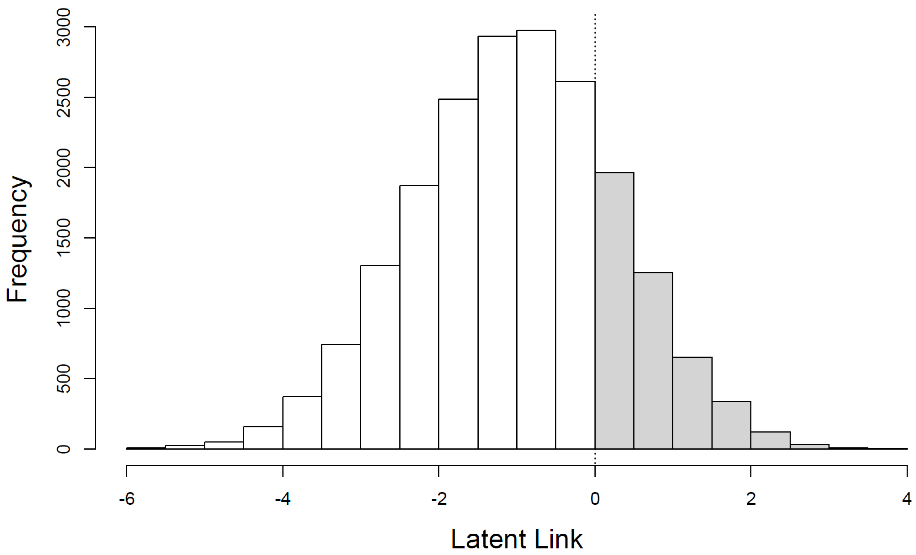
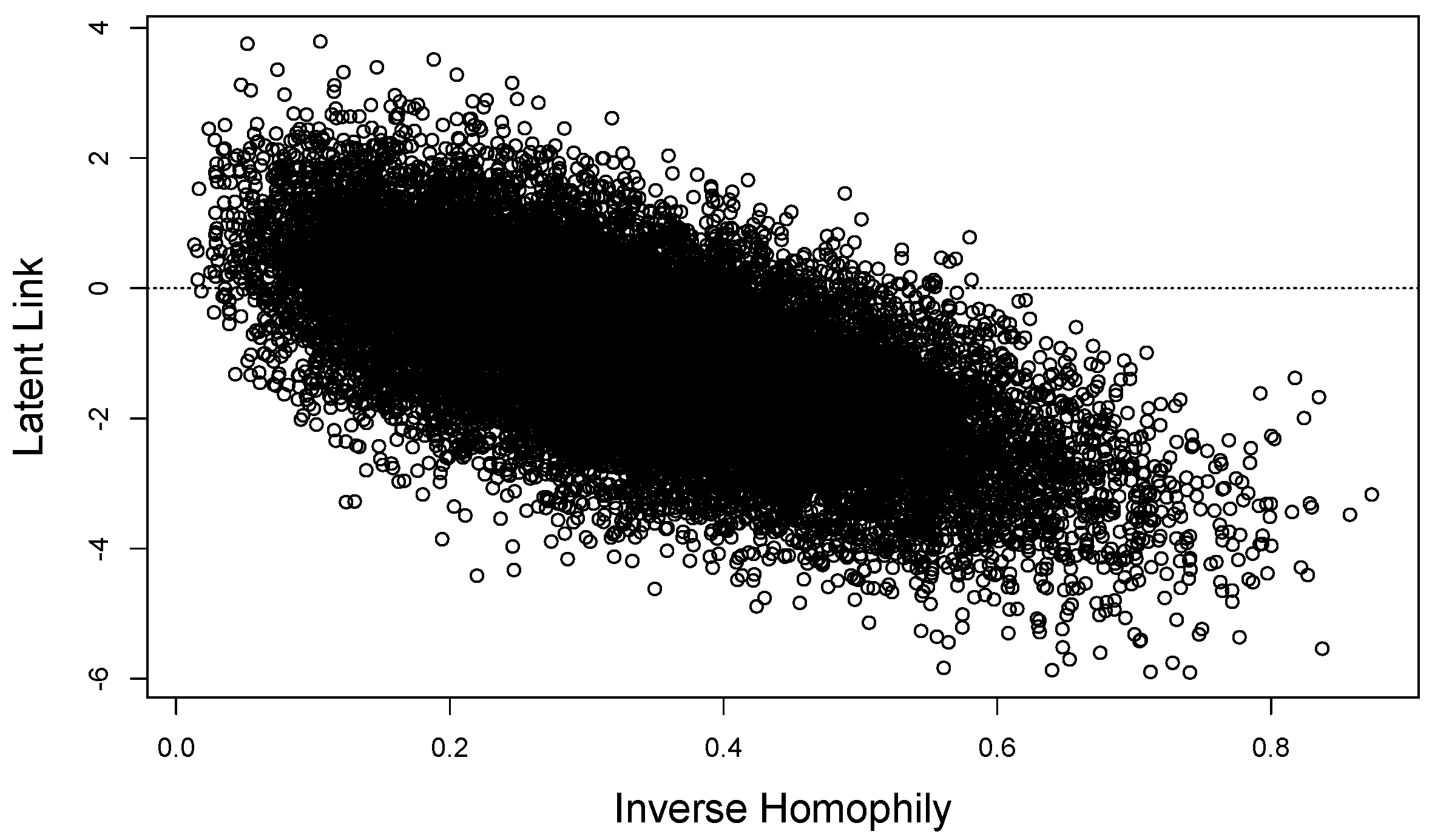
Number of Decision Makers (N)	2000
Number of Global Alternatives (Alternatives in B)	3
Random Terms
Parameters of the Logistic Distribution (mean, scale)	0, 10
Parameters of the Gumbel Distribution (location, scale)	0, 1
Attributes of Each Alternative
SNE model	price, own quality
DNE model	price, own quality, and network quality
Value of True Parameters of the SNE Experiments
Fixed CSF threshold parameter (${\tau }_0$)	0.5
Varying degree of social interaction in CSF	${\tau }_1\in \{0.2,0.4,0.5,0.6,0.8\}$
Fixed utility parameters (ASC1, ASC2, ${\beta }_p$, ${\beta }_{\mathrm{OWN}}$, ${\beta }_{\mathrm{NET}}$) ${}^{\mathrm{a}}$	2, 1, −3, 5, 0
Value of True Parameters of the DNE Experiments
Fixed CSF threshold parameter (${\tau }_0$)	0.5
Varying degree of social interaction in CSF	${\tau }_1\in \{0.2,0.4,0.5,0.6,0.8\}$
Fixed utility parameters (ASC1, ASC2, ${\beta }_p$, β) ${}^{\mathrm{b}}$	2, 1, −3, 5
Varying degree of social interaction in choice	${\alpha }_1\in \{0.2,0.5,0.8\}$ c
Number of Replications (datasets within an experiment)	400

${}^{\mathrm{a}.}$ ASC1 and ASC2 are alternative specific constants for Alternative 1 and Alternative 2, respectively (Alternative 3 is the baseline). They represent normalized utility not captured by price and quality attributes. These parameters reflect average utility differences relative to Alternative 3; ${}^{\mathrm{b}.}$ The parameter $\beta ={\beta }_{\mathrm{OWN}}+{\beta }_{\mathrm{NET}}$ represents the combined effect of own and network quality, refer to Equation (11); ${}^{\mathrm{c}.}$ The experiments implement varying degrees of social interaction in choice by using different pairs of ${\beta }_{\mathrm{OWN}}$ and ${\beta }_{\mathrm{NET}}$ such that ${\beta }_{\mathrm{OWN}}+{\beta }_{\mathrm{NET}}=5$. Specifically we use: {${\beta }_{\mathrm{OWN}}=4,{\beta }_{\mathrm{NET}}=1$} for ${\alpha }_1=0.2$, {${\beta }_{\mathrm{OWN}}=2.5,{\beta }_{\mathrm{NET}}=2.5$} for ${\alpha }_1=0.5$, and {${\beta }_{\mathrm{OWN}}=1,{\beta }_{\mathrm{NET}}=4$} for ${\alpha }_1=0.8$.

. We perform two sets of experiments. The first set consists of 5 experiments with DGP following the SNE model. These experiments vary the degree of social of social interaction in CSF. Specifically, we use ${\tau }_1\in \{0.2,0.4,0.5,0.6,0.8\}$. The second set consists of 15 experiments in which the DGP is determined by the DNE model. These experiments vary both the degree of social interaction in CSF and the degree of social interaction in choice. Specifically, we use ${\tau }_1\in \{0.2,0.4,0.5,0.6,0.8\}$ and ${\alpha }_1\in \{0.2,0.5,0.8\}$. The DNE experiments implement varying degrees of social interaction in choice by using different pairs of ${\beta }_{\mathrm{OWN}}$ and ${\beta }_{\mathrm{NET}}$ such that the combined effect ${\beta }_{\mathrm{OWN}}+{\beta }_{\mathrm{NET}}$ is equal to the effect of own quality in the SNE. This design makes the the total effect of quality on utility comparable between SNE and DNE experiments, which is important when evaluating welfare estimates.

Each experiment considers a population of 2000 decision makers and 3 alternatives in a global choice set. These alternatives differ in price and quality. For each alternative, price and quality data are drawn (independently) from a uniform distribution U(0, 1) to construct ($2000\times 3$) matrix that collects $p_{nj}$ and $q_{nj}$, for $n=1,...,2000$ and $j=1,2,3$.10 This set of price and quality data are utilized in all replications of all experiments.

To generate the social network matrix W, we split our population of 2000 decision makers into 10 groups of 200 individuals representing 10 social networks. This structure mimics a situation in which the econometrician has access to network data on distinct social groups and builds a block diagonal matrix W in which each block corresponds to a social network, e.g., a school, groups of coworkers in companies offices, or a neighborhood.

We use a dyadic regression model to generate links between two individuals in a social network. To mimic real-world social networks, our model incorporates homophily, i.e., the tendency of similar individuals to be connected with each other. This feature is typically observed in social network data (Smith et al. [46]; Leszczensky and Pink [47]). We measure homophily of dyads based on quality perceptions. Our measure is constructed as follows. For each alternative $j\in \{1,2,3\}$, we compute the root square difference between quality perceptions of individuals n and m as:

$$RS{D}_{n,m,j}=\sqrt{{(q_{j,n}-q_{j,m})}^2}.$$

Next, for each dyad $n,m$, we construct the inverse homophily index $H_{n,m}$ as the average of the root square difference across alternatives:

$$H_{n,m}=\frac{1}{3}\sum _{j=1}^{3}RS{D}_{n,m,j}.$$

To construct matrix A (see Section 3.1), we develop a latent variable model in which a link is observed ($Y_{n,m}=1$) if latent link $Y_{n,m}^{*}\ge 0$:

$${\mathrm{Y}}_{n,m}=1\{{\delta }_0-{\delta }_1{H}_{n,m}+{\zeta }_{n,m}\ge 0\}$$

(16)

where ζ is a standard normal error, ${\delta }_0=1$, and ${\delta }_1=6$. To provide an illustration of the random network formation model, Figure 1 and Figure 2 show the generated data for the first block of A. Figure 1 shows the scatter plot of latent link ($Y_{n,m}^{*}$) and inverse homophily ($H_{n,m}$), making it evident that decision makers with similar quality perceptions are more likely to be connected in the social network. Figure 2 shows the histogram of ($Y_{n,m}^{*}$). Dyads above the dashed line in Figure 1, or in the shaded are to the right of the dashed line in Figure 2, are socially connected and corresponds to a network density of 0.22.11 Once A is generated, it is straightforward to compute W and calculate network quality $\tilde{q}$.

Each experiment creates 400 datasets (or replications). In each replication first stage (CSF) errors ${\xi }_{nj}$ are (independently) drawn from a logistic distribution with mean zero and scale $\mu =10$. Following Equation (9), alternatives that satisfy the criteria $\left((1-{\tau }_1)q_{nj}+{\tau }_1{\tilde{q}}_{nj}>{\tau }_0+{\xi }_{nj}\right)$ are included in decision maker n’s choice set, where ${\tau }_0=0.5$ in all experiments.12 In the second stage, decision makers compare utilities of the alternatives available in their choice sets (and determined by the CSF process described above). The alternative that offers the highest utility is chosen. Recall that utility has two components, systematic utility V plus a random component ε. We draw ${\epsilon }_n$ from a Gumbel distribution G(0,1). For simplicity, we assume that V takes a linear functional form $V=x^{\prime }\beta$, where x is a vector of alternative attributes. In the SNE model, attributes are alternative-specific constants, price, and own quality. Network quality is added as an attribute in the DNE model (see Table 1).

In each replication of the SNE experiments we use the simulated data to estimate two sets of parameters. The first, ${\widehat{\theta }}_{SNE}=({\widehat{\beta }}_{\mathrm{OWN}},{\widehat{\tau }}_0,{\widehat{\tau }}_1,\widehat{\mu })$ is obtained through ML estimation of our network SNE model. The second, ${\widehat{\theta }}_{IAL,S}=({\widehat{\beta }}_{\mathrm{OWN}},{\widehat{\tau }}_0,\widehat{\mu })$ is obtained from ML estimation of the standard IAL model. Similarly, in each replication of the DNE experiments we estimate ${\widehat{\theta }}_{DNE}=({\widehat{\beta }}_{\mathrm{OWN}},{\widehat{\beta }}_{\mathrm{NET}},{\widehat{\tau }}_0,{\widehat{\tau }}_1,\widehat{\mu })$ and parameters of the IAL model ${\widehat{\theta }}_{IAL,D}=({\widehat{\beta }}_{\mathrm{OWN}},{\widehat{\tau }}_0,\widehat{\mu })$. Note that estimates ${\widehat{\theta }}_{IAL,S}$ and ${\widehat{\theta }}_{IAL,D}$ are obtained using the same estimator, however they differ because estimation uses different data.

5.1. Evaluating Parameter Estimates

We evaluate our estimates $\widehat{\theta }$ by measuring their average differences to the true set of parameters θ. To facilitate interpretation, we compute errors as a proportion of the magnitude of the parameters. Specifically, we compute the proportional Root Mean Squared Error (RMSE) as follows:

$$\mathrm{Proportional}{\mathrm{RMSE}}_{\theta }=\frac{1}{R}\sum _{r=1}^R\sqrt{{\left(\frac{{\widehat{\theta }}_r-\theta }{\theta }\right)}^2},$$

(17)

where $r=1,...,R$ indexes replications, $R=400$ is the number of replications in each experiment, and $\widehat{\theta }$ represents an estimate of θ. The proportional RMSE directly measures (an average) percentage deviation of estimates from the true parameter values and can be thought of as a coefficient of variation for the experiment.

The expected value of estimates is calculated by the average of parameter estimates of each experiment:

$$E[\widehat{\theta }]=\frac{1}{R}\sum _{r=1}^R{\widehat{\theta }}_r,$$

(18)

Note that comparison between θ and $E[\widehat{\theta }]$ provides an indication of bias whereas the proportional RMSE accounts for the dispersion of the empirical distribution of $\widehat{\theta }$ (obtained form the experiment).

5.2. Evaluating Welfare Estimates

We consider a hypothetical project to investigate how the effect of ignoring social networks on estimates of welfare change. To simulate a project, we consider a 0.4 quality improvement on Alternative 2, i.e., $q_{n2}^1=q_{n2}^0+0.4$, for all n. Following the same logic of previous simulations, we obtain estimates of welfare based on estimates of the SNE, DNE, and IAL models. These welfare estimates are computed by substituting the corresponding vector $\widehat{\theta }$ into expression (15). We evaluate each experiment by reporting an average $\widehat{CV}$ for the entire experiment (i.e., an average across the 2000 decision makers and 400 replications).

We also use the proportional RMSE to evaluate the effect of ignoring social networks (when they are part of the DGP) on welfare estimates. Clearly, the true welfare change is needed to compute such an error. As we observe the draws of the error terms we are able to calculate the true welfare measure ($CV$). It is simply the difference of random utilities of the alternatives that have been chosen before and after the policy change. Specifically, the true $CV$ for individual n in replication r is calculated as

$$\begin{array}{cc}\hfill C{V}_{true,n,r}& =\frac{U_{chosen,n,r}^1-U_{chosen,n,r}^0}{{\beta }_y}\hfill \\ & =\frac{({\mathbf{x}}_{chosen,n,r}^1\beta +{\epsilon }_{chosen,n,r}^1)-({\mathbf{x}}_{chosen,n,r}^0\beta +{\epsilon }_{chosen,n,r}^0)}{{\beta }_y},\hfill \end{array}$$

(19)

where 0 and 1 represent the states of the world before and after the quality improvement (respectively) and ${\beta }_y=-{\beta }_{price}$.13 Matching the unit of analysis of $\widehat{CV}$, we compute an average of true welfare by averaging $CV$ for the entire experiment (i.e., an average of the 2000 decision makers in all 400 replications).

The proportional RMSE considers the variations within an experiment and is calculated as follows:

$$\mathrm{Proportional}\mathrm{RMSE}{}_{CV}=\frac{1}{R}\sum _{r=1}^R\sqrt{{\left(\frac{\widehat{C{V}_r}-C{V}_r}{C{V}_r}\right)}^2},$$

(20)

where $\widehat{C{V}_r}$ is average (over the number of decision makers) estimated $CV$ in replication r, and $C{V}_r$ is the corresponding average true mean $CV$. Notice that the welfare is a dollar measure and the proportional RMSE is a percentage.

6. Results

6.1. SNE Experimets

6.1.1. SNE Parameter Estimates

Table 2. SNE DGP—Mean parameter estimates.

SNE:	${\mathit{\tau }}_1$
	0.2	0.4	0.5	0.6	0.8
ASC1 {2}	2.0068 (0.0512)	2.0046 (0.0453)	2.0057 (0.0438)	1.9988 (0.0470)	1.9892 (0.0397)
ASC2 {1}	0.9986 (0.0580)	0.9956 (0.0547)	1.0029 (0.0495)	1.0061 (0.0432)	1.0012 (0.0387)
Price {−3}	−3.0217 (0.0573)	−3.0112 (0.0553)	−2.9991 (0.0523)	−3.0182 (0.0483)	−3.0135 (0.0427)
Quality {5}	5.0148 (0.0583)	5.0115 (0.0630)	4.9913 (0.0579)	5.0081 (0.0478)	5.0521 (0.0431)
${\tau }_0$ {0.5}	0.5003 (0.0380)	0.4999 (0.0410)	0.5000 (0.0390)	0.5001 (0.0365)	0.5011 (0.0370)
${\tau }_1$ {varied}	0.1988 (0.0206)	0.4023 (0.0363)	0.4992 (0.0413)	0.5994 (0.0401)	0.8052 (0.0404)
μ {10}	10.0404 (0.0425)	10.0680 (0.0426)	10.0199 (0.0426)	10.0279 (0.0390)	10.0270 (0.0416)
IAL:	${\mathbf{\tau }}_{\mathbf{1}}$
	0.2	0.4	0.5	0.6	0.8
ASC1 {2}	2.0001 (0.0599)	1.9671 (0.0653)	1.9051 (0.0817)	1.8170 (0.1146)	1.6460 (0.2157)
ASC2 {1}	0.9917 (0.0751)	0.9590 (0.0908)	0.9310 (0.1118)	0.8798 (0.1436)	0.7718 (0.2671)
Price {−3}	−3.0289 (0.0704)	−2.9707 (0.0867)	−2.8956 (0.0974)	−2.7878 (0.1153)	−2.6186 (0.1992)
Quality {5}	4.9830 (0.0710)	4.9823 (0.0856)	4.9689 (0.0857)	4.9383 (0.0980)	4.8769 (0.1361)
${\tau }_0$ {0.5}	0.5025 (0.0430)	0.5000 (0.0522)	0.4953 (0.0569)	0.4847 (0.0643)	0.4525 (0.1517)
μ {10}	8.9504 (0.1057)	7.7838 (0.2216)	7.2074 (0.2793)	6.6611 (0.3339)	5.3400 (0.4660)

Proportional RMSEs are in parentheses. True parameter values are in curly brackets.

presents the mean estimates ${\widehat{\theta }}_{SNE}$ and ${\widehat{\theta }}_{IAL}$ of the SNE experiments. The columns of the table correspond to different experiments that vary the degree of social interaction in CSF, i.e., ${\tau }_1$. The upper panel reports SNE estimates, i.e., ML estimates obtained from the correctly specified likelihood function. The lower panel reports standard IAL estimates that ignore the social network effects in the CSF process.

Not surprisingly, in all experiments the mean estimates of the correctly specified network model, $E[{\widehat{\theta }}_{SNE}]$, are very similar to the true parameter values θ. For instance, the first column of Table 2 (upper panel) shows that, in the experiment with ${\tau }_1=0.2$, the mean SNE estimate of the price coefficient is $-3.0217$, i.e., a value close to the coefficient’s true value of $-3$. Standard IAL mean estimates, $E[{\widehat{\theta }}_{IAL}]$, tend to underestimate the absolute value of true parameters. While biases are relatively small for ${\tau }_1=0.2$, they are large for higher degrees of social interactions in CSF. Specifically, all IAL estimates monotonically decrease (in absolute value) as the true value of ${\tau }_1$ increases. For instance, the lower panel of Table 2 shows that the mean estimate of quality is equal to 4.9830 for ${\tau }_1=0.2$ and decreases to 4.8769 when ${\tau }_1=0.8$. The results suggest that failure to capture social network effects in CSF may only slightly bias the estimates of IAL parameters when the degree of social interaction in CSF of the underlying data generating process is low. On the other hand, our simulations show significant biases for higher levels of ${\tau }_1$.

The efficiency of estimation is evaluated through the proportional RMSEs. These errors are presented in parenthesis below the corresponding $E[\widehat{\theta }]$ estimate in Table 2. For the most part, proportional RMSEs of the SNE estimates are below 5%. In general, errors of the utility parameters decrease with the degree of social interaction in CSF. Errors of the CSF parameters tend to be smaller than those of the utility parameters and fluctuate below 5% in all experiments.

The proportional RMSEs of IAL estimates are above 5%,14 and are always larger than the corresponding SNE error estimate. The errors increases (monotonically) as the degree of social interaction in CSF increases from ${\tau }_1=0.2$ to ${\tau }_1=0.8$, and are very large when social interaction is high. For instance, the IAL mean errors of price and quality for ${\tau }_1=0.8$ are 19.9% and 13.6% of true parameter values, respectively. In summary, our simulation results indicate that ignoring social network effects on IAL CSF processes can significantly increase both the bias and the variance of IAL estimates, especially when the degree of social interaction in CSF is high.

6.1.2. SNE Market Shares

Let us now examine the distribution of choices made by individuals in the second stage of our models. These choices determine the market shares of each alternative. We compute an experiment-level measure of alternative j’s market share by averaging the proportion of individuals that chooses j over the 400 replications. We calculate market shares predicted by the SNE and IAL models and true market shares.

Contrary to choice sets, that are unknown to the econometrician, market shares are known as they are based on observed choices.15 The econometrician, however, may be interested in forecasting market shares, for example, to estimate the changes in market shares induced by a project that modifies attributes of alternatives (e.g., an increase in the quality of alternative 2). In a “no Lucas critique” scenario, the econometrician can predict market shares before and after the implementation of a hypothetical project by using available estimates $\widehat{\theta }$ paired with pre-project data and information on how the project modifies attributes (i.e., hypothetical post-project data).16

Table 3. SNE DGP—Market shares of True, SNE, and IAL models, before and after the policy, and market share change.

(${\mathit{\tau }}_1$ = 0.2)
Consumer Choice	Before			After			Change
	True	SNE	IAL	True	SNE	IAL	True	SNE	IAL
{1}	0.407	0.407 (0.015)	0.407 (0.014)	0.245	0.245 (0.032)	0.251 (0.036)	−0.163	−0.162 (0.022)	−0.157 (0.044)
{2}	0.327	0.326 (0.013)	0.327 (0.015)	0.644	0.643 (0.014)	0.630 (0.023)	0.317	0.317 (0.017)	0.304 (0.044)
{3}	0.266	0.266 (0.020)	0.266 (0.018)	0.111	0.112 (0.031)	0.119 (0.075)	−0.155	−0.155 (0.019)	−0.147 (0.050)
(${\mathbf{\tau }}_{\mathbf{1}}$ = 0.8)
Consumer Choice	Before			After			Change
	True	SNE	IAL	True	SNE	IAL	True	SNE	IAL
{1}	0.402	0.401 (0.020)	0.403 (0.020)	0.224	0.221 (0.045)	0.248 (0.114)	−0.179	−0.179 (0.018)	−0.154 (0.137)
{2}	0.325	0.325 (0.012)	0.324 (0.022)	0.678	0.681 (0.016)	0.615 (0.093)	0.353	0.355 (0.024)	0.291 (0.177)
{3}	0.273	0.274 (0.024)	0.273 (0.026)	0.098	0.098 (0.021)	0.136 (0.393)	−0.175	−0.176 (0.038)	−0.137 (0.218)

Proportional RMSEs are in parentheses.

shows true and predicted market shares of each alternative before the project, after the project, and the change in market shares induced by the project. For the experiment with low degree of social interaction in CSF (${\tau }_1=0.2$), the upper panel of the table shows that the project increases the market share of alternative 2 from 0.327 to 0.644, i.e., an increase of 0.317. The SNE model performs very well in predicting this increase in market share: the SNE prediction shows no bias and a proportional RMSE of 0.017. In contrast, the IAL underestimates the market share gain by 4% (0.304 to 0.317) with a mean error of approximately 4.4%. Confirming the tendency being established by the paper, the performance of the IAL estimates deteriorate in experiments with high degree of social interaction. For example, in the experiment with ${\tau }_1=0.8$ (lower panel of Table 3), while the SNE slightly overestimates the market share gain of alternative 2, the IAL underestimates the market gain by 17.6% (0.291 to 0.353). As a result, failure to account for network effects in CSF when predicting the impact of projects may lead managers to incorrectly not put forward beneficial projects.

6.1.3. SNE Welfare Estimates

Table 4. SNE DGP—Mean welfare of True, SNE and IAL models.

Models	${\mathit{\tau }}_1$
	0.2	0.4	0.5	0.6	0.8
True	0.3784	0.3895	0.3956	0.4025	0.4181
SNE	0.3728 (0.0814)	0.3814 (0.0843)	0.3865 (0.0842)	0.3906 (0.0747)	0.4076 (0.0737)
IAL	0.3649 (0.0984)	0.3721 (0.1113)	0.3822 (0.1166)	0.3950 (0.1311)	0.4254 (0.2066)

Proportional RMSEs are in parentheses.

presents the average ${\widehat{CV}}_{SNE}$ (SNE welfare estimate), ${\widehat{CV}}_{IAL}$ (IAL welfare estimate), and $CV$ (true welfare measure) for all SNE experiments. The SNE estimates of the mean compensating variation are similar to the true mean $CV$. The average ${\widehat{CV}}_{SNE}$ slightly underestimates the average $CV$. Interestingly, while the differences between mean ${\widehat{CV}}_{SNE}$ and mean $CV$ slightly increase with ${\tau }_1$, the dispersion of ${\widehat{CV}}_{SNE}$ generally decreases with ${\tau }_1$. This behavior was also observed in Table 2 (upper panel) that reports the proportional RMSEs of utility parameter estimates of the SNE model.

The IAL model underestimates true mean $CV$ by 3.6%, 4.5%, and 3.4% when ${\tau }_1$ is equal to 0.2, 0.4, and 0.5, respectively. For ${\tau }_1\ge 0.6$, the IAL welfare estimates present little bias. In this range, the difference between ${\widehat{CV}}_{IAL}$ and $CV$ is smaller than that between ${\widehat{CV}}_{SNE}$ and $CV$. While the biases of IAL estimates of welfare are relatively small, especially at high ranges of ${\tau }_1$, the variance of these estimates monotonically increases with the degree of social interaction in CSF. Proportional RMSEs increase from approximately 10% when ${\tau }_1=0.2$ and reach 21% when ${\tau }_1=0.8$. This behavior also follows the pattern of mean errors of parameter estimates (see proportional RMSEs of IAL parameter estimates in Table 2).

6.2. DNE Experimets

6.2.1. DNE Parameter Estimates

This section reports results of parameter estimates of the DNE experiments. Recall that the DNE DGP is equal to that of the SNE experiments, except that individual n’s random utility from alternative j is equal to:

$$U_{nj}=AS{C}_j+{\beta }_p{p}_{nj}+{\beta }_{\mathrm{OWN}}{q}_{nj}+{\beta }_{\mathrm{NET}}{\tilde{q}}_{nj}+{\epsilon }_{nj}.$$

Table 5. DNE DGP—Mean DNE estimates of the degree of social interaction in choice set formation (CSF) (${\tau }_1$), the degree of social interaction in choice (${\alpha }_1$), and the combined quality effect (β).

Estimates of ${\mathit{\tau }}_1$	${\mathit{\tau }}_1$
${\mathit{\alpha }}_{\mathbf{1}}$	0.2	0.4	0.5	0.6	0.8
0.2	0.2001 (0.0130)	0.4011 (0.0308)	0.5005 (0.0408)	0.5974 (0.0411)	0.8018 (0.0393)
0.5	0.2015 (0.0178)	0.4015 (0.0327)	0.5002 (0.0376)	0.5980 (0.0401)	0.8008 (0.0363)
0.8	0.1996 (0.0137)	0.4029 (0.0309)	0.4999 (0.0321)	0.5990 (0.0359)	0.8021 (0.0355)
Estimates of ${\mathit{\alpha }}_{\mathbf{1}}$	${\mathit{\tau }}_{\mathbf{1}}$
${\mathit{\alpha }}_{\mathbf{1}}$	0.2	0.4	0.5	0.6	0.8
0.2	0.1998 (0.0395)	0.2014 (0.0376)	0.2007 (0.0401)	0.2020 (0.0383)	0.2012 (0.0318)
0.5	0.5002 (0.0163)	0.4997 (0.0144)	0.4995 (0.0190)	0.5001 (0.0153)	0.5008 (0.0108)
0.8	0.7978 (0.0063)	0.7989 (0.0067)	0.7992 (0.0055)	0.7992 (0.0036)	0.7997 (0.0025)
Estimates of β	${\mathit{\tau }}_{\mathbf{1}}$
${\mathit{\alpha }}_{\mathbf{1}}$	0.2	0.4	0.5	0.6	0.8
0.2	5.0327 (0.0450)	4.9930 (0.0388)	5.0208 (0.0447)	4.9847 (0.0449)	4.9955 (0.0349)
0.5	5.0119 (0.0309)	5.0151 (0.0246)	5.0017 (0.0257)	4.9734 (0.0227)	5.0177 (0.0216)
0.8	4.9980 (0.0293)	5.0397 (0.0290)	4.9807 (0.0271)	4.9858 (0.0245)	5.0016 (0.0168)

Proportional RMSEs are in parentheses.

focuses on DNE estimates of first stage and second stage network parameters; degree of social interaction in CSF ${\tau }_1$, degree of social interaction in choice ${\alpha }_1={\beta }_{\mathrm{NET}}/({\beta }_{\mathrm{OWN}}+{\beta }_{\mathrm{NET}})$, and combined quality effect $\beta ={\beta }_{\mathrm{OWN}}+{\beta }_{\mathrm{NET}}$. The table compiles $E[{\widehat{\theta }}_{DNE}]$ of 15 experiments corresponding to 15 DGPs that follow the DNE model using $\beta =5$ and all combinations of ${\tau }_1\in \{0.2,0.4,0.5,0.6,0.8\}$ and ${\alpha }_1\in \{0.2,0.5,0.8\}$. For each experiment, and in each replication, an estimate ${\alpha }_1$ is obtained as ${\widehat{\beta }}_{\mathrm{NET}}/({\widehat{\beta }}_{\mathrm{OWN}}+{\widehat{\beta }}_{\mathrm{NET}})$ and $E[{\widehat{\alpha }}_1]$ is the average ${\widehat{\alpha }}_1$ across the 400 replications. A similar procedure is used to obtain $E[\widehat{\beta }]$. The table also reports proportional RMSEs of these DNE estimates.

In all experiments, the expected values of the all three parameters are very close to their respective true values. All parameters are estimated with proportional RMSEs below 5%. Interestingly, the estimation of the utility parameters ${\alpha }_1$ and β becomes even more efficient when the degree of social interaction in choice ${\alpha }_1$ increases. For example, the middle panel of Table 5 shows that the proportional RMSE of ${\widehat{\alpha }}_1$ in experiment $({\tau }_1=0.8,{\alpha }_1=0.2)$ is 0.0318 and it decreases to 0.0025 in experiment $({\tau }_1=0.8,{\alpha }_1=0.8)$.

The first two panels of

Table 6. DNE DGP—Mean estimates of price, own quality, and network quality parameters.

Price Parameter Estimates
{${\mathit{\beta }}_{\mathrm{OWN}}$, ${\mathit{\beta }}_{\mathrm{NET}}$}	Models	${\mathit{\tau }}_{\mathbf{1}}$
		0.2	0.4	0.5	0.6	0.8
{4, 1}	DNE	−2.9827 (0.0495)	−3.0090 (0.0507)	−2.9933 (0.0475)	−3.0005 (0.0449)	−2.9981 (0.0471)
	IAL	−3.0054 (0.0659)	−2.9831 (0.0842)	−2.8890 (0.1009)	−2.7934 (0.1258)	−2.7541 (0.1909)
{2.5, 2.5}	DNE	−2.9979 (0.0480)	−3.0108 (0.0476)	−2.9912 (0.0432)	−3.0163 (0.0421)	−3.0011 (0.0357)
	IAL	−3.0791 (0.0771)	−3.0421 (0.0826)	−2.9807 (0.1032)	−2.9439 (0.1287)	−2.8302 (0.1613)
{1, 4}	DNE	−3.0064 (0.0488)	−2.9968 (0.0473)	−2.9926 (0.0416)	−3.0041 (0.0413)	−3.0035 (0.0334)
	IAL	−3.2701 (0.1088)	−3.1576 (0.0815)	−3.1677 (0.1062)	−3.1762 (0.1330)	−3.5588 (0.2295)
Own Quality Parameter Estimates
{${\mathit{\beta }}_{\mathbf{OWN}}$, ${\mathit{\beta }}_{\mathbf{NET}}$}	Models	${\mathit{\tau }}_{\mathbf{1}}$
		0.2	0.4	0.5	0.6	0.8
{4, 1}	DNE	4.0323 (0.0550)	3.9928 (0.0493)	4.0200 (0.0544)	3.9845 (0.0474)	3.9949 (0.0425)
	IAL	4.2493 (0.0903)	4.3142 (0.1117)	4.3561 (0.1244)	4.3446 (0.1307)	4.2888 (0.1635)
{2.5, 2.5}	DNE	2.5074 (0.0408)	2.5119 (0.0362)	2.4995 (0.0346)	2.4900 (0.0356)	2.5068 (0.0300)
	IAL	3.0340 (0.2148)	3.1055 (0.2445)	3.3559 (0.3465)	3.4283 (0.3818)	3.4482 (0.3896)
{1, 4}	DNE	1.0045 (0.0192)	1.0074 (0.0202)	0.9949 (0.0189)	0.9982 (0.0154)	1.0000 (0.0103)
	IAL	1.3030 (0.3030)	1.2917 (0.2917)	1.5384 (0.5385)	1.9042 (0.9050)	2.1963 (1.2043)
Network Quality Parameter Estimates
{${\mathit{\beta }}_{\mathbf{OWN}}$, ${\mathit{\beta }}_{\mathbf{NET}}$}	Models	${\mathit{\tau }}_{\mathbf{1}}$
		0.2	0.4	0.5	0.6	0.8
{4, 1}		1.0004 (0.0075)	1.0002 (0.0075)	1.0008 (0.0076)	1.0002 (0.0058)	1.0007 (0.0055)
{2.5, 2.5}	DNE	2.5044 (0.0261)	2.5032 (0.0184)	2.5023 (0.0220)	2.4834 (0.0177)	2.5109 (0.0164)
{1, 4}		3.9935 (0.0342)	4.0323 (0.0348)	3.9858 (0.0303)	3.9876 (0.0272)	4.0017 (0.0187)

Proportional RMSEs are in parentheses.

report the expected values of DNE and IAL estimates of the parameters of price (${\beta }_p$) and own quality (${\beta }_{\mathrm{OWN}}$). The bottom panel reports DNE average estimates of the network quality parameter (${\beta }_{\mathrm{NET}}$).17 The table shows that the expected value of the DNE estimates is very close to true parameter values. The proportional RMSEs are generally below 5% indicating the distributions of DNE estimates are quite narrow around true parameter values, especially for the network quality parameter ${\beta }_{\mathrm{NET}}$.

The expected value of IAL estimates of the price parameter is generally smaller (in absolute value) than the true negative effect (−3) in the experiments with ${\alpha }_1=0.2$ and ${\alpha }_1=0.5$.18 This bias gets stronger with higher degrees of social interaction in CSF ${\tau }_1$. For high levels of social interaction in choice (the experiments with ${\alpha }_1=0.8$), the IAL overestimates the price effects, especially in experiments with extreme values of social interaction in CSF, ${\tau }_1=0.2$ and ${\tau }_1=0.8$. In general, both bias and variance of the IAL estimates increase as we move from the north-west corner to the south-east corner of the IAL panels in Table 6. In all experiments, the IAL overestimates the parameter of own quality ${\beta }_{\mathrm{OWN}}$, however, never to the point that ${\beta }_{\mathrm{OWN}}$ captures the true combined quality effect $\beta =5$. In other words, we find that ${\beta }_{\mathrm{OWN}}<E[{\widehat{\beta }}_{\mathrm{OWN}}^{\mathrm{IAL}}]<\beta$. As with price estimates, own quality estimates deteriorate with increases in both ${\tau }_1$ and ${\alpha }_1$.

6.2.2. DNE Market Shares

Table 7. DNE DGP—Market shares of True, DNE, and IAL models, before and after the policy, and market share change.

(${\mathit{\beta }}_{\mathbf{OWN}}$ = 4, ${\mathit{\beta }}_{\mathbf{NET}}$ = 1, ${\mathit{\tau }}_1$ = 0.2)
Consumer Choice	Before			After			Change
	True	DNE	IAL	True	DNE	IAL	True	DNE	IAL
{1}	0.410	0.410 (0.017)	0.409 (0.014)	0.238	0.238 (0.035)	0.259 (0.089)	−0.171	−0.172 (0.021)	−0.150 (0.125)
{2}	0.326	0.327 (0.014)	0.327 (0.016)	0.657	0.659 (0.013)	0.620 (0.057)	0.331	0.332 (0.016)	0.293 (0.115)
{3}	0.264	0.264 (0.022)	0.263 (0.020)	0.104	0.104 (0.034)	0.120 (0.153)	−0.160	−0.160 (0.019)	−0.143 (0.104)
(${\mathit{\beta }}_{\mathbf{OWN}}$ = 4, ${\mathit{\beta }}_{\mathbf{NET}}$ = 1, ${\mathit{\tau }}_{\mathbf{1}}$ = 0.8)
Consumer Choice	Before			After			Change
	True	DNE	IAL	True	DNE	IAL	True	DNE	IAL
{1}	0.405	0.404 (0.020)	0.406 (0.020)	0.217	0.216 (0.046)	0.258 (0.194)	−0.188	−0.188 (0.017)	−0.147 (0.216)
{2}	0.325	0.326 (0.011)	0.324 (0.023)	0.693	0.694 (0.016)	0.604 (0.129)	0.368	0.368 (0.022)	0.280 (0.239)
{3}	0.270	0.271 (0.025)	0.270 (0.025)	0.090	0.090 (0.026)	0.138 (0.524)	−0.180	−0.180 (0.035)	−0.133 (0.263)
(${\mathit{\beta }}_{\mathbf{OWN}}$ = 1, ${\mathit{\beta }}_{\mathbf{NET}}$ = 4, ${\mathit{\tau }}_{\mathbf{1}}$ = 0.2)
Consumer Choice	Before			After			Change
	True	DNE	IAL	True	DNE	IAL	True	DNE	IAL
{1}	0.415	0.415 (0.014)	0.411 (0.017)	0.215	0.216 (0.041)	0.300 (0.395)	−0.200	−0.200 (0.026)	−0.111 (0.447)
{2}	0.325	0.326 (0.013)	0.326 (0.017)	0.699	0.698 (0.015)	0.562 (0.195)	0.373	0.373 (0.017)	0.236 (0.368)
{3}	0.260	0.259 (0.018)	0.263 (0.024)	0.086	0.086 (0.042)	0.137 (0.597)	−0.174	−0.173 (0.016)	−0.125 (0.279)
(${\mathit{\beta }}_{\mathbf{OWN}}$ = 1, ${\mathit{\beta }}_{\mathbf{NET}}$ = 4, ${\mathit{\tau }}_{\mathbf{1}}$ = 0.8)
Consumer Choice	Before			After			Change
	True	DNE	IAL	True	DNE	IAL	True	DNE	IAL
{1}	0.412	0.411 (0.017)	0.411 (0.019)	0.194	0.193 (0.044)	0.296 (0.527)	−0.218	−0.218 (0.014)	−0.115 (0.472)
{2}	0.324	0.325 (0.011)	0.325 (0.020)	0.736	0.737 (0.013)	0.558 (0.242)	0.412	0.412 (0.016)	0.233 (0.433)
{3}	0.264	0.264 (0.020)	0.264 (0.028)	0.070	0.070 (0.030)	0.146 (1.080)	−0.193	−0.194 (0.026)	−0.118 (0.390)

Proportional RMSEs are in parentheses.

presents estimates of market shares before and after the project, and estimates of the predicted changes in the market shares induced by the project.19 The correctly specified DNE model performs remarkably well in all experiments. In general, the DNE predicts the change in the market shares of all alternatives with no bias and proportional RMSEs hover around 0.02. The results also show that IAL estimates are both biased and inefficient, and both the bias and the proportional RMSE increase with the degree of social interaction in CSF and choice. For example, the IAL underestimates the increase of alternative 2’s market share by 23.9% in experiment (${\alpha }_1=0.2,{\tau }_1=0.8$), and by 43.4% in experiment (${\alpha }_1=0.8,{\tau }_1=0.8$). With respect to the variance of the estimates of the change in the market share of alternative 2, the proportional RMSE is 23.9% in experiment (${\alpha }_1=0.2,{\tau }_1=0.8$), and 43.3% in experiment (${\alpha }_1=0.8,{\tau }_1=0.8$). Therefore, the market share estimates corroborate the main lesson from the Monte Carlo experiments and highlights additional issues associated with misspecification of network effects.

6.2.3. DNE Welfare Estimates

Table 8. DNE DGP—Mean welfare of True, DNE, and IAL models.

{${\mathit{\beta }}_{\mathbf{OWN}}$, ${\mathit{\beta }}_{\mathbf{NET}}$}	Models	${\mathit{\tau }}_1$
		0.2	0.4	0.5	0.6	0.8
{4, 1}	True	0.3882	0.3991	0.4015	0.4112	0.4269
	DNE	0.3904 (0.0772)	0.3928 (0.0730)	0.4003 (0.0792)	0.4018 (0.0709)	0.4156 (0.0764)
	IAL	0.3197 (0.1943)	0.3264 (0.1948)	0.3404 (0.1873)	0.3517 (0.1854)	0.3600 (0.2394)
		${\mathit{\tau }}_{\mathbf{1}}$
		0.2	0.4	0.5	0.6	0.8
{2.5, 2.5}	True	0.4040	0.4151	0.4209	0.4268	0.4411
	DNE	0.4056 (0.0663)	0.4124 (0.0609)	0.4177 (0.0634)	0.4167 (0.0614)	0.4336 (0.0599)
	IAL	0.2372 (0.4162)	0.2424 (0.4165)	0.2633 (0.3753)	0.2740 (0.3583)	0.2923 (0.3835)
		${\mathit{\tau }}_{\mathbf{1}}$
		0.2	0.4	0.5	0.6	0.8
{1, 4}	True	0.4224	0.4339	0.4397	0.4452	0.4582
	DNE	0.4245 (0.0637)	0.4382 (0.0609)	0.4373 (0.0576)	0.4411 (0.0606)	0.4515 (0.0496)
	IAL	0.1294 (0.6938)	0.1297 (0.7012)	0.1413 (0.6787)	0.1640 (0.6349)	0.1569 (0.6576)

Proportional RMSEs are in parentheses.

presents true mean welfare and mean welfare estimates of DNE experiments. In all experiments, the DNE estimates of mean compensating variation ${\widehat{CV}}_{DNE}$ are very similar to true $CV$ values. In particular, these estimates present biases of less than 1% when the degree of social interaction in CSF is low, i.e., ${\tau }_1=0.2$. The proportional RMSEs of DNE estimates are significantly smaller than those of the IAL estimates, and the distribution of ${\widehat{CV}}_{DNE}$ becomes narrower as the degree of social interaction in choice increases.

In contrast, the performance of the IAL welfare estimates is extremely poor and ${\widehat{CV}}_{IAL}$ massively underestimates true $CV$. The bias of ${\widehat{CV}}_{IAL}$ increases with the degree of social interaction in choice. This is not surprising as the IAL ignores the effect that social networks add to utility: as this effect gets stronger, the bias increases. The average level of underestimation in the first panel of Table 8 (${\beta }_{\mathrm{OWN}}=4$, ${\beta }_{\mathrm{NET}}=1$) is 16.2%, increases to 38% in the second panel (${\beta }_{\mathrm{OWN}}=2.5$, ${\beta }_{\mathrm{NET}}=2.5$), and reaches 67.3% in the last panel (${\beta }_{\mathrm{OWN}}=1$, ${\beta }_{\mathrm{NET}}=4$). The results also indicate that the distribution of ${\widehat{CV}}_{IAL}$ is very wide. Estimation becomes more inefficient with increases of the underlying level of ${\alpha }_1$ in the DGP. For instance, in the experiment (${\beta }_{\mathrm{OWN}}=4$, ${\beta }_{\mathrm{NET}}=1$, ${\tau }_1=0.2$), the proportional RMSE of ${\widehat{CV}}_{IAL}$ is 0.1943 and increases to 0.6938 in experiment (${\beta }_{\mathrm{OWN}}=1$, ${\beta }_{\mathrm{NET}}=4$, ${\tau }_1=0.2$).

7. Discussion

The economics literature has been evolving rapidly and now offers an array of different types of social interaction discrete choice models (refer to Benhabib et al. [48] for a review). While papers in this literature have examined the effect of advertising on consideration sets (e.g., Sovinsky Goeree [30]; Draganska and Klapper [31]), to the best of our knowledge, our paper is the first to jointly address two fundamental factors of modern decision making processes: choice set formation and the influence of “friends”. This is an important contribution as the modern consumer (e.g., millennials) tends to rely less on advertising and more on peer reviews. However, our examination of this issue has revealed several areas for future research and identified limitations in current approaches.

One area of future research is to evaluate the effect of advertisement accommodating network effects. Take online advertisement for example: Internet companies like Google often have access to information on online social networks, purchases, and exposure to advertising content of different products to different subjects. If quality perceptions are influenced by advertising, one can use advertising information (e.g., type, content, intensity of exposure) to estimate our network models and disentangle advertising operating through own perceptions versus social network perception, in the choice set formation stage against the choice stage.

This paper proposes two discrete choice models: one in which social networks influence solely choice set formation (SNE), and another in which social networks influence the consideration sets and choices (DNE). A natural question is: “which model to employ”? If the research has prior information indicating that social networks influence choice sets but not choice directly (perhaps in a case in which consumers may place most utility weight on their own perceptions of attributes and little weight on the perceptions of friends), then it is only natural to estimate the SNE model. If no prior information is available (which we anticipate would be the most common situation), the researcher should estimate the DNE model that nests the SNE model. We perform Monte Carlo experiments in which the DGP is that of the SNE model and use this data to estimate the DNE parameters. The estimation approach successfully fits ${\beta }_{NET}=0$ predicting the fact that the social network does not influence the choice stage of the model. The model does not show parameter biases and estimation is quite efficient with proportional RMSEs less than 5% (see Supplementary Materials Table S38).

Our paper may also serve as a guide to data collection. Notice that estimation of our models requires only one type of additional information when compared to the data requirements of MNL or IAL models: social network connections. The literature increasingly recognizes that social networks play a role in determining several socio-economic outcomes and scholars are increasingly collecting social network data to examine network interactions in various environments. Examples include research about the diffusion of microfinance (Banerjee et al. [49]), technology adoption (Magnan et al. [50]), trust and informal contracts (Karlan et al. [51]), and food sharing (McMillan and Parlee [52]), to name a few. Other papers have argued that geographical proximity is a significant determinant of interpersonal relationships (Karlan et al. [51]; Fafchamps and Gubert [53]). This opens an avenue for researchers to use Global Positioning System (GPS) data to construct neighbor networks that serve as proxies for social networks (e.g., Ambrus et al. [54]).

The paper has several limitations. First, our model essentially assumes the exogeneity of quality perceptions, which may not be the case if historical choices and experience influence quality perceptions by the individual and his/her network. On one hand this suggests that our approach will be particularly relevant to classes of choices that reflect this condition. This is a large class that includes new goods (where historical choice has no influence), choices where attributes are significantly affected by exogenous variation (for example, weather and natural fluctuations influencing recreation site choice), stated preference experiments (choice experiments) in which attributes are randomly assigned to decision makers, and products that are heavily affected by advertising (that influences product perceptions) since advertising is not expected to be influenced by social networks (friends). In addition, if the bias that may arise from endogeneity is orthogonal to the bias arising from ignoring social networks, then the lessons learned from our experiments hold for a wide class of applications. However, additional research into the presence and impact of endogeneity in a social network setting is an important avenue for future work.

Note that the CSF framework developed by the paper can be adapted to other mechanisms of availability determination. For instance, availability of an alternative may be determined by prices (that are often exogenous), and network effects may also be important. In the context of recreation site choice, parents may form choice sets not only considering own prices but also prices faced by those in their networks like children, other family members, and friends.

Second, as most discrete choice models in the literature, we assume that decision makers form expectations about unknown quantities and make choices to maximize expected utility. As Manski [55] argues, the challenge faced by standard models is that observed choice behavior is often consistent with various preferences and expectations specifications. A new literature shows how self-reported expectation can be incorporated in discrete choice models to relax or validate assumptions about expectations (Manski [55]; van der Klaauw [56]). Future research should investigate interactions between social networks and these subjective probabilities.

Third, our paper (like several others in the literature, e.g., Bramoulle et al. [43]) assumes that the social network is exogenous to other errors in the model; in our case, unobserved determinants of the availability function and utility. Qu and Lee [57] propose estimation methods to address the issue of an endogenous weight matrix. Future work should extend their approaches to a CSF model with social networks. Fourth, we develop a model of CSF and social networks for cases where the econometrician does not observe choice sets (i.e., a probabilistic approach). In a “nonsocial network” context, Draganska and Klapper [31] show how choice set data can be used to estimate discrete choice models. Future work should evolve in this direction and study how choice set information can be incorporated in the estimation of discrete models with social network.

Finally, there is a need to incorporate heterogeneity in choice set formation arising from network influences with search processes that also generate choice sets. Hauser [2] describes a search process that is based on benefit-cost analysis of alternatives, and the use of heuristics. This process helps explain heterogeneity in choice sets and is quite consistent with our approach. To be considered, alternatives must pass a threshold (a benefit-cost like test) that in our case is influenced by friends. If a search process is part of this benefit-cost test then the network also effectively influences awareness and consideration. However, there may be separate roles that search, heuristics, and social influence play in choice set formation and these should be avenues for future research. Moreover, these pathways may vary across product types (e.g., durables versus non-durables, etc.).

References

- J.R. Hauser, O. Toubia, T. Evgeniou, R. Befurt, and D. Dzyabura. “Disjunctions of conjunctions, cognitive simplicity, and consideration sets.” J. Mark. Res. 47 (2010): 485–496. [Google Scholar] [CrossRef]
- J.R. Hauser. “Consideration-set heuristics.” J. Bus. Res. 67 (2014): 1688–1699. [Google Scholar] [CrossRef]
- E. Van Nierop, B. Bronnenberg, R. Paap, M. Wedel, and P.H. Franses. “Retrieving unobserved consideration sets from household panel data.” J. Mark. Res. 47 (2010): 63–74. [Google Scholar] [CrossRef]
- K. Eliaz, and R. Spiegler. “Consideration sets and competitive marketing.” Rev. Econ. Stud. 78 (2011): 235–262. [Google Scholar] [CrossRef] [Green Version]
- J. Swait, and T. Erdem. “Brand effects on choice and choice set formation under uncertainty.” Mark. Sci. 26 (2007): 679–697. [Google Scholar] [CrossRef]
- Forbes. “10 New Findings About The Millennial Consumer.” 2015. Available online: http://www.forbes.com/sites/danschawbel/2015/01/20/10-new-findings-about-the-millennial-consumer/#3528b01828a8 (accessed on 24 June 2016).
- AutoTrader. “The Next Generation Car Buyer: Millennials.” 2013. Available online: http://oemsolutions.agameautotrader.com/wp-content/uploads/2013/05/Millennials-Next-Gen-Car-Buyer.pdf (accessed on 24 June 2016).
- Automotive News. “BMW Tailors its Pitch to the Young and Wealthy.” 2016. Available online: http://www.autonews.com/article/20160113/OEM09/160119822/bmw-tailors-its-pitch-to-the-young-and-wealthy (accessed on 24 June 2016).
- W. Zavoina, and R.D. McKelvey. “A statistical model for the analysis of ordinal level dependent variables.” J. Math. Sociol. 4 (1975): 103–120. [Google Scholar]
- D. McFadden. “Conditional Logit Analysis of Qualitative Choice Behavior.” In Frontiers in Econometrics. Edited by P. Zarembka. London, UK: New York, NY, USA: Academic Press, 1974, pp. 105–142. [Google Scholar]
- J. Swait, and M. Ben-Akiva. “Incorporating random constraints in discrete models of choice set generation.” Transp. Res. B Methodol. 22 (1987): 91–102. [Google Scholar] [CrossRef]
- L. Li, W.L. Adamowicz, and J. Swait. “The effect of choice set misspecification on welfare measures in random utility models.” Resour. Energy Econ. 42 (2015): 71–92. [Google Scholar] [CrossRef]
- M. Bierlaire, R. Hurtubia, and G. Flötteröd. “Analysis of implicit choice set generation using a constrained multinomial logit model.” Transp. Res. Rec. 2175 (2010): 92–97. [Google Scholar] [CrossRef]
- J. Andreoni. “Impure altruism and donations to public goods: A theory of warm-glow giving.” Econ. J. 100 (1990): 464–477. [Google Scholar] [CrossRef]
- M. Rabin. “Incorporating fairness into game theory and economics.” Am. Econ. Rev. 5 (1993): 1281–1302. [Google Scholar]
- S.D. Levitt, and J.A. List. “What do laboratory experiments measuring social preferences reveal about the real world? ” J. Econ. Perspect. 21 (2007): 153–174. [Google Scholar] [CrossRef]
- W. Neilson, and B. Wichmann. “Social networks and non-market valuations.” J. Environ. Econ. Manag. 67 (2014): 155–170. [Google Scholar] [CrossRef]
- E. Duflo, and E. Saez. “Participation and investment decisions in a retirement plan: The influence of colleagues choices.” J. Public Econ. 85 (2002): 121–148. [Google Scholar] [CrossRef]
- S.M. Chowdhury, and J.Y. Jeon. “Impure altruism or inequality aversion?: An experimental investigation based on income effects.” J. Public Econ. 118 (2014): 143–150. [Google Scholar] [CrossRef]
- W.A. Brock, and S.N. Durlauf. “Discrete choice with social interactions.” Rev. Econ. Stud. 68 (2001): 235–260. [Google Scholar] [CrossRef]
- L.-F. Lee, J. Li, and X. Lin. “Binary choice models with social network under heterogeneous rational expectations.” Rev. Econ. Stat. 96 (2014): 402–417. [Google Scholar] [CrossRef]
- A.R. Soetevent, and P. Kooreman. “A discrete-choice model with social interactions: With an application to high school teen behavior.” J. Appl. Econ. 22 (2007): 599–624. [Google Scholar] [CrossRef]
- T.J. Richards, S.F. Hamilton, and W.J. Allender. “Social networks and new product choice.” Am. J. Agric. Econ. 96 (2014): 489–516. [Google Scholar] [CrossRef]
- B. Wichmann. “Social Structure, Non-Market Valuation, and Bargaining.” Ph.D. Thesis, University of Tennessee, Knoxville, TN, USA, 2012. [Google Scholar]
- C.F. Manski. “The structure of random utility models.” Theory Decis. 8 (1977): 229–254. [Google Scholar] [CrossRef]
- J. Swait. “Probabilistic Choice Set Formation in Transportation Demand Models.” Ph.D. Thesis, Massachusetts Institute of Technology, Cambridge, MA, USA, 1984. [Google Scholar]
- J. Swait, and M. Ben-Akiva. “Empirical test of a constrained choice discrete model: Mode choice in Sao Paulo, Brazil.” Transp. Res. B Methodol. 22 (1987): 103–115. [Google Scholar] [CrossRef]
- M. Ben-Akiva, and S.R. Lerman. Discrete Choice Analysis: Theory and Application to Travel Demand, 4th ed. Cambridge, MA, USA: The MIT Press, 1991. [Google Scholar]
- F. Martínez, F. Aguila, and R. Hurtubia. “The constrained multinomial logit: A semi-compensatory choice model.” Transp. Res. B Methodol. 43 (2009): 365–377. [Google Scholar] [CrossRef]
- M. Sovinsky Goeree. “Limited information and advertising in the us personal computer industry.” Econometrica 76 (2008): 1017–1074. [Google Scholar]
- M. Draganska, and D. Klapper. “Choice set heterogeneity and the role of advertising: An analysis with micro and macro data.” J. Mark. Res. 48 (2011): 653–669. [Google Scholar] [CrossRef]
- J.B. Chang, J.L. Lusk, and F.B. Norwood. “How closely do hypothetical surveys and laboratory experiments predict field behavior? ” Am. J. Agric. Econ. 91 (2009): 518–534. [Google Scholar] [CrossRef]
- T.C. Haab, and R.L. Hicks. “Accounting for choice set endogeneity in random utility models of recreation demand.” J. Environ. Econ. Manag. 34 (1997): 127–147. [Google Scholar] [CrossRef]
- K.N. Habib, C. Morency, M. Trépanier, and S. Salem. “Application of an independent availability logit model (IAL) for route choice modelling: Considering bridge choice as a key determinant of selected routes for commuting in montreal.” J. Choice Model. 9 (2013): 14–26. [Google Scholar] [CrossRef]
- R.L. Andrews, and T. Srinivasan. “Studying consideration effects in empirical choice models using scanner panel data.” J. Mark. Res. 32 (1995): 30–41. [Google Scholar] [CrossRef]
- M. Jackson, and A. Watts. “The evolution of social and economic networks.” J. Econ. Theory 106 (2002): 265–295. [Google Scholar] [CrossRef]
- M. Jackson, and B. Rogers. “Meeting strangers and friends of friends: How random are social networks? ” Am. Econ. Rev. 97 (2007): 890–915. [Google Scholar] [CrossRef]
- M.H. DeGroot. “Reaching a consensus.” J. Am. Stat. Assoc. 69 (1974): 118–121. [Google Scholar] [CrossRef]
- P.M. DeMarzo, D. Vayanos, and J. Zwiebel. “Persuasion bias, social influence, and unidimensional opinions.” Q. J. Econ. 118 (2003): 909–968. [Google Scholar] [CrossRef]
- P.R. Milgrom, and R.J. Weber. “A theory of auctions and competitive bidding.” Econometrica 50 (1982): 1089–1122. [Google Scholar] [CrossRef]
- P. Eso, and L. White. “Precautionary bidding in auctions.” Econometrica 72 (2004): 77–92. [Google Scholar] [CrossRef]
- C.F. Manski. “Identification of endogenous social effects: The reflection problem.” Rev. Econ. Stud. 60 (1993): 531–542. [Google Scholar] [CrossRef]
- Y. Bramoullé, H. Djebbari, and B. Fortin. “Identification of peer effects through social networks.” J. Econom. 150 (2009): 41–55. [Google Scholar] [CrossRef]
- X. Lin. “Identifying peer effects in student academic achievement by spatial autoregressive models with group unobservables.” J. Labor Econ. 28 (2010): 825–860. [Google Scholar] [CrossRef]
- E. Patacchini, and G. Venanzoni. “Peer effects in the demand for housing quality.” J. Urban Econ. 83 (2014): 6–17. [Google Scholar] [CrossRef]
- J.A. Smith, M. McPherson, and L. Smith-Lovin. “Social distance in the united states sex, race, religion, age, and education homophily among confidants, 1985 to 2004.” Am. Sociol. Rev. 79 (2014): 432–456. [Google Scholar] [CrossRef]
- L. Leszczensky, and S. Pink. “Ethnic segregation of friendship networks in school: Testing a rational-choice argument of differences in ethnic homophily between classroom-and grade-level networks.” Soc. Netw. 42 (2015): 18–26. [Google Scholar] [CrossRef]
- J. Benhabib, A. Bisin, and M.O. Jackson. Handbook of Social Economics, Volume 1B. New York, USA: Elsevier, 2010, Volume 1. [Google Scholar]
- A. Banerjee, A.G. Chandrasekhar, E. Duflo, and M.O. Jackson. “The diffusion of microfinance.” Science 341 (2013): 1236498. [Google Scholar] [CrossRef] [PubMed]
- N. Magnan, D.J. Spielman, T.J. Lybbert, and K. Gulati. “Leveling with friends: Social networks and Indian farmers’ demand for a technology with heterogeneous benefits.” J. Dev. Econ. 116 (2015): 223–251. [Google Scholar] [CrossRef]
- D. Karlan, M. Mobius, T. Rosenblat, and A. Szeidl. “Trust and social collateral.” Q. J. Econ. 124 (2009): 1307–1361. [Google Scholar] [CrossRef]
- R. McMillan, and B. Parlee. “Dene hunting organization in fort good hope, northwest territories: “ Ways we help each other and share what we can”.” Arctic 66 (2013): 435–447. [Google Scholar] [CrossRef]
- M. Fafchamps, and F. Gubert. “The formation of risk sharing networks.” J. Dev. Econ. 83 (2007): 326–350. [Google Scholar] [CrossRef]
- A. Ambrus, M. Mobius, and A. Szeidl. “Consumption risk-sharing in social networks.” Am. Econ. Rev. 104 (2014): 149–182. [Google Scholar] [CrossRef]
- C.F. Manski. “Measuring expectations.” Econometrica 72 (2004): 1329–1376. [Google Scholar] [CrossRef]
- W. Van der Klaauw. “On the use of expectations data in estimating structural dynamic choice models.” J. Labor Econ. 30 (2012): 521–554. [Google Scholar] [CrossRef]
- X. Qu, and L.-F. Lee. “Estimating a spatial autoregressive model with an endogenous spatial weight matrix.” J. Econom. 184 (2015): 209–232. [Google Scholar] [CrossRef]
- 1Ben-Akiva and Lerman [28] offer a discussion about the properties of the Gumbel distribution.
- 2The primitive set can be thought of as the MNL’s global choice set.
- 3The literature offers several approaches to incorporate choice sets in discrete choice models. For example, the Constrained Multinomial Logit introduces a penalty to the utility of alternatives outside the consumer’s consideration set (Martinez et al. [29]). Other papers examine the role of choice set formation with a focus on advertising. Sovinsky Goeree [30] presents a discrete-choice model of limited consumer information; where advertising influences the set of products from which consumers choose to purchase. Draganska and Klapper [31] examine the dual role of advertising, consumer preferences and choice set formation, and propose an approach to disentangle the two effects using individual-level data on brand awareness (i.e., consideration sets).
- 4The graph-theoretic approach proves to be useful when modeling networks of multiple relationships. Jackson and Watts [36] and Jackson and Rogers [37] are examples of papers that use the graph-theoretic approach. Neilson and Wichmann [17] use sociometric approach to develop a valuation model in which social networks influence the utility that individuals obtain from public goods. The sociometric approach is also used by DeGroot [38] and DeMarzo et al. [39] to model social influence in unidimensional opinion models.
- 5Theoretically, this standardized normalization can be easily relaxed by allowing connections to have different weights. The standardized normalization captures the extensive margin of social effects. In practice, it requires pairwise data about the existence of social links. A more sophisticated normalization may capture the intensive margin of social effects; however, it would require data not only on the existence of social links, but also on the strengths of social contacts.
- 6To see why, recall that the diagonal of the matrix W is equal to zero.
- 7We implicitly assume that there is one social network influencing both choice set formation and utility. This is just a simplification assumption and it is straightforward to extend this model to one in which the network that influences choice set formation in the first stage is different from the network that influences choice in the second stage.
- 8The subscripts n (indexing the decision maker) and j (indexing the alternative) are suppressed to simplify notation.
- 9In fact, Equation (14) corresponds to the expression for the MNL model.
- 10Both prices and quality differ not only between alternatives but also between individuals capturing decision-maker heterogeneity in quality perceptions and prices (due to, for example, accessibility).
- 11Network density is the share of the potential links in a network that are actual links.
- 12The first stage alternative rule-out process determines the distribution of choice sets. Indexing choice sets by , the universe of choice sets is , , , , , , , and the empty set. Therefore, there is a possibility that none of the three alternatives satisfies the availability condition and choices are therefore not observed. In order to keep the sample size constant throughout the simulation, we redraw the error for individual n if all alternatives are ruled out. The parametrization of the experiment was such that the re-drawing was done only in approximately 3%–5% of the replications. This procedure enables us to compare estimates from different models with the assurance that (possibly observed) biases or inefficiencies are not driven by sample size differences.
- 13Note that the chosen alternative after the project may be the same alternative chosen before the policy, therefore may (or may not) be different from , and the same is true for the error term.
- 14The one exception is the estimate of in the experiment with .
- 15Refer to the Supplementary Materials for a discussion about the distribution of choice sets.
- 16“Available estimates” refers to estimates obtained using pre-project (real, not hypothetical) data.
- 17Recall that the IAL ignores network effects and does not estimate the and parameters.
- 18Experiments with are experiments where (, ), i.e., 20% of the combined quality effect () is assigned to network quality (see Equation (11)). Similarly, corresponds to (, ).
- 19Note that the top two panels of Table 7 present estimates of experiments in which the DGP has () and (), and the bottom two panels presents results for the DGPs with () and ().