
Oil Price and Economic Growth: A Long Story?


Abstract
:1. Introduction
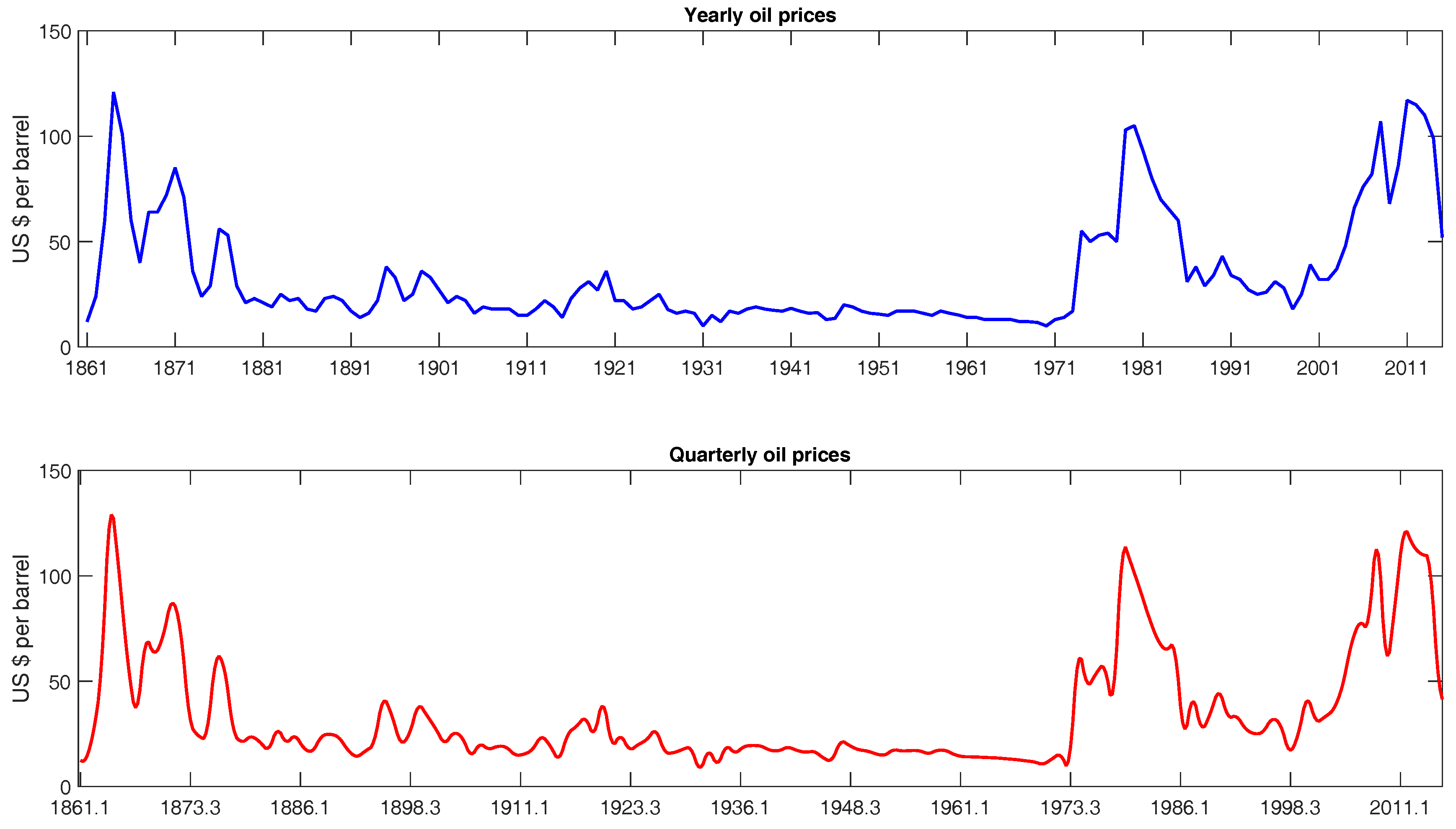
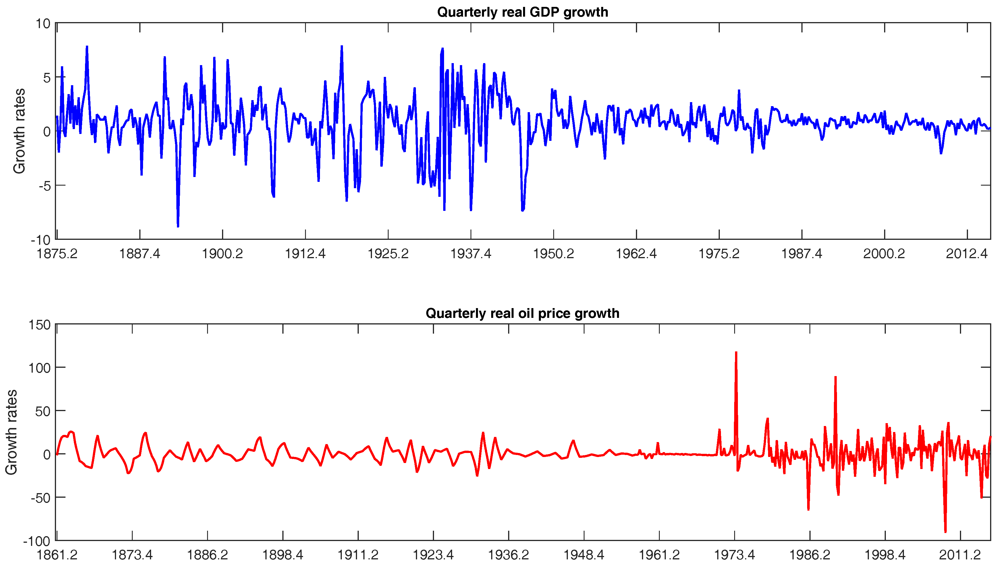
2. Data
3. Univariate Analysis of the Series
3.1. Changes in Mean
3.2. Changes in Volatility
4. Multivariate Analysis of the Series
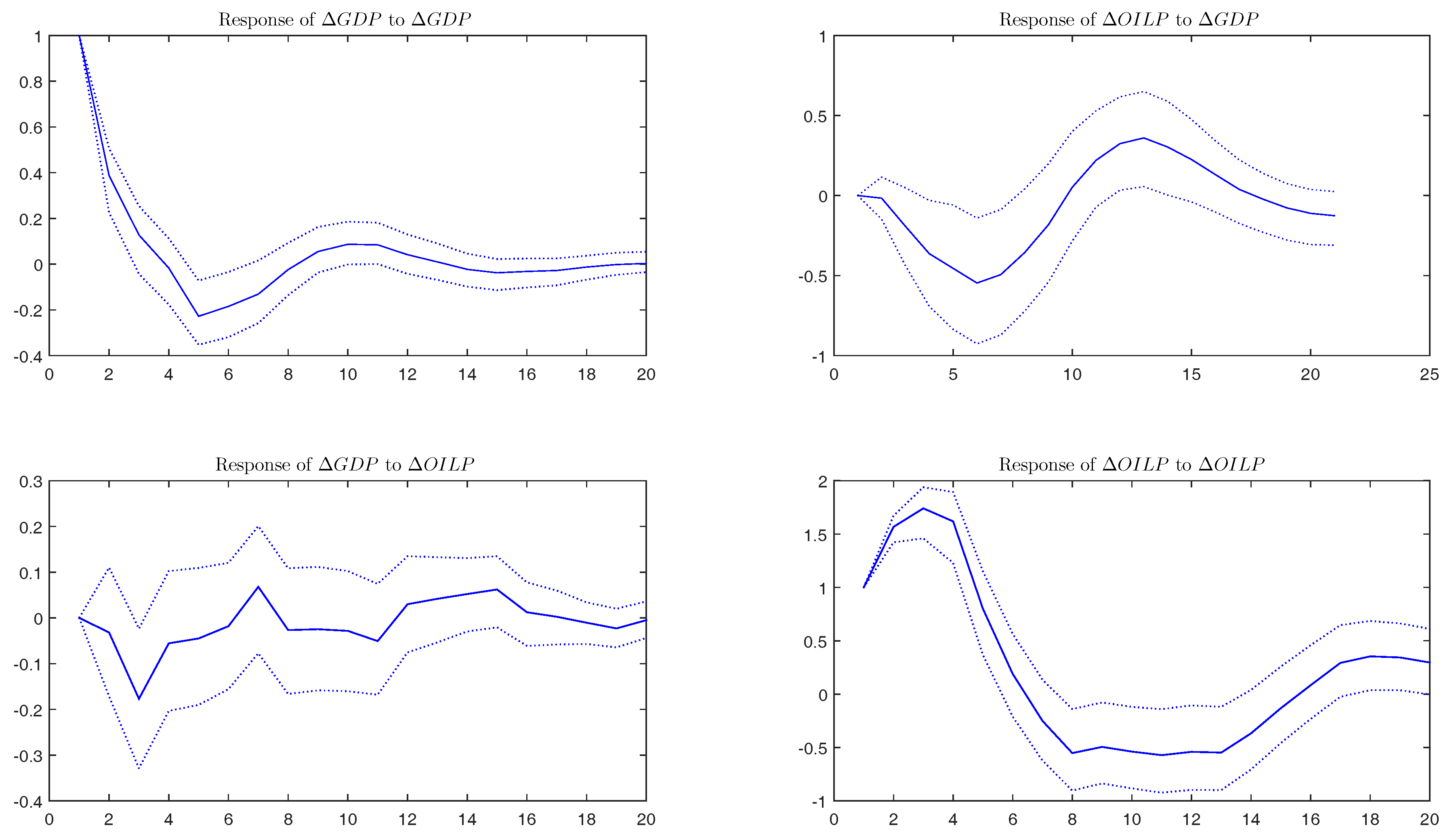
4.1. VAR Estimation
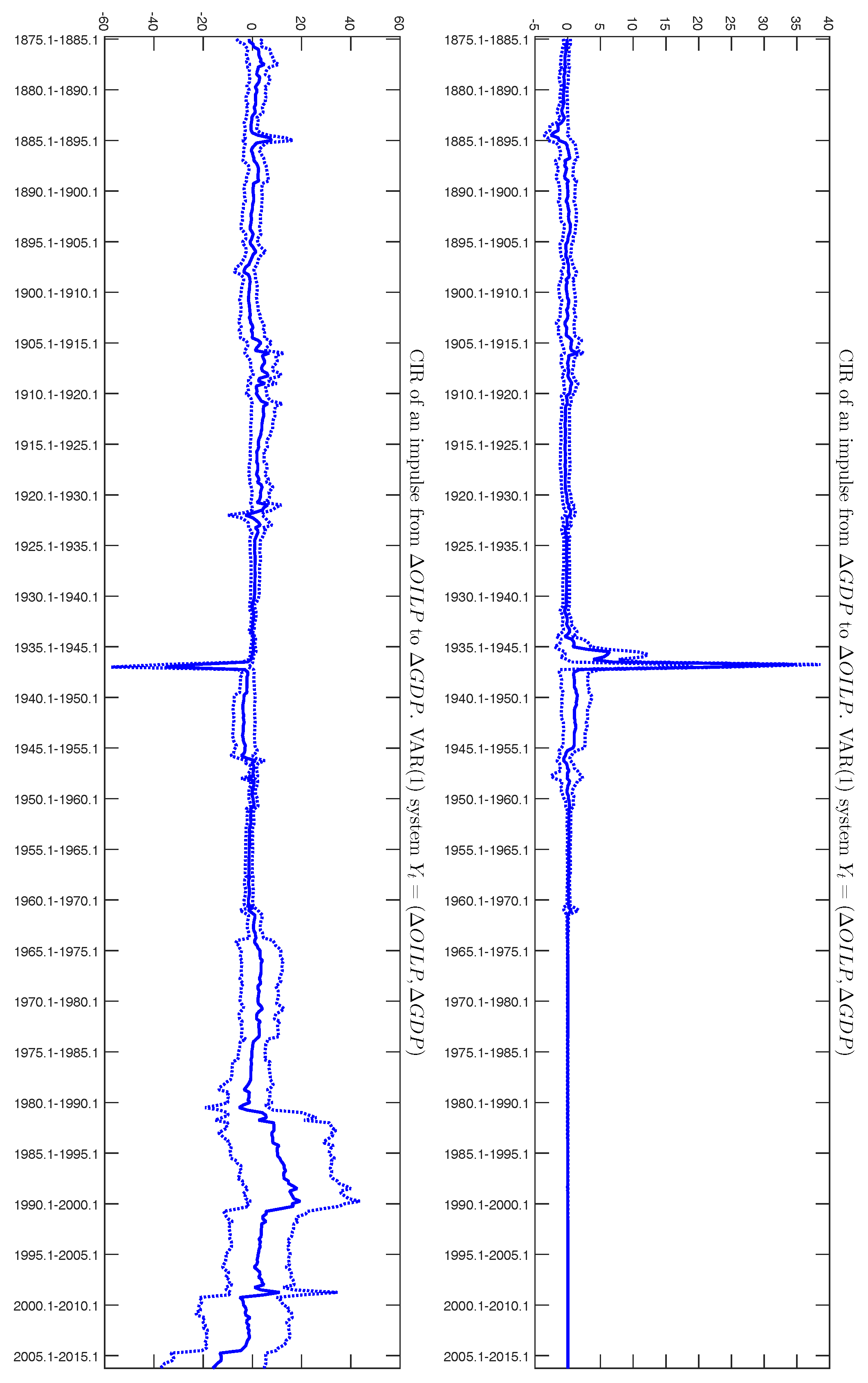
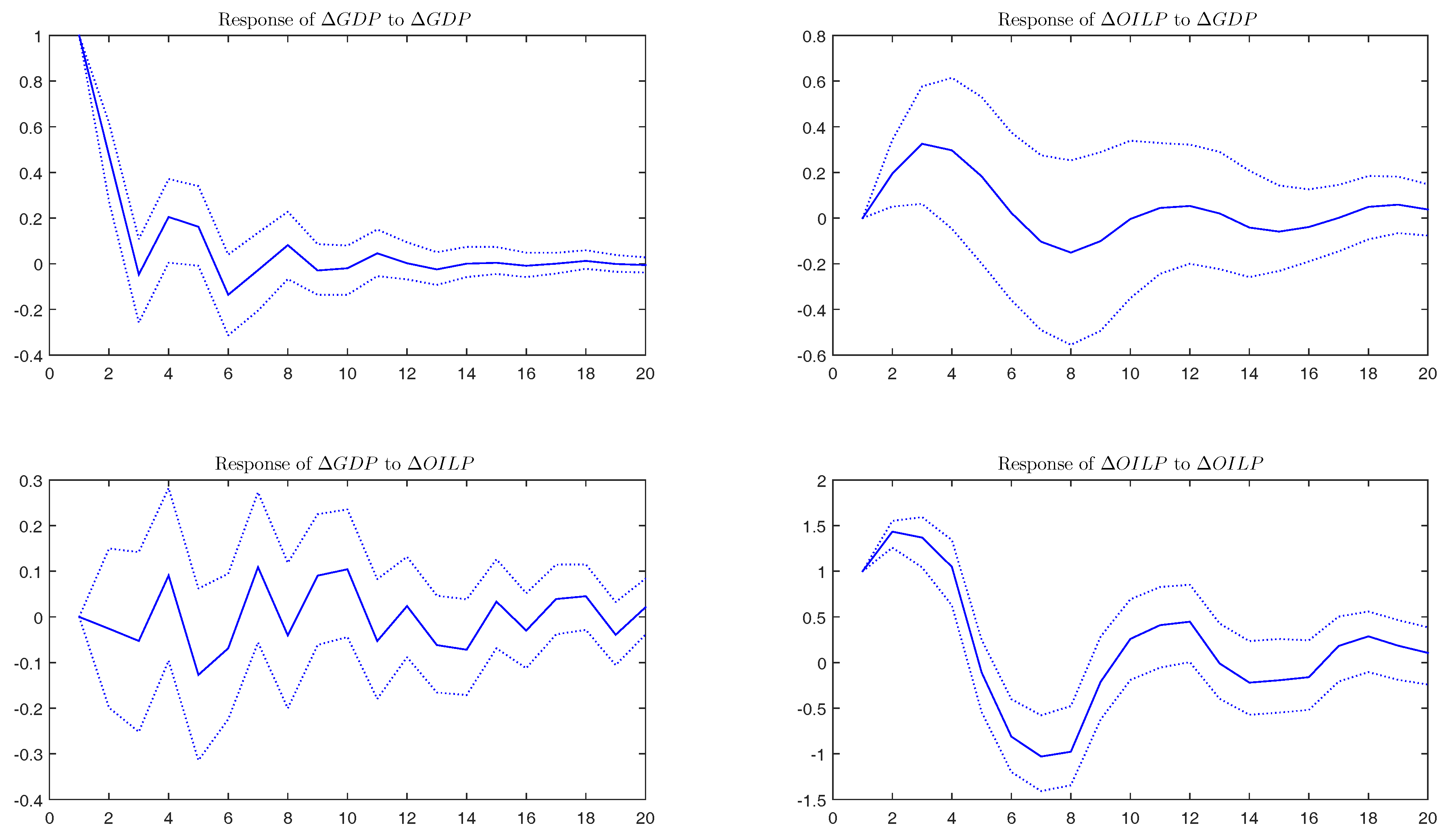
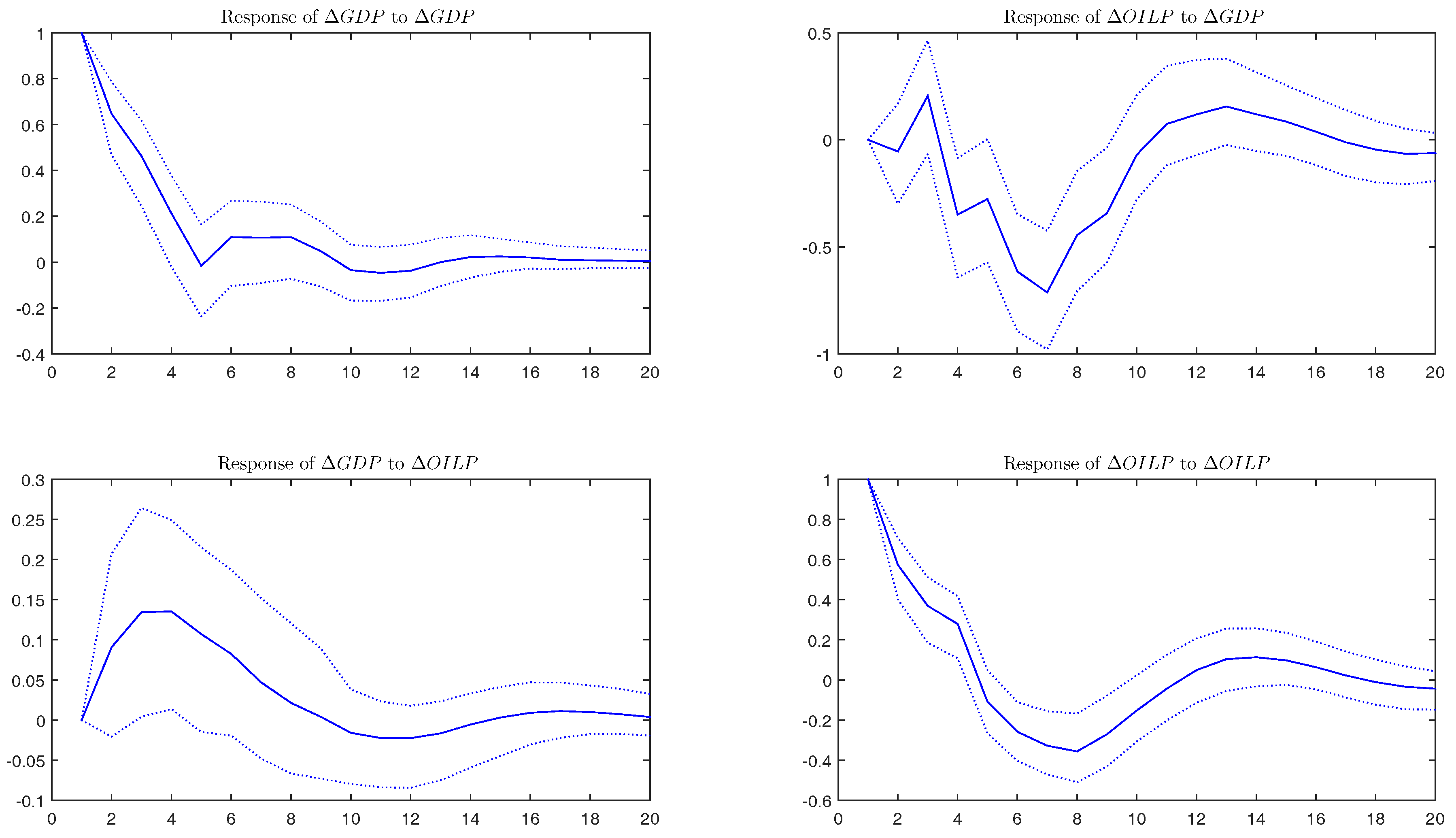
4.2. Rolling Sample Analysis
4.3. Structural Breaks in the Relationship between Oil Prices and GDP
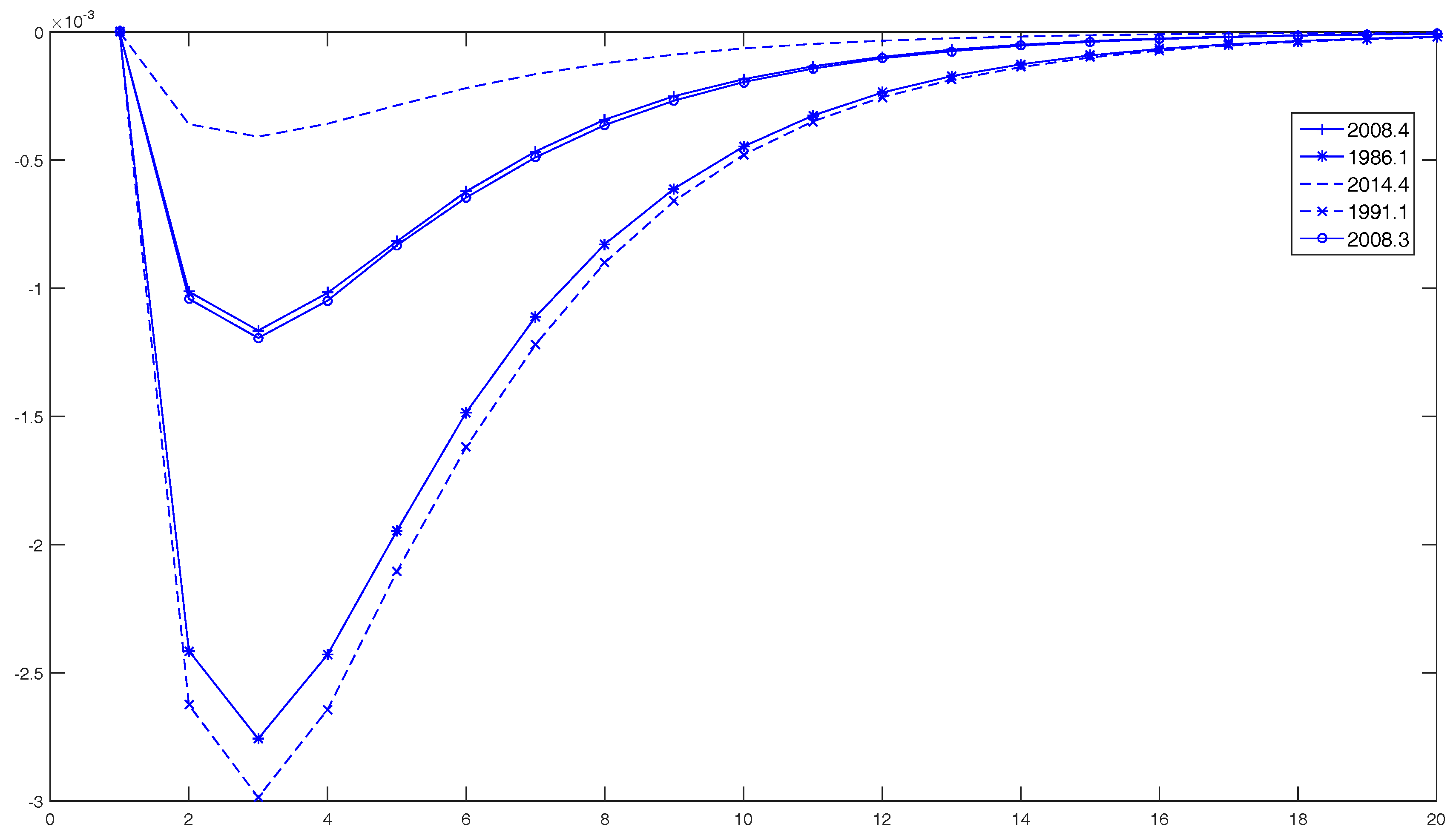
5. A Time-Varying GDP-Oil Price Model
6. Conclusions
Acknowledgments
Author Contributions
Conflicts of Interest
References
- J.D. Hamilton. “Oil and the macroeconomy.” In The New Palgrave Dictionary of Economics. Edited by S.N. Durlauf and L.E. Blume. London, UK: Palgrave Macmillan, 2008. [Google Scholar]
- L. Kilian. “The Economic Effects of Energy Price Shocks.” J. Econ. Lit. 46 (2008): 871–909. [Google Scholar] [CrossRef]
- O.J. Blanchard, and J. Galí. The Macroeconomic Effects of Oil Price Shocks: Why are the 2000s so different from the 1970s? In International Dimensions of Monetary Policy. NBER Chapters; Cambridge, MA, USA: National Bureau of Economic Research, Inc., 2007, pp. 373–421. [Google Scholar]
- A. Gomez-Loscos, M.D. Gadea, and A. Montañés. “Economic growth, inflation and oil shocks: Are the 1970s coming back? ” Appl. Econ. 44 (2012): 4575–4589. [Google Scholar] [CrossRef]
- J.D. Hamilton. “Oil and the Macroeconomy since World War II.” J. Political Econ. 91 (1983): 228–248. [Google Scholar] [CrossRef]
- A. Gómez-Loscos, A. Montañés, and M.D. Gadea. “The impact of oil shocks on the Spanish economy.” Energy Econ. 33 (2011): 1070–1081. [Google Scholar] [CrossRef]
- E. Dvir, and K.S. Rogoff. Three Epochs of Oil. NBER Working Paper; Cambridge, MA, USA: National Bureau of Economic Research, Inc., 2009. [Google Scholar]
- K. Mohaddes, and M.H. Pesaran. “Oil prices and the global economy: Is it different this time around? ” USC-INET Reseach Paper, No. 16-21. 2016. Available online: https://papers.ssrn.com/sol3/papers.cfm?abstract_id=2808084 (accessed on 6 June 2016).
- Z. Qu, and P. Perron. “Estimating and testing structural changes in multivariate regressions.” Econometrica 75 (2007): 459–502. [Google Scholar] [CrossRef]
- R.J. Gordon. The American Business Cycle: Continuity and Change. NBER Book Series Studies in Business Cycles; Cambridge, MA, USA: National Bureau of Economic Research, 1986. [Google Scholar]
- British Petroleum. BP Statististical Review of World Energy. Technical report; London, UK: British Petroleum, 2016. [Google Scholar]
- C. Chow, and A.L. Lin. “Best linear unbiased interpolation, distribution, and extrapolation of time series by related series.” Rev. Econ. Stat. 53 (1971): 372–375. [Google Scholar] [CrossRef]
- J. LeSage. “Applied Econometrics Using MATLAB.” 1999. Available online: http://www.spatial-econometrics.com/html/mbook.pdf (accessed on 9 July 2016).
- E.M. Quilis. “A Matlab library of temporal disaggregation methods.” Instituto Nacional de Estadística, Internal Document, Madrid, Spain, 2004. [Google Scholar]
- J. Bai, and P. Perron. “Estimating and Testing Linear Models with Multiple Structural Changes.” Econometrica 66 (1998): 47–78. [Google Scholar] [CrossRef]
- J. Bai, and P. Perron. “Computation and analysis of multiple structural change models.” J. Appl. Econom. 18 (2003): 1–22. [Google Scholar] [CrossRef]
- J. Bai, and P. Perron. “Critical values for multiple structural change tests.” Econom. J. 6 (2003): 72–78. [Google Scholar] [CrossRef]
- J. Liu, S. Wu, and J. V. Zidek. “On Segmented Multivariate Regressions.” Statistica Sinica 7 (1997): 497–525. [Google Scholar]
- M.D. Gadea-Rivas, A. Gómez-Loscos, and G. Pérez-Quirós. The Great Moderation in Historical Perspective. Is It That Great? CEPR Discussion Paper No. 10825; London, UK: Center for Economic Policy Research, 2014. [Google Scholar]
- D.W.K. Andrews. “Heteroskedasticity and Autocorrelation Consistent Covariance Matrix Estimation.” Econometrica 59 (1991): 817–858. [Google Scholar] [CrossRef]
- C. Inclán, and G.C. Tiao. “Use of Cumulative Sums of Squares for Retrospective Detection of Changes of Variance.” J. Am. Stat. Assoc. 89 (1994): 913–923. [Google Scholar] [CrossRef]
- A. Sanso, V. Arago, and J.L. Carrion-i Silvestre. “Testing for changes in the unconditional variance of financial time series.” Revista de Economia Financiera 4 (2004): 32–53. [Google Scholar]
- A. Deng, and P. Perron. “The Limit Distribution of the Cusum of Squares Test Under General Mixing Conditions.” Econom. Theory 24 (2008): 809–822. [Google Scholar] [CrossRef]
- J. Zhou, and P. Perron. Testing for Breaks in Coefficients and Error Variance: Simulations and Applications. Working Papers Series No. wp2008-010; Boston, MA, USA: Department of Economics, Boston University, 2008. [Google Scholar]
- G. Fagiolo, M. Napoletano, and A. Roventini. “Are output growth-rate distributions fat-tailed? some evidence from OECD countries.” J. Appl. Econom. 23 (2008): 639–669. [Google Scholar] [CrossRef]
- J.D. Hamilton. Historical Oil Shocks. NBER Working Paper No. 16790; Cambridge, MA, USA: National Bureau of Economic Research, Inc., 2011. [Google Scholar]
- A.M. Herrera, and E. Pesavento. “The Decline in U.S. Output Volatility: Structural Changes and Inventory Investment.” J. Bus. Econ. Stat. 23 (2005): 462–472. [Google Scholar] [CrossRef]
- J.H. Stock, and M.W. Watson. Has the Business Cycle Changed and Why? NBER Working Paper No. 9127; Cambridge, MA, USA: National Bureau of Economic Research, Inc., 2002. [Google Scholar]
- M.D. Gadea, A. Gomez-Loscos, and G. Perez-Quiros. The Two Greatest. Great Recession vs. Great Moderation. CEPR Discussion Paper Series No. 10092; London, UK: Center for Economic Policy Research, 2014. [Google Scholar]
- C. Sims. “Macroeconomics and Reality.” Econometrica 48 (1980): 1–48. [Google Scholar] [CrossRef]
- H. Lütkepohl. Introduction to Multiple Time Series Analysis. Berlin, Germany: Springer, 2005. [Google Scholar]
- C. Granger. “Investigating Causal Relations by Econometric Models and Cross Spectral Methods.” Econometrica 37 (1969): 424–438. [Google Scholar] [CrossRef]
- L. Kilian. “Small-Sample Confidence Intervals For Impulse Response Functions.” Rev. Econ. Stat. 80 (1998): 218–230. [Google Scholar] [CrossRef]
- M.D. Gadea, and A. Gomez-Loscos. “Oil price shocks and the US economy: What makes the latest oil price episode different.” Int. Econ. Lett. 3 (2014): 36–44. [Google Scholar]
- G.E. Primiceri. “Time Varying Structural Vector Autoregressions and Monetary Policy.” Rev. Econ. Stud. 72 (2005): 821–852. [Google Scholar] [CrossRef]
- C. Baumeister, and L. Kilian. “Understanding the Decline in the Price of Oil since June 2014.” J. Assoc. Environ. Resour. Econ. 3 (2016): 131–158. [Google Scholar] [CrossRef]
- J.D. Hamilton. “What is an oil shock? ” J. Econom. 113 (2003): 363–398. [Google Scholar] [CrossRef]
- 1.Since the seminal work of [5] for the US economy, a growing number of articles have analyzed the economic consequences of oil price shocks in industrialized countries. Most of the literature shows that the effect of oil price on the economy was very important during the 1970s, but has gradually disappeared since then (many studies support this view; the work in [2] provides a comprehensive review of the literature). The papers [4,6] show that this influence has revived, but with less intensity, since 2000 and, most important, is manifested on inflation.
- 2.The authors find that the real price of oil has historically tended to be both more persistent and more volatile whenever rapid industrialization in the world economy coincided with uncertainty regarding access to supply.
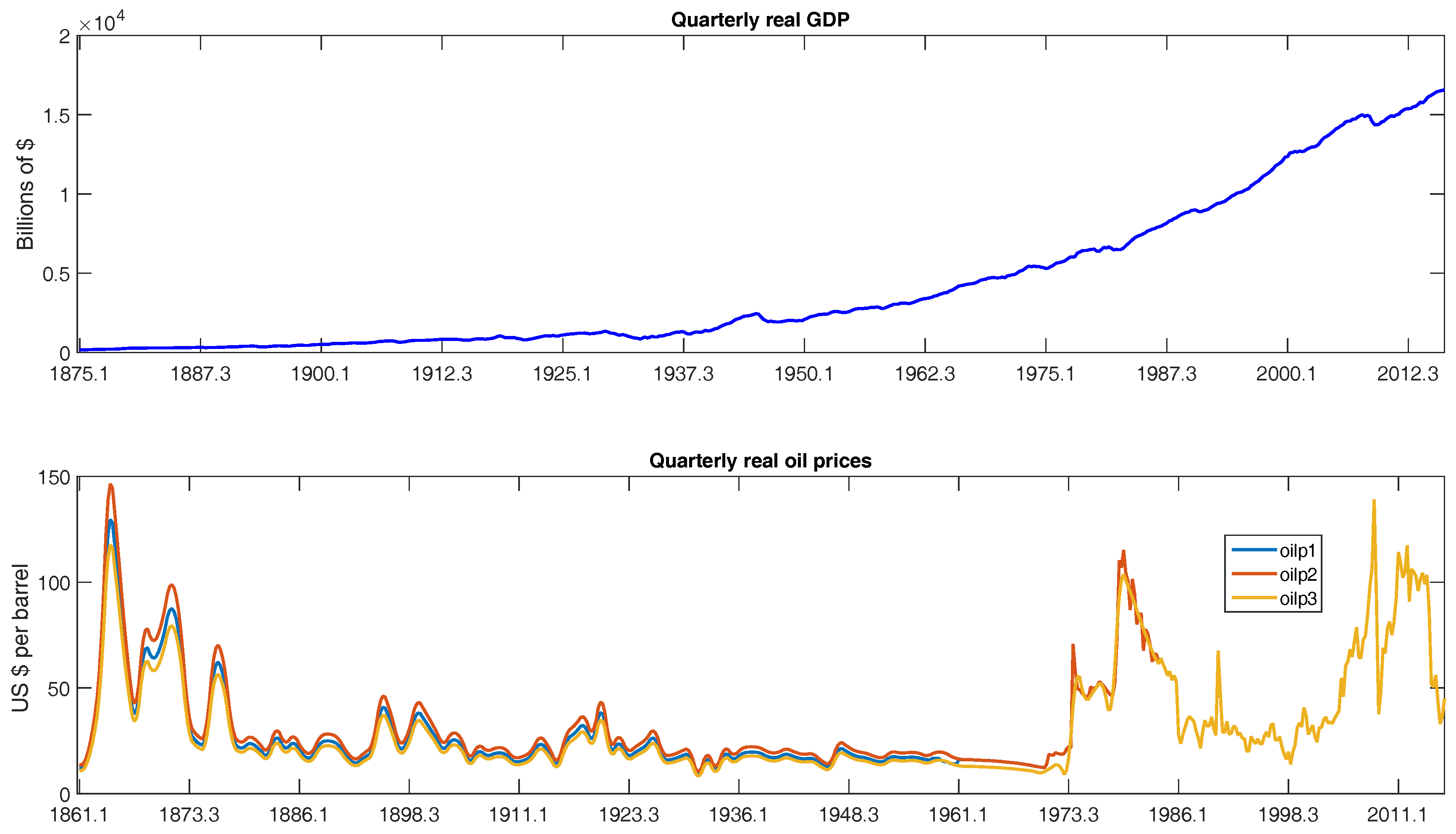
- 3.The first series is in real 2009 dollars, while the long historical series is in real 1972 dollars, but has been transformed to link both. The historical series is taken from Appendix B of [10].
- 4.Chow-Lin interpolation is a regression-based technique to transform low-frequency (annual, in our case) data into higher-frequency (quarterly, in our case) data. In particular, we apply the average version, which disaggregates the annual data into the means of four quarters and is the most suitable approach for price data, and select the maximum likelihood method. We use the Matlab toolbox of [13,14]. This approach gives us the best fit when compared to the available quarterly data. However, we have tested the accuracy of other disaggregation methods and the results remain broadly unchanged.
- 5.Prices are in 2009 US dollars per barrel, and the US GDP deflator data are from the IMF.
- 6.We have also considered other alternatives: (1) use the British Petroleum dataset, updating the last years with the annual Brent series and transforming the whole sample into quarterly data through the Chow-Lin procedure; (2) use the historical British Petroleum series linked to the West Texas Intermediate data or the Producer Price Index for crude petroleum (since they are available or from 1984 onward) instead of Brent prices. We have decided to disregard these options to obtain a more homogeneous dataset by using Brent prices. However, comparing the path of the alternative series to the one we use, we do not observe much difference. Furthermore, we repeated some calculations, obtaining quite similar results.
- 7.We have tested, but not rejected, the hypothesis that both series are I(0), using a battery of standard unit root tests. The stationarity of the series is a pre-condition for applying the BP method. Detailed results are available upon request.
- 8.See [18].
- 9.Alternatively, we tried a standard autoregressive model of order 1, with and , finding similar conclusions. The results are also robust to considering a higher number of maximum breaks. A paper by [19] also confirms the absence of structural breaks in the mean of US GDP series.
- 10.The IT approach is extended to more general processes by [23], showing that the correction for non-normality proposed by [22] is suitable when the test is applied to the unconditional variance of raw data. Furthermore, [24] carry out a Monte Carlo experiment that highlights the adequacy of this procedure when the mean or other coefficients in the regression do not change; otherwise, the test has important size distortions, which increase with the magnitude of change in the mean.
- 11.The US GDP growth rates can be approximated by leptokurtic densities as shown by [25]. This indicates that output growth changes tend to be quite uneven in the sense that large positive or negative changes seem to be more frequent than a Gaussian model would predict.
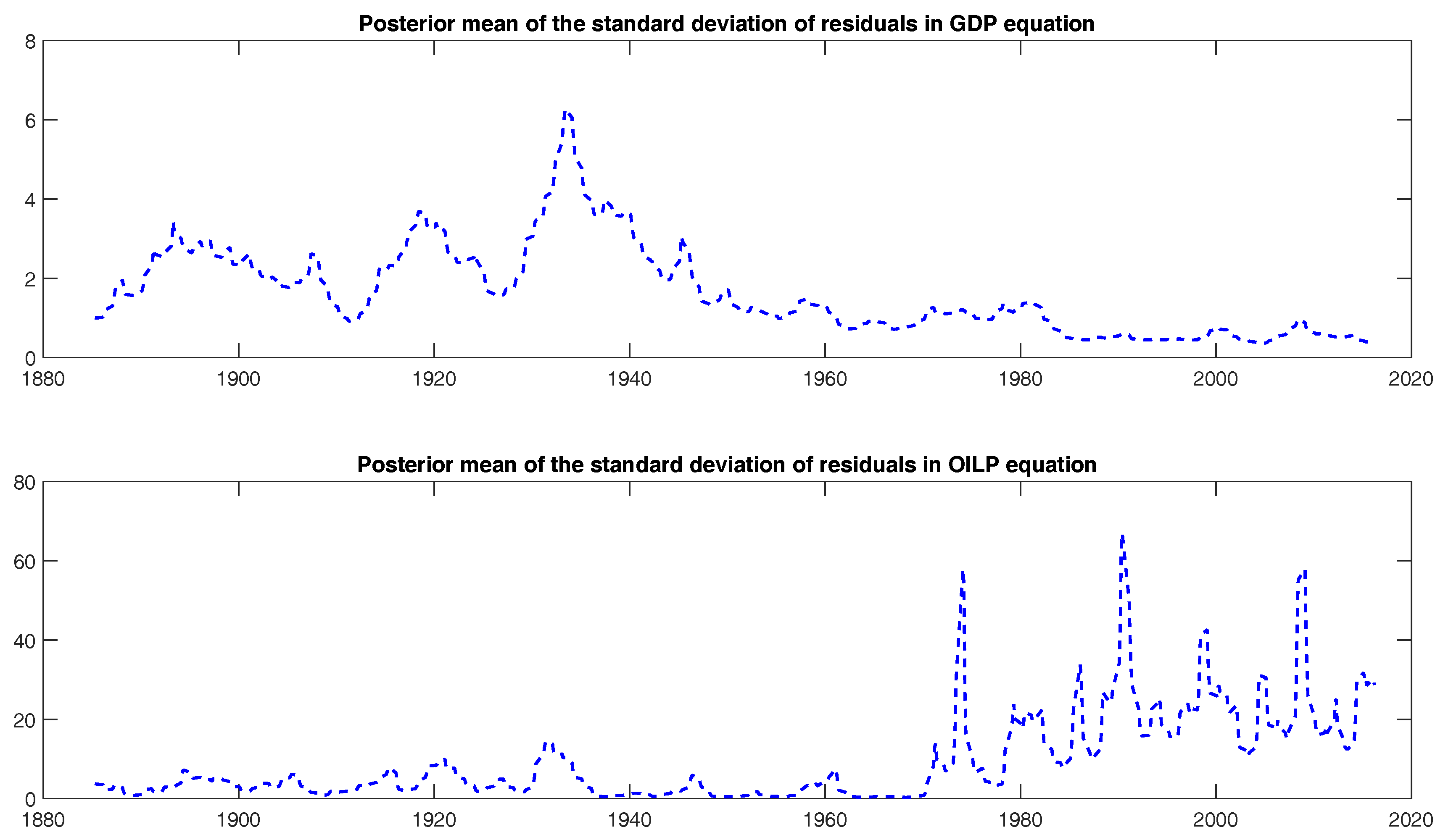
- 12.The authors offer a thorough analysis of the sources and features of these different volatility periods.
- 13.Construction of the first long-distance pipeline began in 1878, allowing the railroad monopoly over oil transportation to end. However, US control over excess exploitable reserves ended and OPEC dominance increased in 1969.
- 14.See also [26] for a historical survey of the oil industry with particular focus on the events related to significant oil price changes.
- 15.A paper by [24] shows that, in case changes in the mean of the series are not taken into account, the test suffers from severe size distortions. However, we have shown that our series do not have structural breaks in the mean. This method has been used in several studies: [27,28,29], among others.
- 16.Notice that these break points are the least significant ones with both approaches. Indeed, the break of March 1929 is not even identified with Model 2 of the BP methodology.
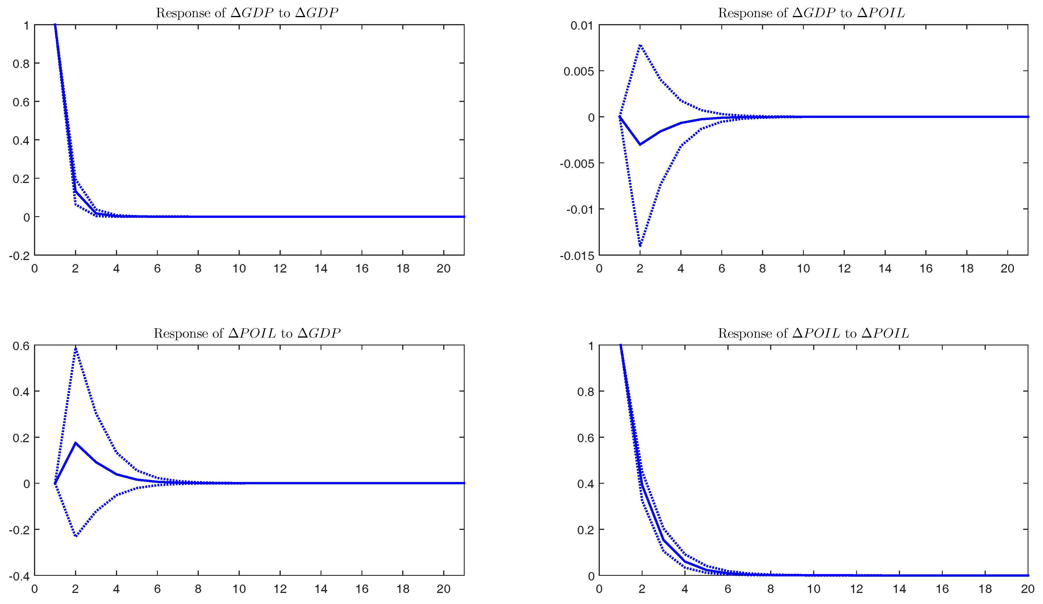
- 17.The SBIC criterion selects one lag. Nevertheless, other information criteria, such as the Akaike information criterion (AIC) and the Hannan-Quinn (HQ) criterion select five lags. Therefore, we use a VAR(1) as the preferred model and estimate, additionally, a VAR(5) to check the robustness of our results. For simplicity, and to save space, we only present the results for the VAR(1) and discuss whether some interesting results or significant differences appear with respect to the VAR(5).
- 18.We have repeated the analysis with annual data as a robustness check, finding qualitatively the same results.
- 19.An estimation of a VAR system with five lags does not change this conclusion.
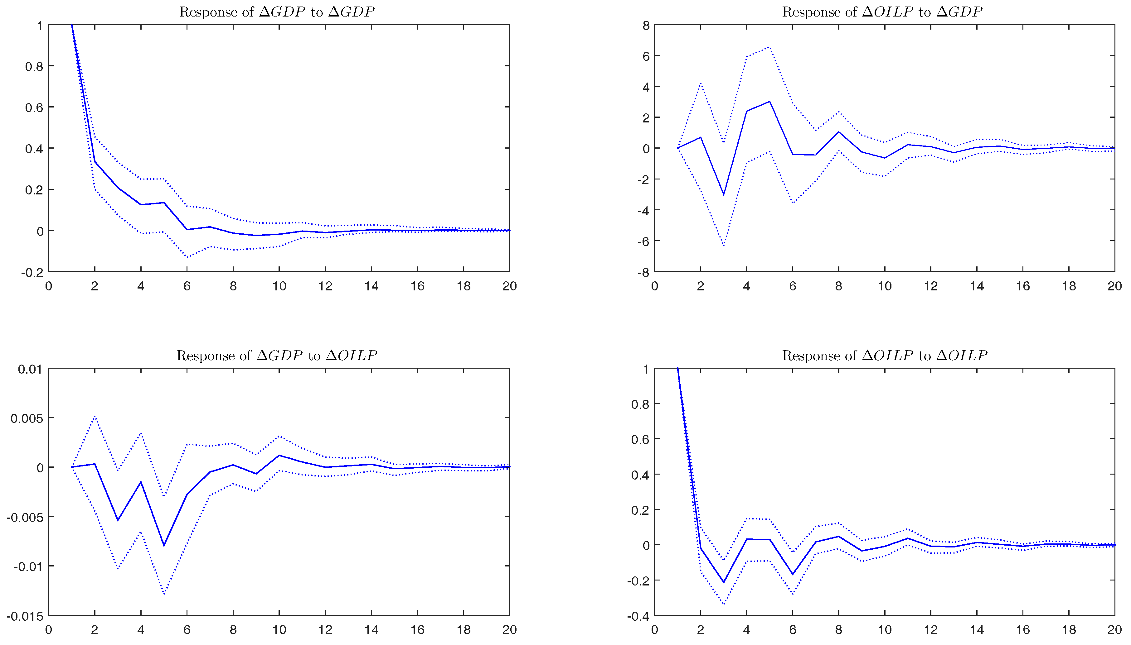
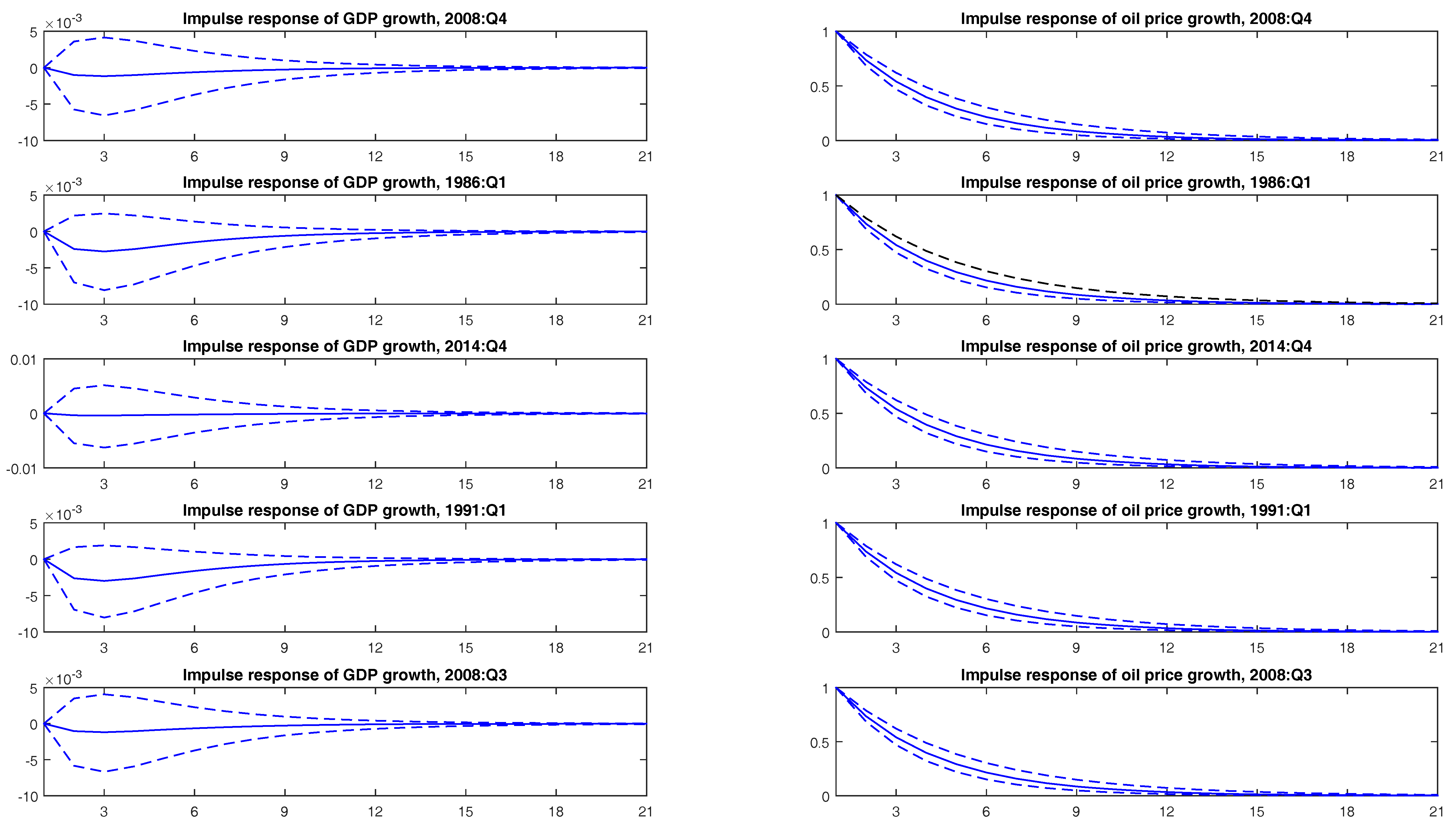
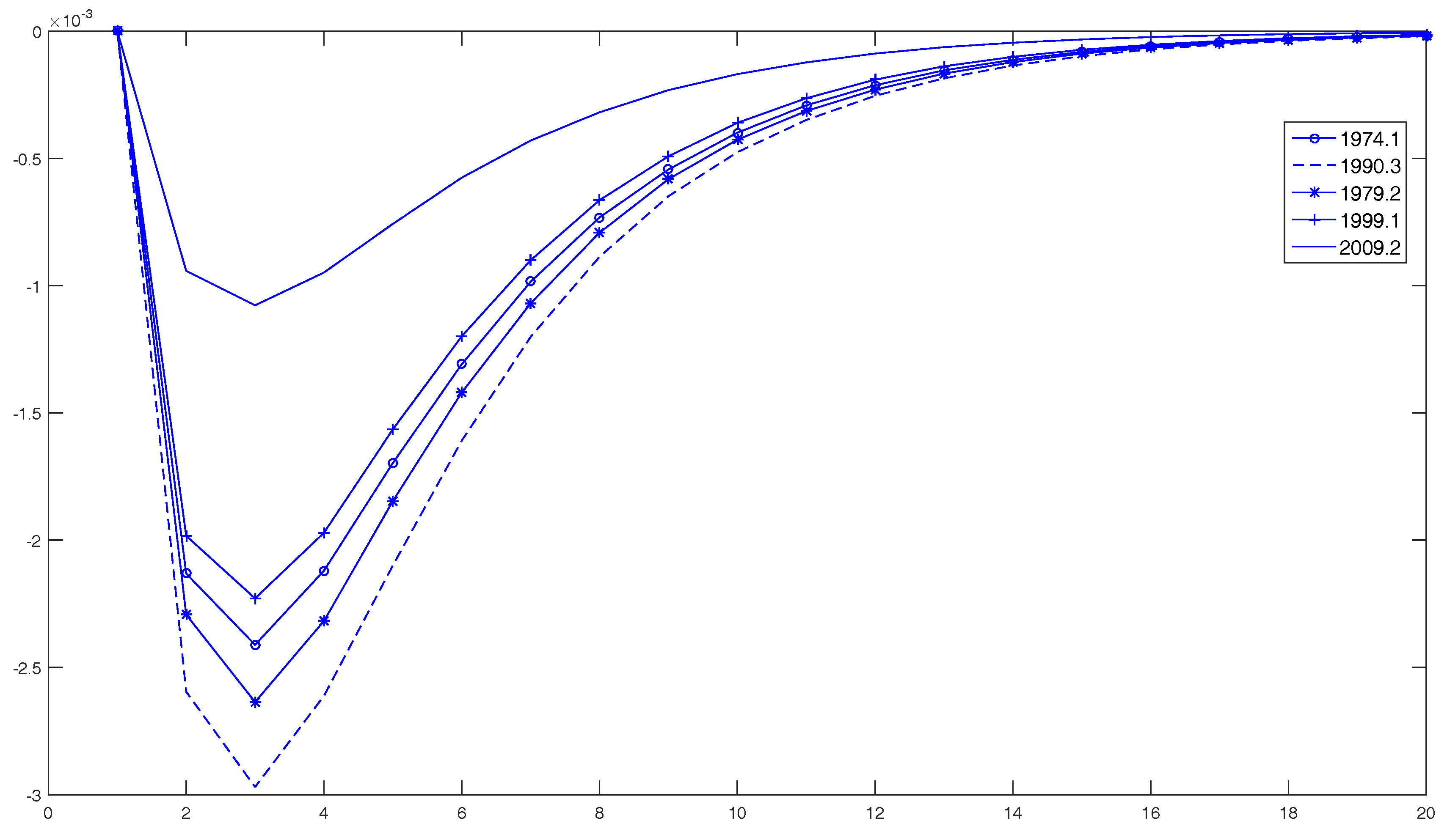
- 20.As is well-known, the order of variables is relevant for IRF computation, as the Cholesky decomposition requires triangulation. To test the robustness of the results, we have redone all calculations with the system in the inverse order: and have also calculated the generalized IRF. The findings are the same, which is not surprising, given the results of casualty.
- 21.The confidence intervals are (−0.0269, 0.0151) and 0.3306 (−0.4279, 1.1086), respectively. They were computed with the same bootstrap methodology as for the IRFs.
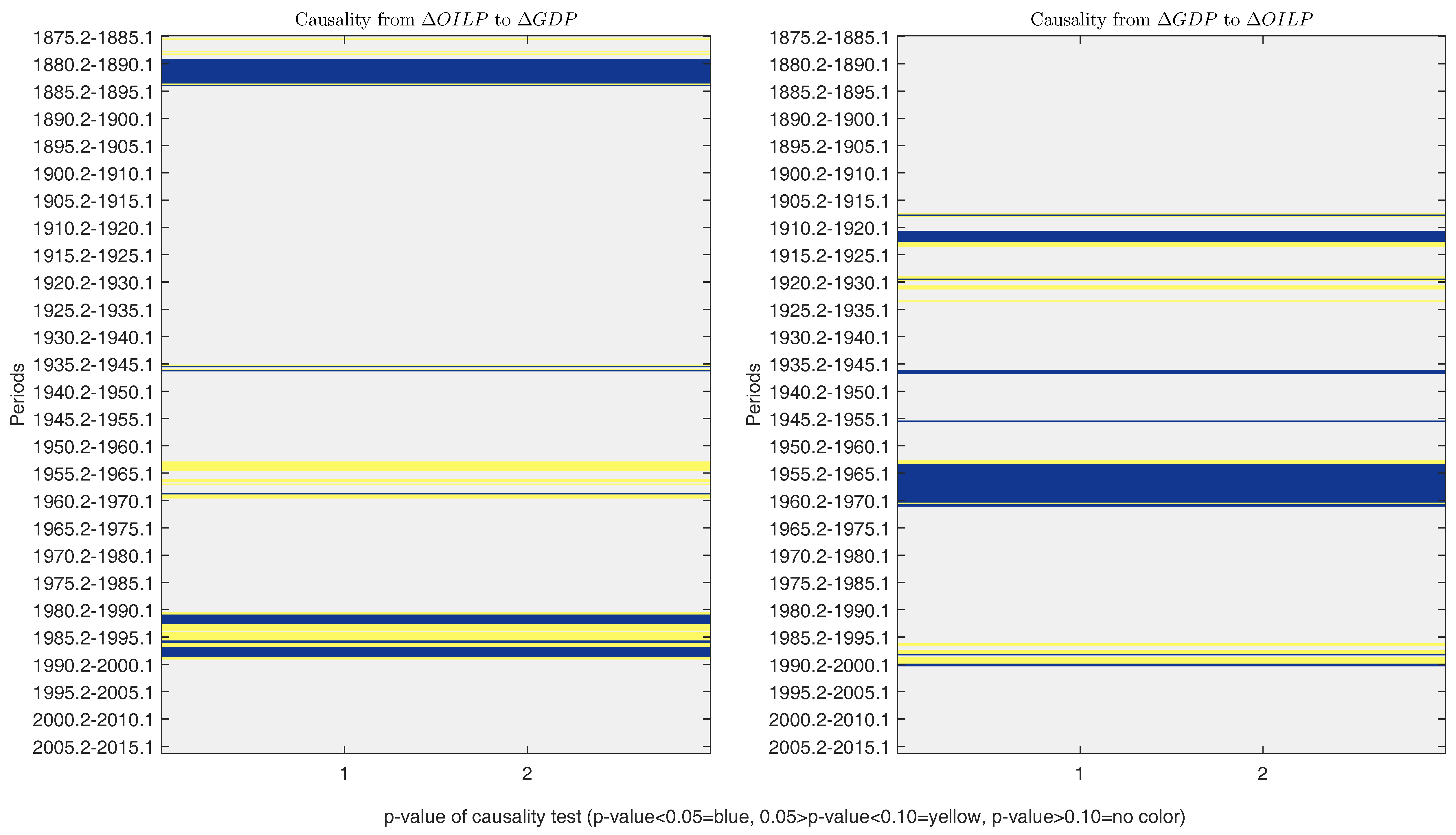
- 22.Since 2005, the causality test is near the 10% threshold limit of significance. This result agrees with that of [34], who document a positive and significant effect of GDP growth on oil prices since the 2000s.
- 23.This was an extraordinary growth period in the US economy. The increasing demand for oil caused oil price increases.
- 24.During this period, the US economy had to face World War II with devastating economic consequences (the first postwar US recession began at the end of 1948). The demand for petroleum products caused a sharp increase in the price of oil and although the US increased oil production enormously during World War II, there were shortages in several plants.
- 25.We have repeated the analysis using annual data, reaching the same conclusions.
- 28.The Arab-Israel war in 1973, which followed the long-lasting Arab-Israeli conflict, and the Iranian revolution in 1978–1979 are a few examples.
- 29.Such as the Iran-Iraq war of 1980–1988, the Persian Gulf War of 1990–1991, the Venezuelan crisis of 2002, the Iraq War of 2003, or the Libyan uprising of 2011.
- 30.For technical details, see [35]. An adaptation of its Matlab code has been used to compute the estimates.
- 31.These results confirm those obtained by [19].
- 32.The Great Recession has been the worst recession in the US economy since the Great Moderation. For an analysis of the Great Moderation in the face of the Great Recession, see [29].
- 33.See [36] for a thorough analysis of this episode.
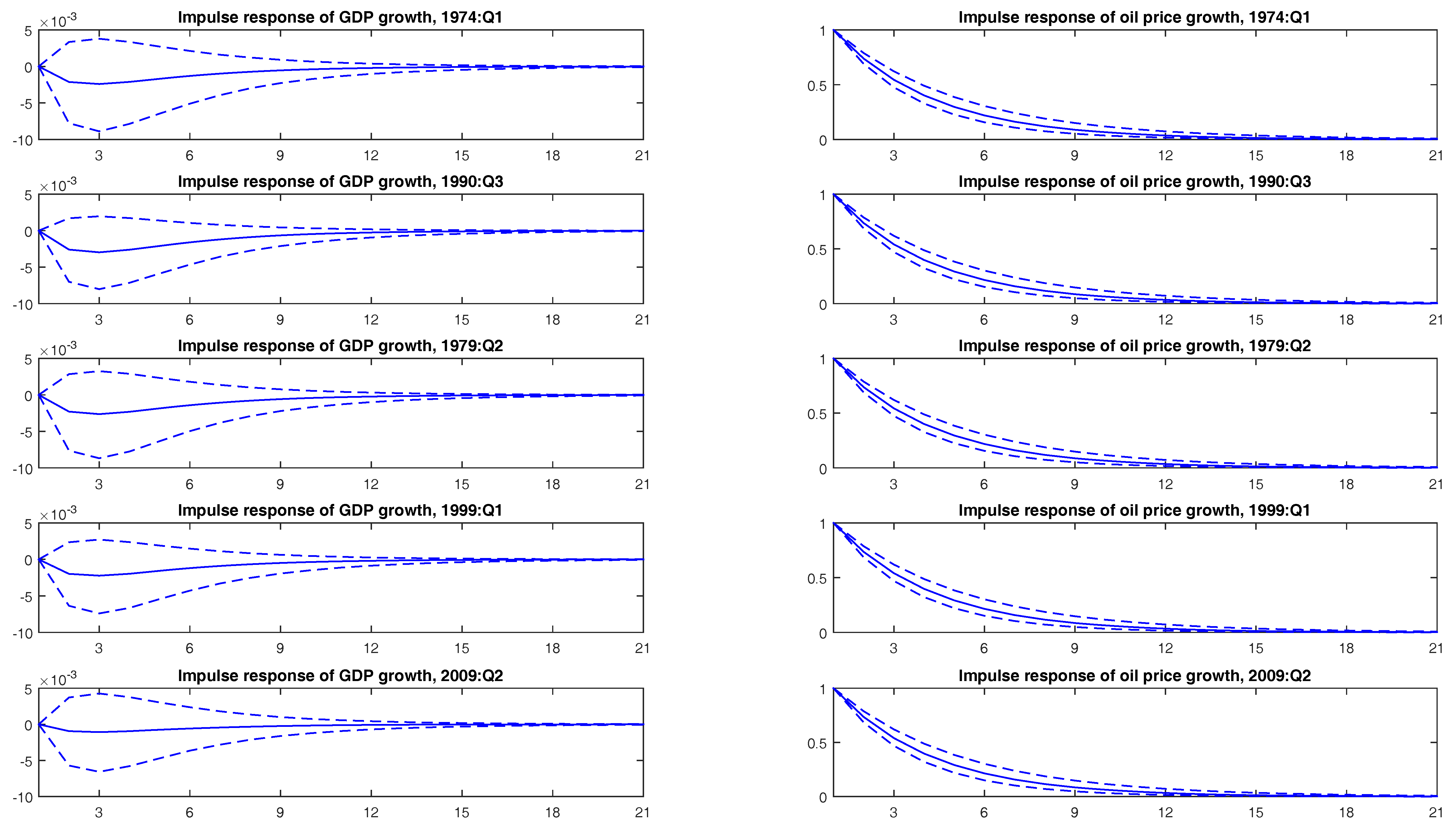
- 34.These results would be in line with [3], who find a changing relationship over time, such that the economy is more resilient to an oil price shock today than in the past.


| ΔGDP | ΔPOIL | |
|---|---|---|
| supF(k) | ||
| k = 1 | ||
| k = 2 | ||
| k = 3 | ||
| k = 4 | ||
| k = 5 | ||
| supF(l + 1/l) | ||
| l = 0 | ||
| l = 1 | ||
| l = 2 | ||
| l = 3 | ||
| l = 4 | − | − |
| UDmax | ||
| WDmax | ||
| T(SBIC) | 0 | 0 |
| T(LWZ) | 0 | 0 |
| T(sequential) | 0 | 0 |
| ΔGDP | ΔOILP | |
|---|---|---|
| ICSS(IT) | ||
| April 1917 | April 1878 | |
| February 1946 | February 1914 | |
| February 1984 | March 1921 | |
| April 2007 | March 1930 | |
| February 2009 | February 1934 | |
| March 1936 | ||
| April 1944 | ||
| March 1947 | ||
| April 1960 | ||
| April 1970 | ||
| ICSS | ||
| March 1929 | January 1862 | |
| March 1934 | January 1963 | |
| February 1946 | April 1878 | |
| January 1984 | March 1930 | |
| February 1934 | ||
| April 1973 | ||
| ICSS | ||
| April 1917 | April 1878 | |
| February 1946 | April 1973 | |
| January 1984 |
| ΔGDP | ΔOILP |
|---|---|
| Model 1 | |
| March 1929 | April 1878 |
| January 1947 | February 1935 |
| February 1984 | April 1973 |
| Model 2 | |
| March 1946 | March 1973 |
| April 1983 | |
| Coeff. | p-Value | |
|---|---|---|
| Dependent variable: ΔGDP | ||
| Intercept | 0.486 | 0.000 |
| ΔGDP | 0.392 | 0.000 |
| ΔOILP | −0.003 | 0.649 |
| Dependent variable: ΔOILP | ||
| Intercept | −0.049 | 0.932 |
| ΔGDP | 0.175 | 0.478 |
| ΔOILP | 0.132 | 0.002 |
| Granger causality | ||
| ΔOILPGDP | 0.207 | 0.649 |
| ΔGDPPOIL | 0.504 | 0.478 |
| WDmax | SupLR | Seq(l + 1/l) | TBi | |||
|---|---|---|---|---|---|---|
| 0 vs. 1 | 0 vs. 2 | 0 vs. 3 | ||||
| 979.130 | 979.130 | 1104.231 | 1159.779 | 156.685 | 64.157 | April 1912, January 1941, March 1970 |
| Granger-Wald causality test | ||||||
| February 1875–April 1912 (6) | January 1913.1–January 1941 (6) | February 1941–March 1970 (5) | April 1970–February 2016 (5) | |||
| ΔOILPGDP | 0.481 | 0.339 | 0.400 | 0.100 | ||
| ΔGDPOILP | 0.251 | 0.272 | 0.000 | 0.497 | ||
© 2016 by the authors; licensee MDPI, Basel, Switzerland. This article is an open access article distributed under the terms and conditions of the Creative Commons Attribution (CC-BY) license ( http://creativecommons.org/licenses/by/4.0/).
Share and Cite
Gadea, M.D.; Gómez-Loscos, A.; Montañés, A. Oil Price and Economic Growth: A Long Story? Econometrics 2016, 4, 41. https://doi.org/10.3390/econometrics4040041
Gadea MD, Gómez-Loscos A, Montañés A. Oil Price and Economic Growth: A Long Story? Econometrics. 2016; 4(4):41. https://doi.org/10.3390/econometrics4040041
Chicago/Turabian StyleGadea, María Dolores, Ana Gómez-Loscos, and Antonio Montañés. 2016. "Oil Price and Economic Growth: A Long Story?" Econometrics 4, no. 4: 41. https://doi.org/10.3390/econometrics4040041
APA StyleGadea, M. D., Gómez-Loscos, A., & Montañés, A. (2016). Oil Price and Economic Growth: A Long Story? Econometrics, 4(4), 41. https://doi.org/10.3390/econometrics4040041