Market Microstructure Effects on Firm Default Risk Evaluation

Abstract

Default probability is a fundamental variable determining the credit worthiness of a firm and equity volatility estimation plays a key role in its evaluation. Assuming a structural credit risk modeling approach, we study the impact of choosing different non parametric equity volatility estimators on default probability evaluation, when market microstructure noise is considered. A general stochastic volatility framework with jumps for the underlying asset dynamics is defined inside a Merton-like structural model. To estimate the volatility risk component of a firm we use high-frequency equity data: market microstructure noise is introduced as a direct effect of observing noisy high-frequency equity prices. A Monte Carlo simulation analysis is conducted to (i) test the performance of alternative non-parametric equity volatility estimators in their capability of filtering out the microstructure noise and backing out the true unobservable asset volatility; (ii) study the effects of different non-parametric estimation techniques on default probability evaluation. The impact of the non-parametric volatility estimators on risk evaluation is not negligible: a sensitivity analysis defined for alternative values of the leverage parameter and average jumps size reveals that the characteristics of the dataset are crucial to determine which is the proper estimator to consider from a credit risk perspective.

1. Introduction

Many empirical works in the financial literature highlight the poor performance of structural credit risk models for defaultable bonds in predicting default probabilities and credit spreads, especially when considering very short maturities. The classical approach to firm’s value models is the one proposed by Merton [1]: a firm’s equity and debt are studied as contingent claims partitioning the total value of the firm; the underlying assets value dynamic is defined by a geometric Brownian motion. The empirical evidence indicates that classical standard structural models still have some difficulties in accurately explaining default rates and spreads simultaneously. Estimation or calibration methods provide evidence that predicted credit spreads are far below observed ones [2], the structural variables explain little of the credit spread variation [3], pricing error is large for corporate bonds [4]. From an econometric point of view, the calibration of these models on real data is non trivial due to key variables which are not directly observable: the underlying firm’s asset value and the volatility of firm’s asset value returns. This critical issue concerning the calibration of the underlying asset dynamics becomes even more problematic when one wants to consider also market microstructure effects into the structural modeling framework. The market microstructure literature strongly indicates that trading noises can affect equity prices so that the estimation of equity volatility and other related quantities may become a very difficult task. Observed equity prices can diverge from their equilibrium value due to illiquidity, asymmetric information, price discreteness and other measurement errors. Among many others, the works by [5,6] study the effects of trading noise on the optimal sampling frequency of observed equity prices since sparse sampling may reduce the bias in volatility measures due to such microstructure effects. The aim is to use as much as possible the information content of high-frequency noisy equity prices and define a procedure to back out the firm’s asset volatility.

In the specific context of structural credit risk models, the relationship between the unobservable asset volatility and the observed equity value predicted by the pricing model is masked by trading noise; ignoring microstructure effects could non-trivially inflate estimates for the “true” equity volatility, and this would lead to poor estimates for spreads and default rates. This issue has been analyzed in [7], where the authors extend [8] to explicitly account for trading noise contamination on equity prices: they devise a particle filter-based maximum likelihood method based solely on the time series of observed equity values, showing its robustness with respect to market microstructure effects. The importance of using high frequency data to back out parameters involved in firm’s value dynamics has been highlighted in [9]: the authors propose a novel approach to identify the volatility and jump risks components of individual firms from high-frequency observed equity prices, arguing that these new measures can allow to capture the effects of stochastic volatility and jumps in the firm’s underlying asset dynamics ([3,10]). Their analysis suggests that high-frequency-based volatility measures can help to better explain credit spreads, above and beyond what is already captured by the true leverage ratio. However, the highest frequency considered in this paper is the 5-min conservative sampling frequency which allows to filter microstructure effects. Recently, several non-parametric estimators of daily stock volatility have been proposed, allowing to exploit the information content of intra-day high-frequency data without being affected by microstructure effects [5,6,11,12,13,14,15].

In this paper, we carry on the analysis in [16] considering a structural approach à la Merton (see [1]) for defaultable corporate bonds in the presence of market microstructure noise and study a class of models for the underlying firm’s assets value dynamics allowing for: (i) stochastic asset return volatility; (ii) jump component. This extension to stochastic volatility and jump component for the underlying assets is deemed to be particularly significant from a credit risk modeling perspective: indeed, pricing and hedging issues related to equity markets suggest that stochastic volatility and jumps are crucial in order to improve credit spreads predictions. In addition to this, a negative leverage effect between stock prices and volatility is a typical feature observed in real data: stock prices tend to decrease when volatility rises.

The mathematical framework for a firm’s assets value process is defined through, alternatively, Heston [17] and Bates [18] models; as particular cases, the classical Merton model [1] and Merton model with jumps in the underlying asset dynamics [19] can also be derived. We propose a particular econometric approach to structural models calibration based on a non-parametric estimation of equity volatility from high-frequency intra-day equity prices. Market microstructure effect is introduced by assuming equity prices contaminated by trading noise under two different scenarios: (a) trading noise independent log-Gaussian distributed; (b) trading noise correlated with intra-day equity log-returns. From both an econometric and credit risk point of view, the interest of the analysis is concentrated on three key variables: equity volatility, underlying (unobservable) asset volatility, default probability. The aim of the paper is to exploit the information content of intra-day high-frequency prices and compare the performance of alternative non-parametric equity estimators in filtering out microstructure effects, retrieve the underlying asset volatility and thus evaluate the corresponding predicted default probabilities under the historical measure. The estimated underlying asset volatility is obtained as result of a specific calibration procedure matching the actual default probability (for a given maturity) and considering equity volatility estimation as input: this technique allows us to overcome the problem of its non-observability even when dealing with a structural approach. The results of our Monte Carlo simulation analysis highlight that asset volatility and default probabilities are deeply affected by the choice of the non-parametric estimator for equity volatility. From an econometric point of view, the commonly used 5-min Realized Volatility estimator is unable to provide reliable estimates for equity volatility in the presence of market microstructure noise, leading to a significant underestimation of both asset volatility and default probabilities and causing a wrong prediction of the real firm’s risk profile. Obviously, the Realized Volatility estimator based on noisy 1-min returns would provide even worse estimates, thus confirming results already discussed in [16]. For this reason, in this paper we discuss full results for the 5-min Realized Volatility estimator providing a more fair benchmark for all the other estimates. The Monte Carlo analysis has been developed for firms belonging to A rating class, revealing that the choice of the non-parametric volatility estimator has a strong influence on risk evaluation. This confirms the results of the analysis in [16] and extends their validity to the case of stochastic volatility models with jump components for the firm’s assets.

The paper also provides empirical evidence highlighting the relevance of this study from a practical credit risk perspective: the idea underlying the empirical analysis is to consider high frequency equity prices of a US company and the corresponding time series of credit default swap (CDS) premium as direct measure of a firm’s default probability (see also [9]). A regression analysis between daily CDS quotes and the corresponding volatility measures based on high-frequency intra-day equity prices is performed to show that alternative non parametric equity volatility measures can have a different explanatory power and thus a different impact for a firm default probability evaluation.

The paper is organized as follows: Section 2 describes the alternative non-parametric estimation techniques for equity volatility considered in our paper. Section 3 provides empirical evidence related to the role of equity volatility estimates based on high-frequency equity prices for default probability evaluation. Section 4 defines the structural credit risk model. Section 5 reports the results of our Monte Carlo analysis for backing out assets volatility and evaluating default probabilities. Section 6 analyzes the sensitivity of the asset volatility calibration and default probability estimation w.r.t. increasing levels of the leverage effect and of the jump component. Finally, Section 7 concludes.

2. Non-Parametric Volatility Estimation under Microstructure Noise

This section describes the approach we follow to estimate the equity volatility ${\Sigma }_t^s$ from high-frequency equity data and gives details about the implementation of the specific volatility measures considered in our analysis. We set ${\tilde{p}}_t:=log{\tilde{S}}_t$, the noisy equity log-price. Time is measured in daily units. We build daily measure of volatility by considering daily windows of n intra-day equity data ${\tilde{p}}_{t,j}$, $j=1,\dots ,n$. Besides the well known Realized Volatility estimator ${\Sigma }_t^{RV}:={\sum }_{j=1}^n{\delta }_j{\left(\tilde{p}\right)}^2$, where ${\delta }_j\left(\tilde{p}\right):={\tilde{p}}_{t,j}-{\tilde{p}}_{t,j-1}$ is the j-th within-day equity log-return on day t, we consider the following estimators of the volatility process ${\Sigma }_t^s$: the bias corrected estimator by Hansen and Lunde [12]

$${\Sigma }_t^{HL}:={\Sigma }_t^{RV}+2\frac{n}{n-1}\sum _{j=1}^{n-1}{\delta }_j\left(\tilde{p}\right){\delta }_{j+1}\left(\tilde{p}\right);$$

the flat-top realized kernels by [6,20]

$${\Sigma }_t^K:=\sum _{h=-H}^{H}k\left(\frac{h}{H+1}\right)\sum _{j=\left|h\right|+1}^n{\delta }_j\left(\tilde{p}\right){\delta }_{j-\left|h\right|}\left(\tilde{p}\right).$$

with kernels of $T{H}_2$ type $k\left(x\right)={sin}^2\left(\frac{\pi }{2}{(1-x)}^2\right)$. The realized kernels may be considered as unbiased corrections of the Realized Volatility by means of the first H autocovariances of the returns. In particular, when H is selected to be zero the realized kernels become the Realized Volatility. Our analysis includes also the two-scale estimator by [15]

$${\Sigma }_t^{TS}:=\frac{S}{S-1}\left(\frac{1}{S}\sum _{s=1}^S{\Sigma }_t^{G^{\left(s\right)}}-\frac{1}{S}{\Sigma }_t^{RV}\right).$$

The two-scale (subsampling) estimator is a bias-adjusted average of lower frequency realized volatility computed on S non-overlapping observation sub-grids $G^{\left(s\right)}$ containing $n_S$ observations. Recently, [13] proposed a pre-averaging technique as an alternative to sub-sampling in order to reduce the microstructure effects. The idea is that if one averages a number of observed log-prices, one is closer to the latent process $p\left(t\right)$. This approach, when well implemented, gives rise to rate optimal estimators of power variations. In particular, a consistent estimator of the integrated volatility can be constructed as

$${\Sigma }_t^{PA}=\frac{\sqrt{\Delta }}{\theta {\psi }_2}\sum _{s=0}^{n-k_n+1}{\overline{\delta }}_s{\left(\tilde{p}\right)}^2-\frac{{\psi }_1\Delta }{2{\theta }^2{\psi }_2}\sum _{s=1}^n{\delta }_s{\left(\tilde{p}\right)}^2,$$

where the pre-averaged return process is given by

$${\overline{\delta }}_s\left(\tilde{p}\right):=\sum _{r=1}^{k_n}g\left(\frac{r}{k_n}\right){\delta }_{s+r}\left(\tilde{p}\right)=\frac{1}{k_n}\left(\sum _{j=k_n/2}^{k_n-1}{\tilde{p}}_{t,s+j}-\sum _{j=0}^{k_n/2-1}{\tilde{p}}_{t,s+j}\right),$$

$\theta =k_n\sqrt{\Delta }$, ${\psi }_1=1$ and ${\psi }_2=1/12$, corresponding to the "hat" weight function $g\left(x\right)=x\wedge (1-x)$. The Fourier-Fejer estimator [14] is given by

$${\Sigma }_t^F=\frac{{\left(2\pi \right)}^2}{N+1}\sum _{s=-N}^N\left(1-\frac{\left|s\right|}{N}\right)c_s\left(d{\tilde{p}}_n\right)c_{-s}\left(d{\tilde{p}}_n\right),$$

where $c_k\left(d{\tilde{p}}_n\right)=\frac{1}{2\pi }{\sum }_{i=1}^{n}exp(-\mathrm{i}k{t}_{i-1}){\delta }_i\left(\tilde{p}\right)$.

Finally, the jump-robust Bipower Variation [21] is defined as

$${\Sigma }_t^{BV}={\mu }_1^{-2}\sum _{j=2}^n|{\delta }_{j-1}\left(\tilde{p}\right)\left|\right|{\delta }_j\left(\tilde{p}\right)|,$$

with ${\mu }_1\simeq 0.7979$.

Finite sample MSE-based optimal rules for choosing the parameters employed by these estimators are discussed in [15,22,23,24]. Here, we proceed according to the following rules: a simple approximation of the optimal sampling frequency for the Realized Volatility and Bipower Variation estimators is to choose the number of observations approximately equal to $n^{*}={(Q/4E{\left[{\eta }^2\right]}^2)}^{1/3}$, where Q is the integrated quarticity estimated by means of low frequency returns. The optimal number of sub-grids S is given by $c^{*}{n}^{2/3}$, where $c^{*}={(Q/48E{\left[{\eta }^2\right]}^2)}^{-1/3}$. For the Kernel estimator, we apply the optimal mean square error bandwidth selection suggested by [23] and get $H=c^{*}{\xi }^{4/5}{n}^{3/5}$, where $c^{*}={(144/0.269)}^{1/5}$, ${\xi }^2=E\left[{\eta }^2\right]/\sqrt{Q}$. In the case of the Pre-averaging estimator, inspired by [23], we choose $k_n=c^{*}{\xi }^{4/5}{n}^{3/5}$. Finally, for the Fourier-Fejer estimator, the optimal cutting frequency N can be easily obtained by direct minimization of the estimated MSE given by Theorem 3 in [24].

3. Empirical Evidence

The aim of this section is to provide empirical evidence that alternative non parametric equity volatility estimates constructed from high-frequency equity return data may have different impact on a firm default probability evaluation. The idea is to consider high frequency equity prices of a US company and the corresponding time series of CDS quotes. We choose to use the CDS premium as a direct measure of a firm’s default probability as already done in [9]. The CDS is one of the most popular instrument in the credit derivatives market. Under a CDS contract, the protection seller promises to buy the reference bond at its par value when a predefined default event occurs. In return, the protection buyer makes periodic payments to the seller until the maturity date of the contract or until a credit event occurs. This periodic payment is called the CDS spread and provides a pure measure of the default risk of the reference entity. Indeed, if compared with corporate bond spreads, CDS spreads provide relatively ”pure” pricing of the default risk of the underlying entity and are typically traded on standardized terms. Moreover, bond spreads are more likely to be affected by differences in contractual arrangements, such as differences related to seniority, coupon rates, embedded options, guarantees and liquidity factors, which do not necessarily reflect the ”pure” default risk of the underlying asset. Finally, CDS spreads tend to respond more quickly to changes in credit conditions in the short run, which may be partly due to the absence of funding and short-sale restrictions in the derivatives market.

We adopt equity volatility measures as proxies for the time variation in volatility risk of a firm in order to examine the relationship between equity returns and credit spreads. The empirical results in [9] suggest that the volatility risk alone can predict up to 48% of the variation in CDS spread levels, particularly for investment-grade entities. Their analysis was based on a sample of US corporates over the period January 2001–December 2003.

Here we focus on 5-year CDS contracts for the Dow Jones Alcoa company. The sample covers the period from 10 November 2015 to 23 May 2016, for a total of 134 trading days. Our CDS quotes are daily and are provided by Bloomberg. The corresponding equity price sample contains 52,166 observations at a 1-min frequency for a 6.5 h daily trading period.

Table 1. Summary statistics of the 1-min transaction data on equity prices for the Alcoa company in the period from 10 November 2015 to 23 May 2016 (52,166 trades). ”Std. Dev.” denotes the sample standard deviation of the variable.

Variable	Mean	Std. Dev.	Min	Max
AA US Equity price	9.02	1.05	6.15	11.49
log-return (%)	1.68 × 10${}^{-4}$	1.78 × 10${}^{-1}$	−4.66 × 10${}^0$	3.73 × 10${}^0$

and

Table 2. Summary statistics of the daily CDS premium data (basis points) for Alcoa company in the period from 10 November 2015 to 23 May 2016. ”Std. Dev.” denotes the sample standard deviation of the variable.

Variable	Mean	Std. Dev.	Min	Max
CDS premium	433.87	91.09	329.24	661.63

report, respectively, descriptive statistics of high frequency equity prices and CDS premium in our dataset.

High-frequency equity returns are contaminated by transaction costs, bid-ask bounce effects and possibly jumps leading to biases in the variance measures. Figure 1 shows the time plot of the 1-min log-returns and the autocorrelation function. Row data exhibit a strongly significant negative first order autocorrelation and higher order autocorrelations remain significant up to lag 12. Sparse sampling at 5 min frequency eliminates most of the microstructure effects. Figure 2 shows the histogram of the 1-min equity log-returns. We can see that the distribution of returns is far from being normal. Skewness is equal to –1.2078, while kurtosis is 73.1947.

Jumps have been identified and measured using the Threshold Bipower Variation method (TBV) of [25], which is based on the joint use of Bipower variation and threshold estimation. This method provides a powerful test for jump detection, which is employed at the significance level of 99.99%. This procedure allows to identify a total of 25 days with jumps which are removed from the sample. Since the TBV estimator is not robust to microstructure noise, we compute this measure of the integrated volatility in the presence of jumps using sparse sampling.

A first empirical evidence of the correlation between CDS spreads and equity volatility measures can be obtained by visually inspecting Figure 3, that shows the time plot of the daily 5-years CDS spreads in basis points (bottom panel) and the corresponding equity Realized Volatility (top panel) for our sample of 109 days after jump removal. The final sample covers the period 10 November 2015–23 May 2016. As we can observe from the figure, CDS spreads increased substantially in the middle of the considered period and gradually declined at the end of the sample period. The (annualized) daily return volatility varies between 0.2016 and 1.0838 following a similar pattern. From a statistical point view, the CDS spread and Realized Volatility series are correlated with positive correlation of $61.7\%$ that exactly reflects their common qualitative behavior.

In order to examine the explanatory power of the different equity volatility measures introduced in Section 2, for each estimated series of equity integrated volatility, we project the CDS spread on day t on a constant and the corresponding estimated daily volatility measure ${\Sigma }_t^s$. The Mincer-Zarnowitz evaluation regression takes the form

$$CD{S}_t={\varphi }_0+{\varphi }_1{\Sigma }_t^s+{ϵ}_t,$$

(1)

where $t=1,\dots ,109$. The $R^2$ from these regressions provides a direct assessment of the variability in the CDS premium that is explained by the particular estimates in the regressions. The $R^2$ can therefore be interpreted as a simple gauge of the explanatory power of the volatility estimate and hence of its potential economic significance.

Table 3. OLS estimates from regressions (1) of the 5-year CDS spread (%) on day t over a constant and each corresponding equity volatility estimate obtained by estimators defined in Section 2. Standard deviation and T-statistics are reported in brackets.

Estimator	$\widehat{{\varphi }_0}$	$\widehat{{\varphi }_1}$	$R^2$
${\Sigma }_t^{RV}$	2.5476	4.0915	0.3810
Std. Dev.	(0.2312)	(0.5042)
T-statistics	(11.0173)	(8.1155)
${\Sigma }_t^{TS}$	2.0615	4.9657	0.4118
Std. Dev.	(0.2715)	(0.5737)
T-statistics	(7.5916)	(8.6556)
${\Sigma }_t^{HL}$	2.4268	4.4108	0.3884
Std. Dev.	(0.2418)	(0.5350)
T-statistics	(10.0355)	(8.2447)
${\Sigma }_t^K$	2.5293	4.2330	0.3797
Std. Dev.	(0.2340)	(0.5229)
T-statistics	(10.8107)	(8.0944)
${\Sigma }_t^{PA}$	2.6140	4.3276	0.3635
Std. Dev.	(0.2314)	(0.5535)
T-statistics	(11.2956)	(7.8184)
${\Sigma }_t^F$	1.9735	5.1398	0.4236
Std. Dev.	(0.2749)	(0.5796)
T-statistics	(7.1788)	(8.8677)
${\Sigma }_t^{BV}$	2.5891	4.1263	0.3801
Std. Dev.	(0.2267)	(0.5094)
T-statistics	(11.4188)	(8.1010)

shows the OLS estimates from regressions (1). All the estimators are constructed using 1-min returns. The only exceptions are the Realized Volatility and the Bipower Variation, obtained from sparse sampled 5-min returns. All the estimated coefficients are significant at the 0.1% significance level. The signs of coefficients are correct, since a higher equity volatility estimate raises credit spread, and the magnitudes are sensible: for instance, a volatility shock of 1% in the Realized Volatility estimate raises the credit spread by 4%.

As we can observe from the results reported in Table 3, a significant portion of the CDS premium can be explained by the equity volatility estimates. This empirical evidence confirms the key role played by high-frequency equity prices in the evaluation of a firm default probability. The general outcome of our empirical study confirms the results already stated by [9] highlighting the key role of the information content of equity volatility and extends them from an econometric point of view, covering a bigger set of equity volatility estimators besides the 5-min Realized Volatility. Regardless of the specific method implemented to estimate the volatility, we show that the portion of CDS premium variability explained by equity volatility is between 36% and 42%. This smaller percentage w.r.t. the 48% found in [9] should be linked to the differences in market conditions between the two samples considered in the empirical case study.

The commonly used 5-min Realized Volatility yields a $R^2$ of 38%, while estimators robust to microstructure effects can yield higher $R^2$ using all available data. In particular, the Fourier estimator and the Two-scale estimator provide the highest $R^2$ results at 42% and 41%, respectively, with a gain of 10% over the Realized Volatility.

4. Firm Value Model in the Presence of Market Microstructure Noise

This Section describes our structural modeling framework and the model we use to describe trading noise on high-frequency equity data. We consider a stylized Merton-type [1] structural approach that incorporates stochastic volatility and jumps in the presence of market microstructure noise. Firm’s asset value process is defined through a jump-diffusion model, including Bates [18] and Heston [17] models as described in Section 4.1. Market microstructure is considered in our setting through the assumption of equity prices being contaminated by trading noise under two different scenarios: a) independent log-Gaussian distributed noise process, b) trading noise process correlated with intra-day equity log-returns; Section 4.2 gives a full description of market microstructure.

4.1. Assets Value Dynamics and Default Assumptions

We assume the structural credit risk modeling approach defined by Merton [1] and follow the intuition of [3] introducing stochastic volatility and jumps in the underlying firm’s asset value dynamics as

$$\begin{array}{c}{\displaystyle \frac{d{A}_t}{A_t}=(\mu -\delta -\lambda {\mu }_J)dt+\sqrt{V_t}d{W}_t^1+J_{t}d{q}_t}\hfill \\ d{V}_t=k(\theta -V_t)dt+\sigma \sqrt{V_t}d{W}_t^2,\hfill \end{array}$$

(2)

where $A_t$ is firm value, μ is the instantaneous asset return, δ the asset payout ratio. The asset jump component has a Poisson mixing Gaussian distribution, where $q_t$ is a Poisson process with intensity λ and $log(1+J_t)$ are Normally distributed jump sizes in the logarithmic firm value, with expectation $log(1+{\mu }_J)-{\sigma }_J^2/2$ and variance ${\sigma }_J^2$. The Poisson process $q_t$ is independent of the Brownian motions and the jump sizes.The asset return variance, $V_t$, follows a square-root process with long-run mean θ, mean reversion speed k and volatility-of-volatility parameter σ. Finally, ρ is the correlation between Brownian motions $W_t^1,W_t^2$. This dynamics has been studied in the equity-option price literature ([18,26]), while the general credit risk modeling framework has been analyzed by [10]. The model (2) includes the Heston model [17], Merton setting with a jump component [19] and also the original Merton framework [1] by assuming $V_t$ constant through time (i.e., $k,\theta ,\sigma =0$). The firm has two classes of outstanding claims: equity and a zero-coupon debt with promised payment B at maturity T. To be suitable for pricing corporate debt, we adopt the following bankruptcy assumptions from the classical setting [1]: (i) there is only one outstanding bond, i.e., a zero-coupon bond with a promised payment B at maturity; (ii) default can occur only at bond maturity with debt face value as default boundary; and (iii) when default occurs, the absolute priority rule prevails. The payoffs to debt holders and equity holders at time T become, respectively

$$D_T=min(A_T,B),S_T=max(A_T-B,0).$$

From now on, the focus of our study is concentrated on equity value and default probabilities in order to develop our computational econometric analysis. Using no-arbitrage arguments, equity price, namely $S_t$, can be computed as the price of a European call option written on the underlying asset $A_t$ with maturity T

$$S_t=A_t{F}_1^{*}-B{e}^{-r(T-t)}{F}_2^{*},$$

(3)

where $F_i^{*}=F_i^{*}(A_t,V_t;T,B)$$i=1,2$ are the so called risk-neutral probabilities, computed using the corresponding characteristic function (see [17,18]).

We apply Itô’s lemma and get the following specification for equity price dynamics

$$\begin{array}{c}\frac{d{S}_t}{S_t}=\frac{1}{S_t}{\mu }_t(·)dt+\frac{A_t}{S_t}\frac{\partial S_t}{\partial A_t}\sqrt{V_t}d{W}_t^1+\frac{1}{S_t}\frac{\partial S_t}{\partial V_t}\sigma \sqrt{V_t}d{W}_t^2\\ +\frac{1}{S_t}[S_t(A_t(1+J_t),V_t;\Omega )-S_t(A_t,V_t;\Omega )]d{q}_t,\end{array}$$

where ${\mu }_t(·)$ is the instantaneous equity return under the historical probability measure, Ω is the parameter vector. Let ${\Sigma }_t^s$ indicate the instantaneous volatility of log-equity price given by

$${\Sigma }_t^s=\sqrt{{\left(\frac{A_t}{S_t}\right)}^2{\left(\frac{\partial S_t}{\partial A_t}\right)}^2{V}_t+{\left(\frac{\sigma }{S_t}\right)}^2{\left(\frac{\partial S_t}{\partial V_t}\right)}^2{V}_t+2\rho \sigma \frac{A_t}{S_t^2}\frac{\partial S_t}{\partial A_t}\frac{\partial S_t}{\partial V_t}{V}_t}.$$

(4)

Notice that the evolution of equity volatility is driven by two time-varying factors, $A_t$ and $V_t$, while the underlying asset volatility is only driven by $V_t$. As particular case, if asset volatility is constant ($v:=\sqrt{V}$), then Equation (4) reduces to the standard Merton (see [1]) formula ${\Sigma }_t^s=\frac{A_t}{S_t}\frac{\partial S_t}{\partial A_t}v$. The jump size of log-equity price is given by

$$J_t^s=log\left[S_t(A_t(1+J_t),V_t;\Omega )\right]-log\left[S_t(A_t,V_t;\Omega )\right].$$

The firm’s probability of default at maturity T is the probability of $A_T$ being below the constant barrier represented by the face value of debt B. Under the physical probability measure this can be computed through

$$P(A_T<B|A_t)=1-P(A_T\ge B|A_t)=1-F_2(A_t,V_t;T,B),$$

(5)

where $F_2(A_t,V_t;T,B)$ will be evaluated with the historical drift for asset returns.

4.2. Market Microstructure Noise on High-Frequency Equity Prices

Let us consider an individual firm: we can obtain a time series of equity prices $\{S_{t_j},j=1,\dots ,n\}$, with a given constant sampling interval $h=t_j-t_{j-1}$. If one could observe the efficient (i.e., not contaminated by noise) equity price, than equity volatility could be estimated by the well known Realized Volatility estimator [27] at any desired accuracy level using high frequency data. However, as stressed by [7], the relationship between the unobserved asset and the observed equity value predicted by the pricing formula (3) may be masked by trading noise in reality. Econometric literature suggests that observed equity prices can diverge from their equilibrium value due to illiquidity, asymmetric information, price discreteness and other measurement errors. Thus, the approach used to estimate equity volatility must take into account the presence of trading noise affecting the sample of observations.

In this paper we assume an additive error structure for the trading noise on the logarithmic equity value as follows

$$log{\tilde{S}}_{t_j}=log{S}_{t_j}+{\eta }_{t_j},$$

(6)

where the random shocks ${\eta }_{t_j}$, for $0\le j\le n$ are i.i.d. random variables with zero mean and bounded fourth moment and independent from the efficient log-return process. The assumption of independence can be relaxed by considering a particular form of dependent noise, given by [12], with market microstructure noise that is time-dependent in tick time and correlated with efficient returns

$${\tilde{\eta }}_j:=\alpha [log{S}_{t_j}-log{S}_{t_{j-1}}]+{\eta }_j,$$

(7)

where α is a real constant and ${\tilde{\eta }}_j$ and ${\eta }_j$ are the shorten notation for ${\tilde{\eta }}_{t_j}$ and ${\eta }_{t_j}$. The case $\alpha =0$ corresponds to the case of independent noise assumption. The basic idea of our paper is that, using suitable volatility estimators, we can infer the volatility process ${\Sigma }_t^s$ of equity returns from noisy high-frequency data. Then, equity volatility estimate can be used to back out the (unobservable) asset volatility $v_t=\sqrt{V_t}$ in order to match exactly the 5-years actual default probability given in Equation (5). The resulting calibrated asset volatility finally allows to compute default probabilities for different maturities.

5. Equity Volatility Estimation and Default Probability Computation

This section describes in detail our Monte Carlo simulation analysis and gives numerical results about the performance of different equity volatility estimators in their capability of: (i) filtering the microstructure noise and extracting equity volatility correctly; (ii) backing out asset volatility and (iii) predicting default probabilities.

We perform Monte Carlo simulations by generating the underlying asset dynamic according to Heston and Bates models, respectively, taking calibrated parameters from [9] for the base case. The full set of parameters values used in our study is contained in

Table 4. Base case parameters values.

Parameter	Bates	Heston
$A_0$	100	100
r	$5\%$	$5\%$
${\Sigma }_e$	$37.21\%$	$37.21\%$
${PD}_{5y}$	$1.37\%$	$1.37\%$
B	$43.13$	$43.13$
δ	$2\%$	$2\%$
${\pi }_a$	$4.04\%$	$3.49\%$
$v_0$	$25.01\%$	$21.65\%$
k	$0.87$	$0.74$
θ	$3.8\%$	$4.24\%$
σ	$4.42\%$	$4.01\%$
ρ	$-24.04\%$	$-24.02\%$
λ	$8.88\%$
${\mu }_J$	$2.35\%$
${\sigma }_J$	$14.79\%$

Note: The Table describes base case parameters values considered in our Monte Carlo simulation analysis. ${\Sigma }_e$ denotes the equity volatility, ${PD}_{5y}$ the 5-years default probability and ${\pi }_a$ the historical total asset risk premium. The values reported for the initial underlying asset $v_0$ are consistent with an equity risk premium ${\pi }_E=6\%$.

.

In order to avoid arbitrage opportunities, all securities written on the underlying firm value $A_t$ must have the same Sharpe ratio, see [1] Equation (6). The same underlying assumption on the Sharpe ratio is made for the asset volatility calibration procedure described in [9]. Therefore, the following equation must be satisfied:

$$\frac{{\pi }_a}{\sqrt{V_t}}=\frac{{\pi }_e}{{\Sigma }_t^s},$$

(8)

where ${\pi }_a:=\mu -r+\delta$ is the total asset risk premium, ${\pi }_e$ is the historical equity risk premium and we replace ${\Sigma }_t^s$ by the value ${\widehat{\Sigma }}_t$, that is any of the equity volatility estimates described in Section 2. Equation (8) is the technical tool we use in order to back out the asset volatility $v_t:=\sqrt{V_t}$ that exactly fits the 5-years probability of default given in Equation (5) according to the given equity volatility estimate. More precisely, we plug relation (8) into (5) and solve for ${\widehat{v}}_t=\sqrt{V_t}$. This step enables us to tie down the risk-neutral distribution with the objective distribution without resorting to a certain arbitrary assumption or noisy estimate of the asset return process. Once noisy equity prices are generated, we compare the performance of different volatility estimators in their ability of inferring the ”true” equity volatility ${\Sigma }_t^s$. Then, we analyze the influence of this results on the underlying asset volatility calibration and default probability computation.

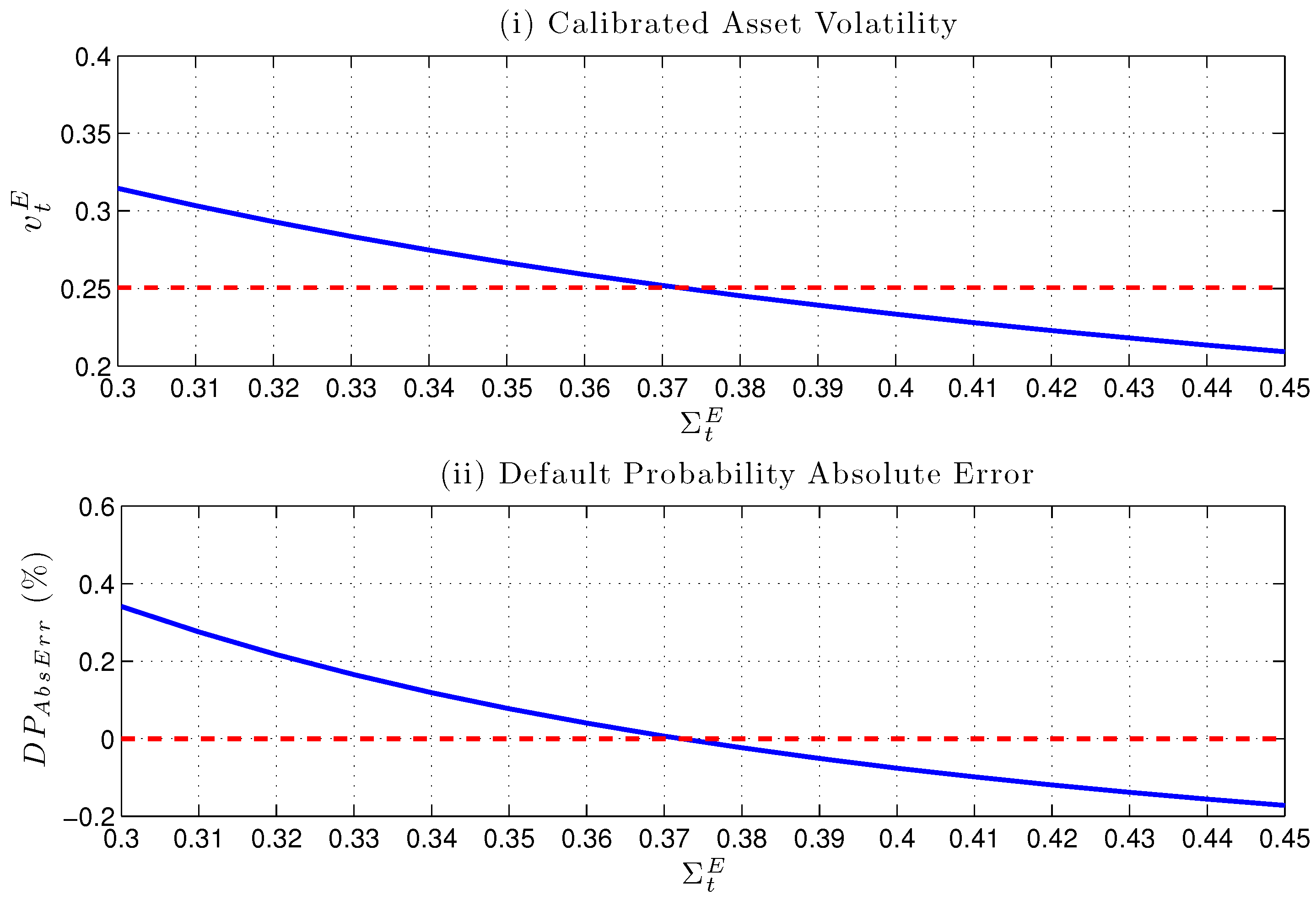
In order to understand the influence of alternative equity volatility estimators on both asset volatility calibration and default probability computation, we preliminarily show in Figure 4 the theoretical relationship between these quantities. The idea is to take as base case the pair of parameters ${\Sigma }_t^s=37.21\%,$$v_t=25.01\%$ and evaluate the impact of different equity volatility values ${\Sigma }_t^E\in [0.3,0.45]$ through our calibration device on both calibrated asset volatility and default probability, as if ${\Sigma }_t^E$ was the equity volatility estimate obtained through the non-parametric estimator E. The theoretical dependence of the calibrated asset volatility $v_t^E$ and the default probability is shown in Figure 4 for the Bates model, but the qualitative behaviour is the same also for the Heston model: as we can see, the equity volatility estimate is a key variable determining both the calibration of asset volatility and the default probability. The impact on default probability is measured in terms of the absolute error defined as $D{P}_{AbsErr}:=DP\left({\Sigma }_t^E\right)-DP\left({\Sigma }_t^s\right)$. The calibrated asset volatility depicted in Subplot (i) is obtained by matching the 5-years default probability $P{D}_5=1.37\%$, then this value is used to compute the absolute error on the 3-years default probability reported in Subplot (ii). To generalize the outcome of the analysis, the relationship between calibrated asset volatility and equity volatility estimation is nonlinear (convex) monotonous decreasing: overestimating equity volatility generates an underestimation of the calibrated asset volatility. The same monotonous decreasing relation holds between ${\Sigma }_t^E$ and the absolute error $D{P}_{AbsErr}$, but the absolute magnitude of the error changes may depend on whether we are under-estimating or over-estimating ${\Sigma }_t^s$ and which time horizon we are considering. As a general feature, the influence of a non-correct equity volatility estimation can be not negligible. Thus, from a credit risk perspective, a robust equity volatility estimator is crucial to properly evaluate default probability at each maturity.

5.1. Equity Volatility Estimation with High-Frequency Data

We perform a Monte Carlo simulation by generating a sample of 1000 trading days and equispaced intra-day data at the frequency $h=1$ min (i.e., $n=1440$). Once the underlying asset value dynamics is generated by model (2), high-frequency equity prices are obtained through the no arbitrage method given by Equation (3). Market microstructure noise is considered, alternatively, for both cases described by Equations (6) and (7). The random shocks ${\eta }_j$ are i.i.d Gaussian random variables with zero mean and standard deviation equal to $1.4$ times the log-equity return standard deviation. We set $\alpha =0.5$ in the dependent noise case (7).

In the case of Bates model, the generated dataset is cleaned for jumps according to the jump removal procedure sketched in Section 3. This procedure allows to eliminate around 7.5%–10% of days from our sample. Nevertheless, some days in the cleaned sample may still exhibit small jumps that can affect volatility estimation. In particular, days in our sample can present different statistical autocorrelation structures. 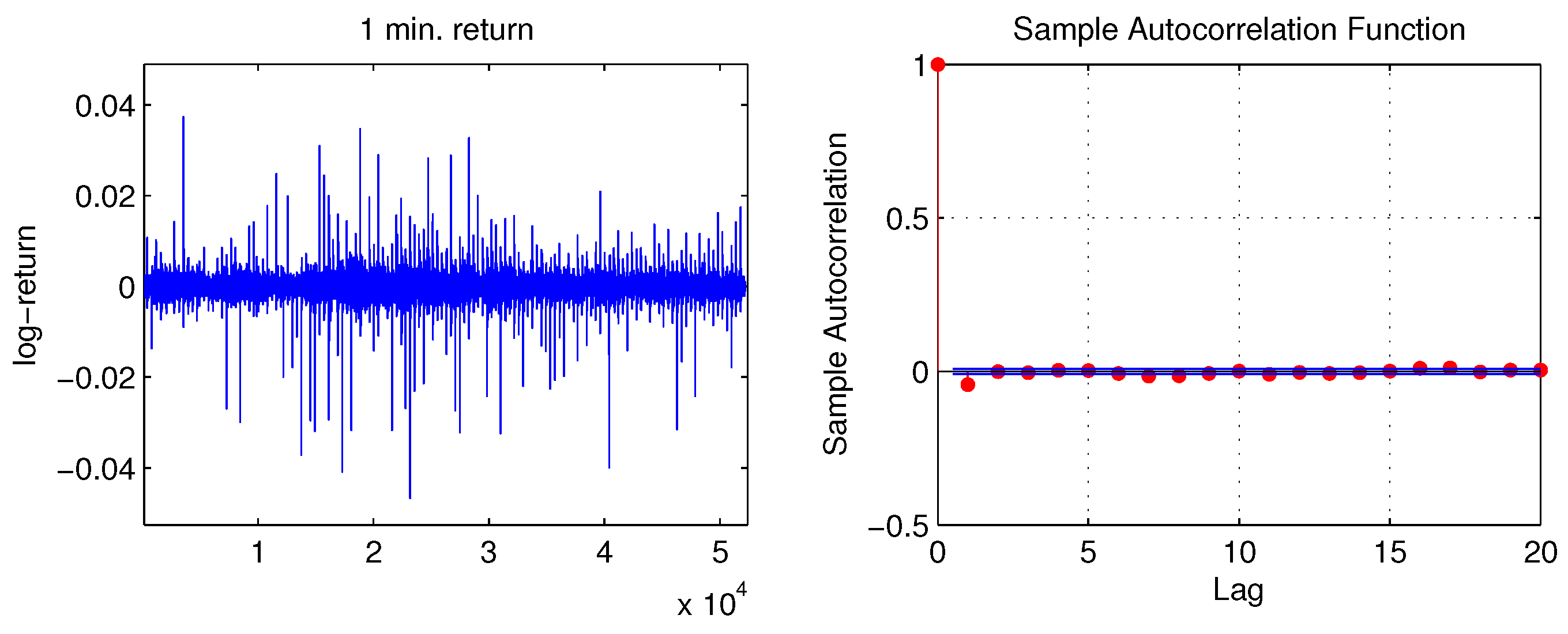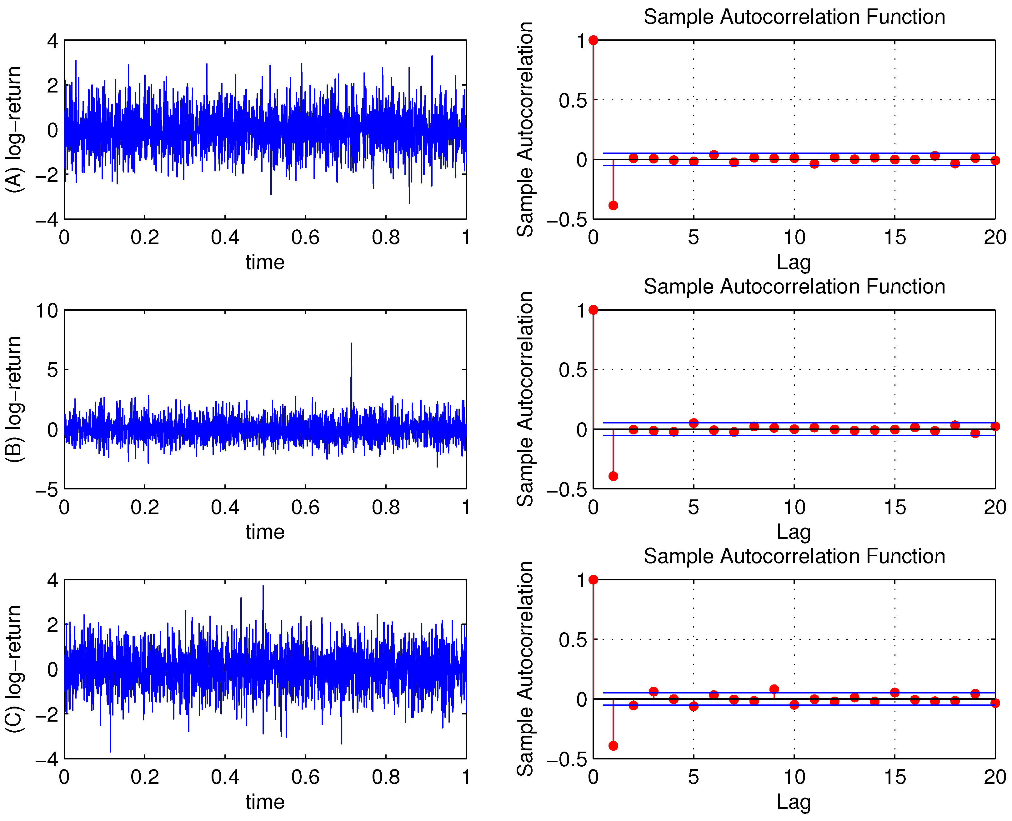Figure 5 shows the intraday log-returns, normalized to have mean zero and standard deviation one, for the model with Gaussian uncorrelated noise. Panel (A) refers to a day with no jumps and first order autocorrelation structure; panel (B) shows a big spike corresponding to a jump in the equity log-price process, still retaining a first order autocorrelation structure; (C) refers to a day with no jumps and autocorrelation at lags 3, 5, 9 and 15.

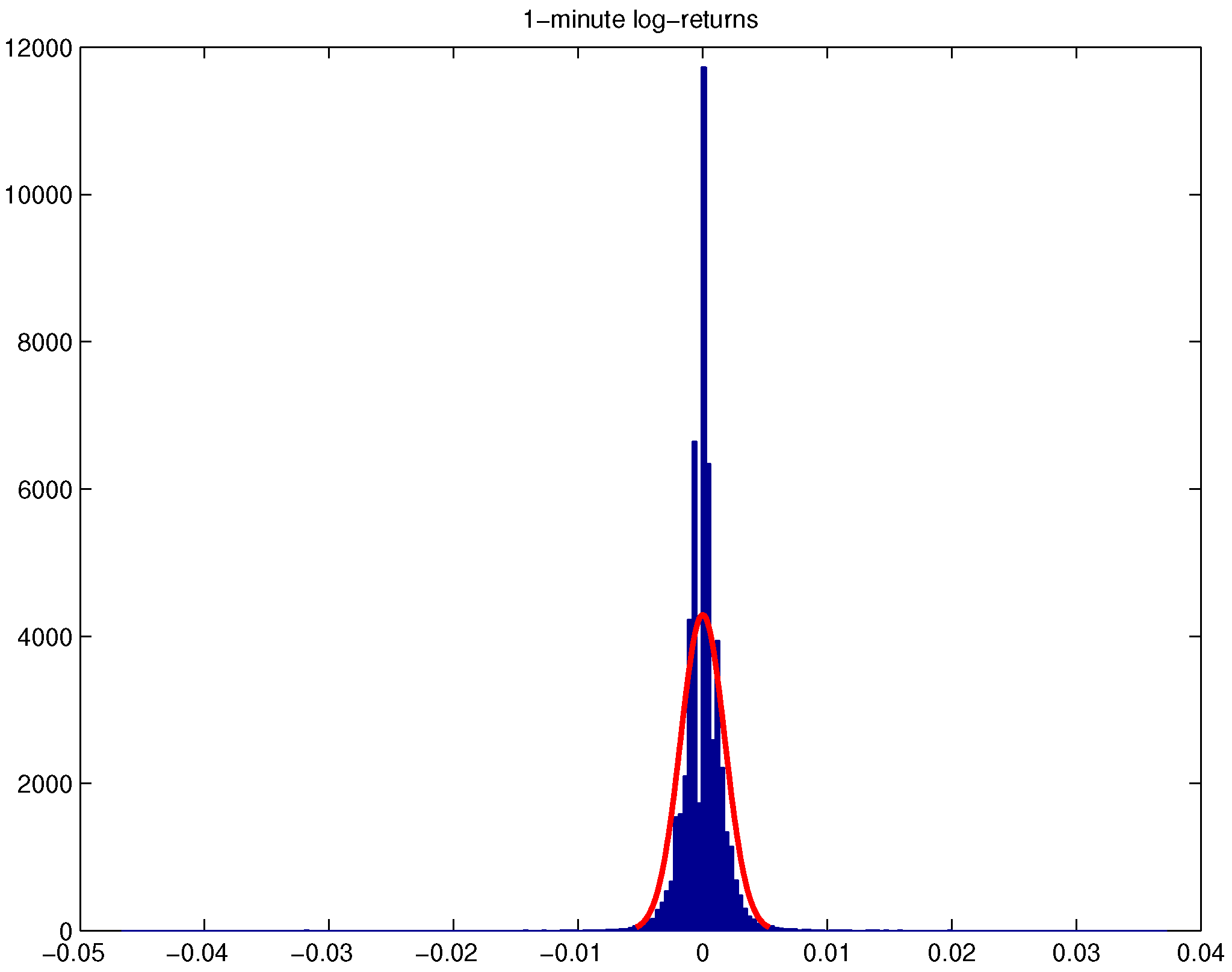
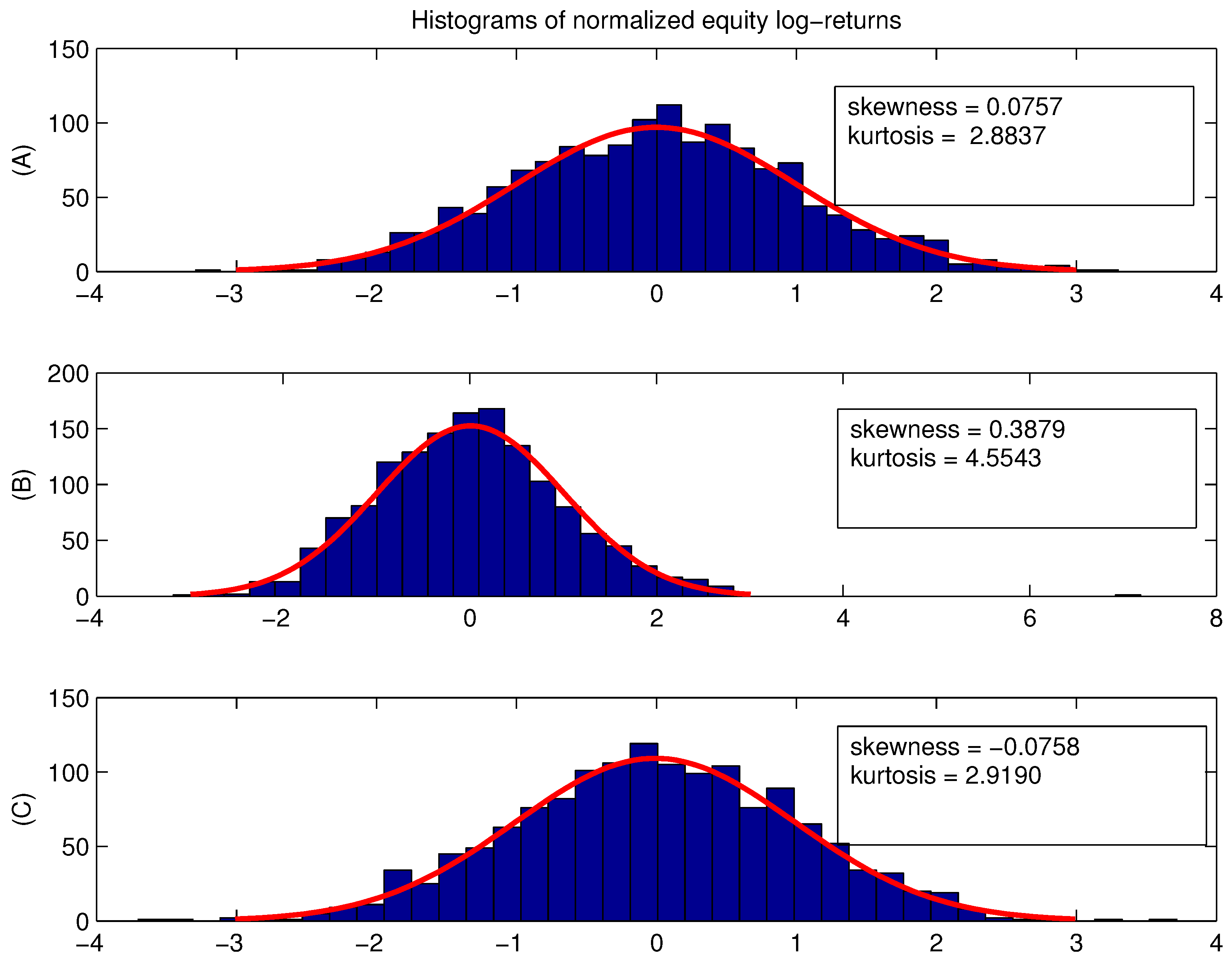
Next we plot the histograms of the intraday returns of equity log-prices. Figure 6 displays the histogram along with the standard normal density function, which is essentially confined within $(-3,3)$. Clearly, the histograms display a slightly high peak and asymmetric heavy tails. The distribution in case (B) is leptokurtic, i.e., more outlier-prone than the normal distribution. Moreover, skewness is positive, i.e., the data are spread out more to the right of the mean than to the left and the returns have heavier right tail.

Table 5. Heston model: performance of equity volatility estimators.

Heston		${\Sigma }_t^{\mathit{BV}}$	${\Sigma }_t^{\mathit{RV}}$	${\Sigma }_t^{\mathit{RVSS}}$	${\Sigma }_t^{\mathit{TS}}$	${\Sigma }_t^{\mathit{HL}}$	${\Sigma }_t^K$	${\Sigma }_t^{\mathit{PA}}$	${\Sigma }_t^F$
(a)	MSE	1.79 × 10${}^{-3}$	1.31 × 10${}^{-2}$	1.65 × 10${}^{-3}$	3.43 × 10${}^{-4}$	1.05 × 10${}^{-3}$	4.37 × 10${}^{-4}$	5.10 × 10${}^{-4}$	5.09 × 10${}^{-4}$
	BIAS	2.35 × 10${}^{-2}$	1.13 × 10${}^{-1}$	2.62 × 10${}^{-2}$	–1.47 × 10${}^{-3}$	–9.48 × 10${}^{-4}$	−7.69 × 10${}^{-4}$	–4.77 × 10${}^{-3}$	4.57 × 10${}^{-3}$
(b)	MSE	2.42 × 10${}^{-3}$	2.28 × 10${}^{-2}$	2.30 × 10${}^{-3}$	3.58 × 10${}^{-4}$	1.66 × 10${}^{-3}$	4.64 × 10${}^{-4}$	5.05 × 10${}^{-4}$	5.71 × 10${}^{-4}$
	BIAS	2.84 × 10${}^{-2}$	1.48 × 10${}^{-1}$	3.21 × 10${}^{-2}$	−7.66 × 10${}^{-4}$	5.10 × 10${}^{-4}$	–3.72 × 10${}^{-4}$	−4.20 × 10${}^{-3}$	6.06 × 10${}^{-3}$

Note: The table shows mean squared error (MSE) and BIAS for different equity volatility estimators. Panel (a) refers to the trading noise given in Equation (6), panel (b) to Equation (7), with $\alpha =0.5$. The underlying dynamics follows Heston [17] model.

and

Table 6. Bates model: performance of equity volatility estimators.

Bates		${\Sigma }_t^{\mathit{BV}}$	${\Sigma }_t^{\mathit{RV}}$	${\Sigma }_t^{\mathit{RVSS}}$	${\Sigma }_t^{\mathit{TS}}$	${\Sigma }_t^{\mathit{HL}}$	${\Sigma }_t^K$	${\Sigma }_t^{\mathit{PA}}$	${\Sigma }_t^F$
(a)	MSE	2.77 × 10${}^{-3}$	1.63 × 10${}^{-2}$	2.36 × 10${}^{-3}$	4.69 × 10${}^{-4}$	1.23 × 10${}^{-3}$	5.44 × 10${}^{-4}$	5.50 × 10${}^{-4}$	6.75 × 10${}^{-4}$
	BIAS	3.16 × 10${}^{-2}$	1.24 × 10${}^{-1}$	3.19 × 10${}^{-2}$	7.18 × 10${}^{-4}$	2.08 × 10${}^{-3}$	2.10 × 10${}^{-3}$	-2.45 × 10${}^{-3}$	8.40 × 10${}^{-3}$
(b)	MSE	3.36 × 10${}^{-3}$	2.78 × 10${}^{-2}$	3.12 × 10${}^{-3}$	6.37 × 10${}^{-4}$	1.88 × 10${}^{-3}$	7.18 × 10${}^{-4}$	7.51 × 10${}^{-4}$	8.91 × 10${}^{-4}$
	BIAS	3.40 × 10${}^{-2}$	1.63 × 10${}^{-1}$	3.71 × 10${}^{-2}$	–6.38 × 10${}^{-4}$	1.54 × 10${}^{-3}$	2.43 × 10${}^{-3}$	–1.65 × 10${}^{-3}$	1.03 × 10${}^{-2}$

Note: The table shows mean squared error (MSE) and BIAS for different equity volatility estimators. Panel (a) refers to the trading noise given in Equation (6), panel (b) to Equation (7), with $\alpha =0.5$. The underlying dynamics follows [18] model.

present numerical evidence for each equity volatility estimator introduced in Section 2 and used in our comparison when (a) trading noise is independent of intra-day equity log-returns and (b) trading noise is correlated with intra-day equity log-returns, respectively; both Heston [17] and Bates [18] dynamics are considered. All the estimators are applied on the equity log-price series after jump removal. The only exception is for the jump-robust Bipower Variation which is applied to the original dataset including jumps after optimal sparse sampling.

Table 5 and Table 6 list the mean squared error (MSE) and bias (BIAS) achieved by the different non-parametric equity volatility estimators. ${\Sigma }_t^{RV}$ represents the sparse sampled Realized Volatility estimator based on 5-min returns, while ${\Sigma }_t^{RVSS}$ refers to the sparse sampled Realized Volatility estimator where the sampling frequency is optimized in order to filter the microstructure effects, as explained in Section 2. Our results strongly confirm well known stylized facts documented by the econometric literature and highlighted by [24]: ${\Sigma }_t^{RV}$ estimates are strongly affected by noise and sparse sampling can only moderately provide efficient estimates. The 5-min Realized Volatility estimator has the worst performance in terms of both MSE and BIAS among all estimators for Heston and Bates settings, with a MSE of order $e-02$ and BIAS of order $e-01$. This performance can be even worst when considering the 1-min Realized Volatility estimator: results are not reported in the table, but equity volatility estimates are completely swamped by trading noise in such a case. The performance of the Bipower Variation estimator ${\Sigma }_t^{BV}$ for equity volatility is comparable to the one obtained through the Realized Volatility estimator based on sparse sampling ${\Sigma }_t^{RVSS}$. This is particularly relevant in the Bates model simulation of Table 6. In fact, jumps have been removed from our samples using the procedure sketched in Section 2. Although some of the jumps may still be present after jump removal, this procedure seems to be effective in eliminating the most relevant jumps.

As an alternative to sparse sampling, the first order correction of ${\Sigma }_t^{HL}$ can reduce the bias due to the spurious first order autocorrelation in equity returns introduced by the trading noise: overall, this estimator performs much better than ${\Sigma }_t^{RVSS}$ in both models and for both assumptions on the trading noise. However, the BIAS reduction is more effective in the Heston model.

The best results in terms of MSE are obtained when considering the set of estimators specifically designed to handle microstructure effects, i.e., ${\Sigma }_t^{TS}$, ${\Sigma }_t^K$, ${\Sigma }_t^{PA}$ and ${\Sigma }_t^F$.

If we want to try to rank the estimators according to the noise provision, we can state that both the Two-Scale ${\Sigma }_t^{TS}$ and the Kernel estimators ${\Sigma }_t^K$ have the best performance in Heston setting, with ${\Sigma }_t^K$ having a smaller BIAS. The performance of the pre-averaging estimator ${\Sigma }_t^{PA}$ and the Fourier estimator ${\Sigma }_t^F$ are comparable in both models.

5.2. Asset Volatility Calibration

This section analyzes how the choice of different volatility estimators affects the calibration of the underlying asset volatility. In order to study the influence of different equity volatility estimators on the default probability predicted by Merton model (see [1]), we proceed by developing the following calibration exercise for the underlying asset volatility. For each equity volatility estimator, generically denoted by E, and each day t in our sample, we find the corresponding daily asset volatility estimate ${\widehat{v_t}}^E$ by matching the 5-years default probability coming from our equity volatility estimate ${\Sigma }_t^E$ with the one evaluated through the model using the parameter values of Table 4. This is done for each day in the sample. In this calibration exercise we act as if we did not know the asset values to mimic the real-life estimation situation and we conduct inference only based on observable quantities such as measurable equity volatility and the 5-years default probabilities. Default probabilities are computed, for any maturity, according to Equation (5). In order to avoid arbitrage opportunities, following [9], we consider as key assumption that all securities written on the underlying firm value $A_t$ must have the same Sharpe ratio, see (8) (cfr. Equation (6) in [1]). This consideration enables us to express the instantaneous asset return μ as a function of the unknown asset volatility, given each equity volatility estimate ${\Sigma }_t^E$, and then to solve Equation (5) for the 5-years default probability with respect to the asset volatility, to obtain the corresponding asset volatility estimate ${\widehat{v_t}}^E$. Once asset volatility is known, we can compute default probabilities for any other maturity according to Equation (5).

Table 7. Heston model: calibrated asset volatility.

Heston
		Mean	Median	10 perc.	90 perc.	Min	Max	Std Dev.
(a)	${\widehat{v_t}}^{BV}$	0.2082	0.2056	0.1833	0.2350	0.1614	0.2960	0.0205
	${\widehat{v_t}}^{RV}$	0.1704	0.1699	0.1599	0.1815	0.1453	0.2027	0.0085
	${\widehat{v_t}}^{RVSS}$	0.2063	0.2045	0.1838	0.2308	0.1583	0.2922	0.0182
	${\widehat{v_t}}^{TS}$	0.2214	0.2202	0.2035	0.2410	0.1831	0.2718	0.0151
	${\widehat{v_t}}^{HL}$	0.2229	0.2195	0.1950	0.2554	0.1764	0.3385	0.0243
	${\widehat{v_t}}^K$	0.2210	0.2202	0.2021	0.2406	0.1802	0.2736	0.0155
	${\widehat{v_t}}^{PA}$	0.2238	0.2228	0.2029	0.2453	0.1802	0.2774	0.0166
	${\widehat{v_t}}^F$	0.2178	0.2169	0.1984	0.2375	0.1776	0.2684	0.0156
	${\widehat{v_t}}^{BV}/v_t$	0.9617	0.9498	0.8464	1.0853	0.7454	1.3673	0.0948
	${\widehat{v_t}}^{RV}/v_t$	0.7870	0.7845	0.7387	0.8383	0.6709	0.9364	0.0392
	${\widehat{v_t}}^{RVSS}/v_t$	0.9528	0.9448	0.8489	1.0659	0.7310	1.3495	0.0840
	${\widehat{v_t}}^{TS}/v_t$	1.0226	1.0172	0.9400	1.1134	0.8456	1.2554	0.0696
	${\widehat{v_t}}^{HL}/v_t$	1.0297	1.0140	0.9005	1.1796	0.8149	1.5637	0.1123
	${\widehat{v_t}}^K/v_t$	1.0210	1.0169	0.9335	1.1113	0.8326	1.2637	0.0714
	${\widehat{v_t}}^{PA}/v_t$	1.0337	1.0290	0.9371	1.1329	0.8326	1.2815	0.0766
	${\widehat{v_t}}^F/v_t$	1.0061	1.0018	0.9164	1.0970	0.8203	1.2396	0.0722
(b)	${\widehat{v_t}}^{BV}$	0.2062	0.2040	0.1791	0.2368	0.1485	0.2902	0.0227
	${\widehat{v_t}}^{RV}$	0.1602	0.1600	0.1503	0.1705	0.1361	0.1846	0.0079
	${\widehat{v_t}}^{RVSS}$	0.2036	0.2023	0.1802	0.2300	0.1571	0.2942	0.0196
	${\widehat{v_t}}^{TS}$	0.2209	0.2193	0.2021	0.2413	0.1781	0.2777	0.0153
	${\widehat{v_t}}^{HL}$	0.2234	0.2180	0.1909	0.2637	0.1658	0.3779	0.0309
	${\widehat{v_t}}^K$	0.2209	0.2193	0.2007	0.2429	0.1782	0.2942	0.0164
	${\widehat{v_t}}^{PA}$	0.2235	0.2226	0.2020	0.2462	0.1791	0.2959	0.0172
	${\widehat{v_t}}^F$	0.2170	0.2156	0.1967	0.2397	0.1760	0.2849	0.0165
	${\widehat{v_t}}^{BV}/v_t$	0.9391	0.9282	0.8200	1.0757	0.7079	1.2751	0.0984
	${\widehat{v_t}}^{RV}/v_t$	0.7298	0.7296	0.6947	0.7635	0.6308	0.8285	0.0273
	${\widehat{v_t}}^{RVSS}/v_t$	0.9276	0.9216	0.8227	1.0357	0.7396	1.3023	0.0838
	${\widehat{v_t}}^{TS}/v_t$	1.0061	1.0023	0.9348	1.0789	0.8673	1.2023	0.0553
	${\widehat{v_t}}^{HL}/v_t$	1.0176	0.9911	0.8757	1.1951	0.7826	1.8007	0.1353
	${\widehat{v_t}}^K/v_t$	1.0060	1.0006	0.9283	1.0914	0.8423	1.2411	0.0627
	${\widehat{v_t}}^{PA}/v_t$	1.0176	1.0121	0.9359	1.1062	0.8570	1.2606	0.0662
	${\widehat{v_t}}^F/v_t$	0.9883	0.9834	0.9103	1.0734	0.8388	1.2148	0.0642

Note: The table shows descriptive statistics of calibrated asset volatility for different equity volatility estimators. Results are based on 1000 daily Monte Carlo simulations. Panel (a) refers to the trading noise given in Equation (6), panel (b) to Equation (7), with $\alpha =0.5$.

shows descriptive statistics of calibrated asset volatility for the Heston model,

Table 8. Bates model: calibrated asset volatility.

Bates
		Mean	Median	10 perc.	90 perc.	Min	Max	Std Dev.
(a)	${\widehat{v_t}}^{BV}$	0.2526	0.2497	0.2076	0.3012	0.1558	0.3792	0.0381
	${\widehat{v_t}}^{RV}$	0.2042	0.2038	0.1893	0.2211	0.1597	0.2502	0.0125
	${\widehat{v_t}}^{RVSS}$	0.2502	0.2477	0.2202	0.2839	0.1826	0.3503	0.0254
	${\widehat{v_t}}^{TS}$	0.2703	0.2701	0.2459	0.2962	0.2018	0.3360	0.0203
	${\widehat{v_t}}^{HL}$	0.2714	0.2673	0.2361	0.3140	0.1857	0.3739	0.0304
	${\widehat{v_t}}^K$	0.2694	0.2673	0.2444	0.2979	0.2007	0.3411	0.0215
	${\widehat{v_t}}^{PA}$	0.2730	0.2710	0.2470	0.3018	0.2019	0.3498	0.0223
	${\widehat{v_t}}^F$	0.2648	0.2624	0.2396	0.2928	0.1980	0.3340	0.0215
	${\widehat{v_t}}^{BV}/v_t$	0.9391	0.9241	0.7605	1.1260	0.5392	1.4802	0.1501
	${\widehat{v_t}}^{RV}/v_t$	0.7579	0.7573	0.7169	0.8034	0.5801	0.8881	0.0355
	${\widehat{v_t}}^{RVSS}/v_t$	0.9283	0.9208	0.8262	1.0473	0.6491	1.2119	0.0860
	${\widehat{v_t}}^{TS}/v_t$	1.0027	1.0020	0.9312	1.0833	0.7840	1.2004	0.0600
	${\widehat{v_t}}^{HL}/v_t$	1.0068	0.9931	0.8884	1.1467	0.7437	1.4164	0.1036
	${\widehat{v_t}}^K/v_t$	0.9994	0.9931	0.9222	1.0891	0.7794	1.2373	0.0659
	${\widehat{v_t}}^{PA}/v_t$	1.0127	1.0071	0.9315	1.1073	0.7852	1.2410	0.0684
	${\widehat{v_t}}^F/v_t$	0.9825	0.9771	0.9027	1.0745	0.7727	1.2113	0.0668
(b)	${\widehat{v_t}}^{BV}$	0.2521	0.2485	0.2067	0.3055	0.1616	0.3794	0.0387
	${\widehat{v_t}}^{RV}$	0.1909	0.1909	0.1787	0.2043	0.1511	0.2252	0.0106
	${\widehat{v_t}}^{RVSS}$	0.2474	0.2450	0.2160	0.2825	0.1727	0.3627	0.0270
	${\widehat{v_t}}^{TS}$	0.2712	0.2694	0.2451	0.2990	0.2019	0.3480	0.0212
	${\widehat{v_t}}^{HL}$	0.2726	0.2682	0.2318	0.3228	0.1847	0.3797	0.0347
	${\widehat{v_t}}^K$	0.2692	0.2686	0.2424	0.2978	0.1918	0.3456	0.0225
	${\widehat{v_t}}^{PA}$	0.2726	0.2721	0.2446	0.3029	0.1921	0.3568	0.0238
	${\widehat{v_t}}^F$	0.2636	0.2633	0.2368	0.2924	0.1880	0.3481	0.0224
	${\widehat{v_t}}^{BV}/v_t$	0.9378	0.9222	0.7570	1.1482	0.5435	1.4866	0.1514
	${\widehat{v_t}}^{RV}/v_t$	0.7089	0.7096	0.6710	0.7494	0.5672	0.8206	0.0322
	${\widehat{v_t}}^{RVSS}/v_t$	0.9187	0.9101	0.8112	1.0389	0.6286	1.4060	0.0940
	${\widehat{v_t}}^{TS}/v_t$	1.0070	1.0024	0.9246	1.0972	0.7306	1.2813	0.0700
	${\widehat{v_t}}^{HL}/v_t$	1.0129	0.9981	0.8711	1.1864	0.6801	1.4773	0.1275
	${\widehat{v_t}}^K/v_t$	0.9997	0.9971	0.9115	1.0918	0.6901	1.2540	0.0724
	${\widehat{v_t}}^{PA}/v_t$	1.0120	1.0086	0.9222	1.1073	0.6911	1.2946	0.0766
	${\widehat{v_t}}^F/v_t$	0.9786	0.9767	0.8952	1.0681	0.6766	1.2632	0.0719

Note: The table shows descriptive statistics of calibrated asset volatility for different equity volatility estimators. Results are based on a sample of 934 days in case (a) and 901 days in case (b) for our Monte Carlo simulations (due to jumps removal). Panel (a) refers to the trading noise given in Equation (6), panel (b) to Equation (7), with $\alpha =0.5$.

contains statistics for the Bates case. We report results obtained by matching 5-years default probabilities for each equity volatility estimator E. Panel (a) of both tables refers to a trading noise of the form (6); panel (b) refers to results obtained for a trading noise of the form (7). The set of equity volatility estimators represented by Two-scale, Kernel, Fourier and Pre-Average estimators provides the most accurate estimation of the resulting calibrated daily asset volatility for Heston case, showing the smallest standard deviation. The same behavior is confirmed by results under Bates setting in Table 8. These results are confirmed by statistics for the ratio ${\widehat{v_t}}^E/v_t$, where the variable $v_t$ is the underlying asset volatility calibrated by considering the model daily equity volatility ${\Sigma }_t^s$ on each day t in the Monte Carlo sample. In particular, it is evident how the high-frequency Realized Volatility procedure largely underestimates the underlying asset volatility: ${\widehat{v_t}}^{RV}/v_t$ is strongly biased due to microstructure effects, while the optimized ${\widehat{v_t}}^{RVSS}$ is less biased, even if a slightly larger variance appears.

5.3. Default Probability Computation

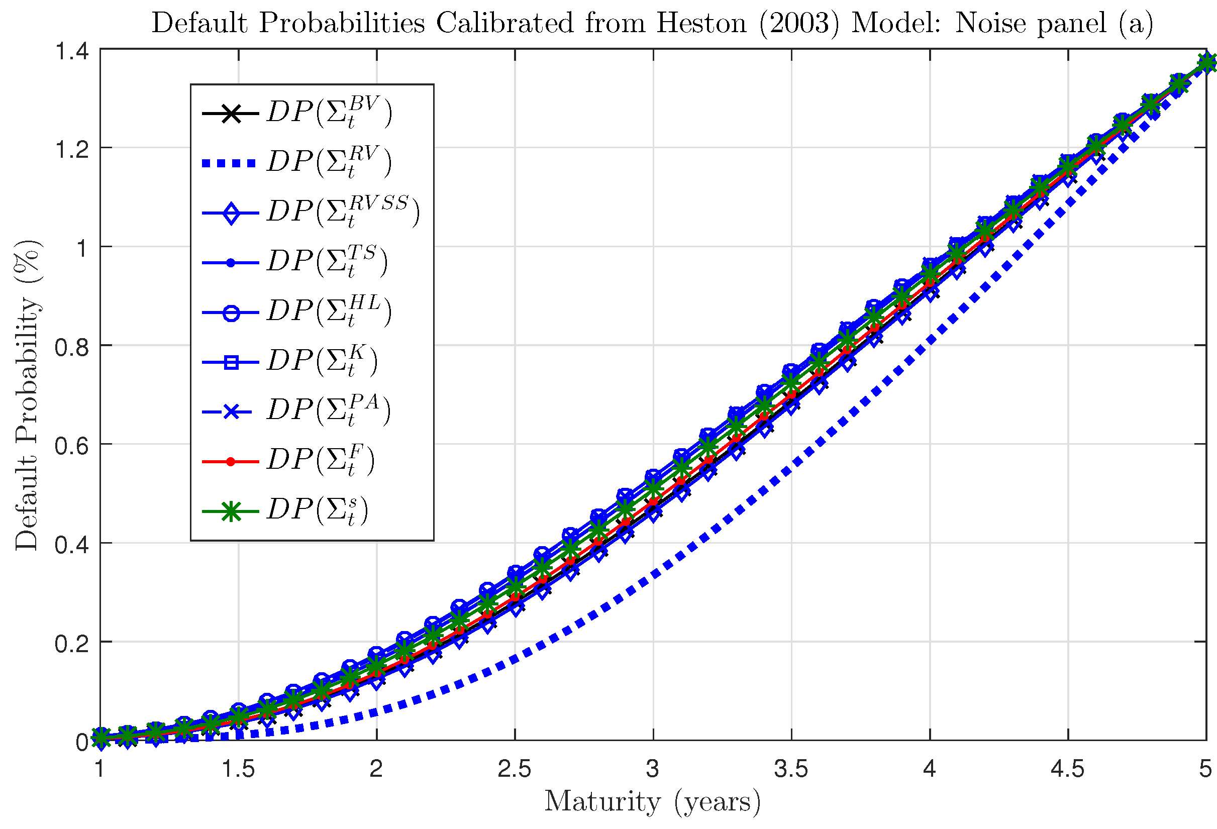
Once asset volatility is calibrated, we can turn to default probability computation. The average (over the daily Monte Carlo replications) default probabilities for different maturities obtained from alternative equity volatility estimation procedures are plotted in Figure 7 for Heston case, Gaussian noise. For each day in the sample and for each volatility estimator $E,$ we use the calibrated asset volatility ${\widehat{v_t}}^E$ in order to compute the default probabilities for any maturity (from 1 to 5 years) through Equation (5). The figure highlights how the Realized Volatility approach based on high frequency noisy data drastically underestimates default probabilities, thus sparse sampling becomes mandatory when equity data are affected by microstructure effects. On the whole, all the other procedures seem to provide sensible results and only a deeper analysis reveals differences among different specific estimators, as shown in

Table 9. Heston model: default probability relative error.

Heston		${\mathit{DP}}_{\mathit{Err}}^{\mathit{BV}}$	${\mathit{DP}}_{\mathit{Err}}^{\mathit{RV}}$	${\mathit{DP}}_{\mathit{Err}}^{\mathit{RVSS}}$	${\mathit{DP}}_{\mathit{Err}}^{\mathit{TS}}$	${\mathit{DP}}_{\mathit{Err}}^{\mathit{HL}}$	${\mathit{DP}}_{\mathit{Err}}^K$	${\mathit{DP}}_{\mathit{Err}}^{\mathit{PA}}$	${\mathit{DP}}_{\mathit{Err}}^F$
(a)	1 y	−13.3336	−92.8243	−28.5112	21.9938	78.9713	23.4477	42.2060	7.7918
	1.5 y	−17.5285	−78.4652	−24.5641	9.0594	26.2613	9.1401	18.3708	0.2651
	2 y	−14.7317	−62.4385	−18.8872	4.7895	12.3708	4.6020	10.1900	−1.1713
	2.5 y	−11.3451	−47.6616	−14.0002	2.8063	6.7021	2.5822	6.2117	−1.3314
	3 y	−8.2927	−34.8476	−10.0211	1.7067	3.8412	1.5118	3.9022	−1.1385
	3.5 y	−5.6774	−23.9395	−6.7715	1.0330	2.2124	0.8872	2.4191	−0.8426
	4 y	−3.4884	−14.7071	−4.1215	0.5700	1.1696	0.4737	1.3652	−0.5485
	4.5 y	−1.6097	−6.8180	−1.8894	0.2438	0.4832	0.1978	0.5945	−0.2621
(b)	1 y	−13.4191	−96.3065	−31.8708	20.9369	168.7090	25.5428	42.4058	6.8763
	1.5 y	−19.3928	−85.0507	−28.2278	8.3951	44.9036	9.7227	18.0795	−0.8700
	2 y	−16.6626	−69.9185	−21.9503	4.3225	19.1746	4.8187	9.9133	−2.1040
	2.5 y	−12.9684	−54.5511	−16.3767	2.4793	9.7422	2.6783	6.0040	−2.0250
	3 y	−9.5387	−40.4839	−11.7690	1.4819	5.3111	1.5581	3.7556	−1.6324
	3.5 y	−6.5555	−28.1046	−7.9772	0.8845	2.9280	0.9107	2.3219	−1.1722
	4 y	−4.0377	−17.3914	−4.8619	0.4814	1.4919	0.4843	1.3077	−0.7493
	4.5 y	−1.8674	−8.1086	−2.2329	0.2037	0.5952	0.2015	0.5683	−0.3538

Note: The table shows default probability mean relative error given in Equation (9) for maturities from 1 to 4.5 years. Results are based on 1000 daily Monte Carlo simulations using different equity volatility estimators. Default probability relative errors are in percentage (%). The simulation is based on equi-spaced intra-day data generated on a 1-min frequency. Panel (a) refers to a trading noise defined by Equation (6), panel (b) to Equation (7).

and

Table 10. Bates model: default probability relative error.

Bates		${\mathit{DP}}_{\mathit{Err}}^{\mathit{BV}}$	${\mathit{DP}}_{\mathit{Err}}^{\mathit{RV}}$	${\mathit{DP}}_{\mathit{Err}}^{\mathit{RVSS}}$	${\mathit{DP}}_{\mathit{Err}}^{\mathit{TS}}$	${\mathit{DP}}_{\mathit{Err}}^{\mathit{HL}}$	${\mathit{DP}}_{\mathit{Err}}^K$	${\mathit{DP}}_{\mathit{Err}}^{\mathit{PA}}$	${\mathit{DP}}_{\mathit{Err}}^F$
(a)	1 y	14.4309	−87.1895	−29.9293	11.2133	36.5447	10.6474	22.8589	−2.1273
	1.5 y	−6.3833	−75.8094	−25.6593	5.0568	15.0133	4.1198	11.6211	−4.3575
	2 y	−10.3506	−62.5783	−20.5019	2.6651	7.5550	1.8140	6.9034	−4.1742
	2.5 y	−10.1010	−49.6830	−15.8434	1.5097	4.1438	0.8191	4.3846	−3.4849
	3 y	−8.4835	−37.7336	−11.7809	0.8810	2.3454	0.3568	2.8397	−2.6973
	3.5 y	−6.4324	−26.8797	−8.2676	0.4938	1.2813	0.1194	1.7782	−1.9495
	4 y	−4.2495	−17.0514	−5.1743	0.2556	0.6447	0.0189	1.0198	−1.2420
	4.5 y	−2.0866	−8.1234	−2.4413	0.1009	0.2468	−0.0116	0.4469	−0.5943
(b)	1 y	13.4257	−91.9420	−31.6169	18.4987	59.6240	13.0964	25.4460	−3.3672
	1.5 y	−6.7622	−82.7271	−28.0554	8.7867	24.5731	5.1571	12.4494	−5.5782
	2 y	−10.6074	−70.1849	−22.7147	4.8896	12.5041	2.3203	7.1783	−5.2046
	2.5 y	−10.3035	−56.8420	−17.6859	2.9221	6.9522	1.0776	4.4463	−4.3048
	3 y	−8.6408	−43.8048	−13.2162	1.7902	3.9822	0.4853	2.8177	−3.3196
	3.5 y	−6.5510	−31.5429	−9.3084	1.0624	2.2163	0.1803	1.7301	−2.3910
	4 y	−4.3266	−20.1699	−5.8425	0.5798	1.1333	0.0436	0.9752	−1.5208
	4.5 y	−2.1247	−9.6830	−2.7621	0.2422	0.4423	−0.0050	0.4206	−0.7267

Note: The table shows default probability mean relative error given in Equation (9) for maturities from 1 to 4.5 years. Due to jumps removal, results are based on a sample of 934 days in case (a) and 901 days in case (b) for our Monte Carlo simulations using different equity volatility estimators. Default probability relative errors are in percentage (%). The simulation is based on equispaced intra-day data generated on a 1-min frequency. Panel (a) refers to a trading noise being defined by Equation (6).

where relative errors are reported.

Comparing the performance of alternative equity volatility estimators on default probabilities is done for different maturities (from 1 to 5 years) through the mean relative error between the estimated default probability and the theoretical one. For each maturity, we consider the following measure>

$${DP}_{Err}^E:=\mathbb{E}\left[\frac{DP\left({\Sigma }_t^E\right)-DP\left({\Sigma }_t^s\right)}{DP\left({\Sigma }_t^s\right)}\right]·100,$$

(9)

where $DP\left({\Sigma }_t^E\right)$ is the default probability evaluated through Equation (5) when equity and asset volatility are estimated through a generic couple of estimators ${\Sigma }_t^E,{\widehat{v_t}}^E$; $DP\left({\Sigma }_t^s\right)$ is the corresponding theoretical default probability when equity and asset volatility are, respectively, ${\Sigma }_t^s$ and $v_t$ (model daily volatilities). Table 9 and Table 10 summarize the corresponding numerical results for both Heston and Bates cases, suggesting that the choice of the volatility estimator largely affects default probabilities.

Table 9 highlights that for the Heston model the smallest overall error on default probabilities is provided by the Fourier estimator, followed by the Two-Scales and the Kernel ones. For maturities greater than 2.5 years, even the ${\Sigma }_t^{HL}$ and Pre-Average estimators give good results. The optimally sampled Bipower Variation ${\Sigma }_t^{BV}$ provides results that are comparable with ${\Sigma }_t^{RVSS}$, underestimating the default risk. The classical 5-min Realized Volatility approach can severely underestimate risk, leading to an error of more than $90\%$ in absolute value for maturities before $1y$ and around 60%−70% in absolute value for maturities up to 2 years.

A similar ranking among estimators holds in Bates case, as reported in Table 10. While for maturities greater than 3 years the Kernel estimator has the best performance, i.e., the smallest average error on default probabilities, overall the Fourier estimator reveals to be the more stable one, with relative errors across all maturities being below $5.6\%$ in absolute value. Differently from the Fourier case, all other estimators show a peak in the default probability relative error for the $1y$ time horizon.

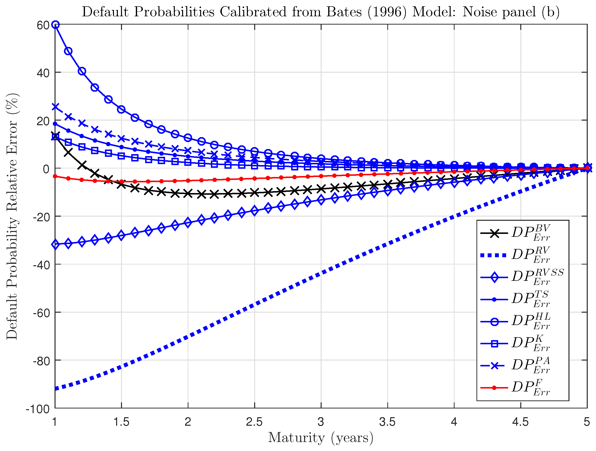
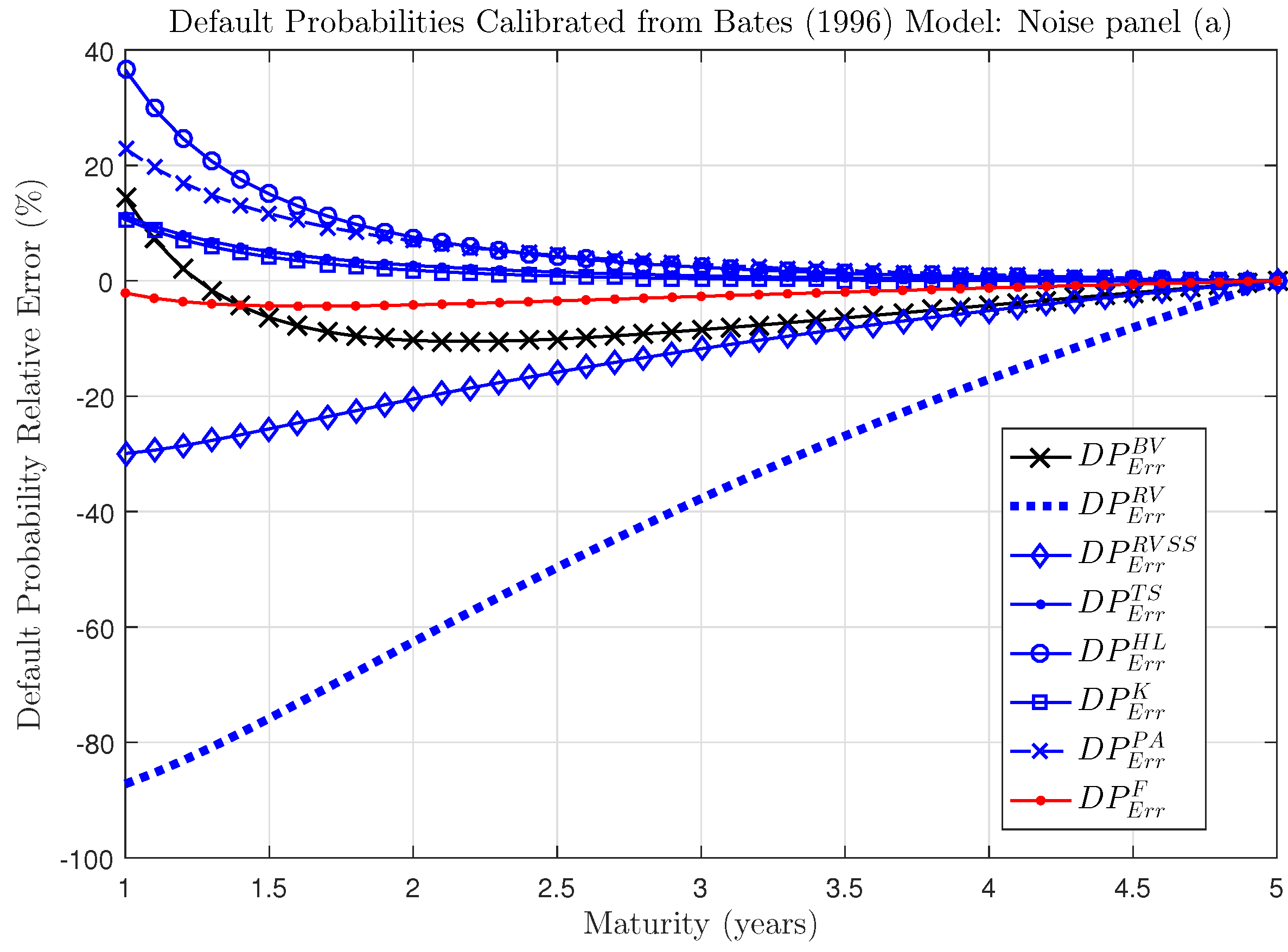
For a better visual insight, Figure 8 and Figure 9 show the mean relative error comparing different calibration procedures for Bates model, with, alternatively, Gaussian (a) and Correlated noise (b). A negative (positive) error reveals that the calibration procedure underestimates (overestimates) default probabilities. What emerges from the reported plots of default probability relative errors is that the Fourier estimator (red line in the Figures) is the most efficient, although it slightly underestimates default probabilities. This is due to the convexity of the non linear relationship between default probability error and asset volatility, as depicted in Figure 4 and discussed in Section 6. All the other estimators produce relative errors on default probabilities that are more inaccurate (and more volatile) as function of the maturity, reaching high absolute values for very short time horizons. The Realized Volatility estimator has a poor performance from 1y to 5y, always providing a significant underestimation of the default probability. This qualitative behavior reflects also results obtained for Heston setting, for both cases of Gaussian and Correlated trading noise and we omit them for brevity.

6. Sensitivity Analysis

In this Section we study the sensitivity of the asset volatility calibration and default probability estimation w.r.t. different values of the key parameters considered in our stochastic volatility setting: the correlation between volatility and returns (leverage effect) in Heston model, captured by parameter ρ, and the average percentage jump size in Bates model, captured by parameter ${\mu }_J$.

We consider as base case the setting described in the above analysis and define alternative sets of parameters. This is done by keeping unchanged the 5-years default probability $P{D}_{5y}=1.37\%$. The leverage effect is analyzed within Heston model in Section 6.1, while the sensitivity w.r.t. the jump parameter in Bates model is studied in Section 6.2. In both cases we consider a sample of 1000 days for the Monte Carlo simulation and a market microstructure effect described by a Correlated noise given in Equation (7). The simulations are based on equispaced intra-day data generated on a 1-min frequency. The analysis is conducted by exploring how the performance of different equity volatility estimators changes for different levels of the leverage effect and jump amplitude; then, the impact of equity volatility estimates on calibrated asset volatility and default probability is studied. From a credit risk perspective, this analysis is useful since it can suggest which equity volatility estimator is more appropriate depending on the specificity of the real dataset. The base cases presented below are the same already discussed in the previous section.

6.1. Leverage Effect

In this subsection we develop a sensitivity analysis on Heston model by considering alternative values of the correlation parameter ρ which captures the leverage effect. The idea is to quantify the impact of this key variable on both asset volatility calibration and default probability estimation.

Table 11. Test cases.

Heston
ρ	$v_0$
$\rho =-30.00\%$	$v_0=20.92\%$
$\rho =-24.02\%$	$v_0=21.65\%$
$\rho =0.0$	$v_0=24.20\%$

Note: The table summarizes the values considered in the sensitivity analysis for three alternative test cases associated with a 5-years default probability $P{D}_{5y}=1.37\%$.

summarizes the results of this analysis: starting from the base case described in the previous section, we compare the results associated to a correlation $\rho =-24.02\%$ with those obtained (i) for a higher (in absolute value) negative correlation $\rho =-30\%$ and (ii) for the uncorrelated case $\rho =0$. As well documented in the econometric literature, the leverage effect is known to be negative in financial markets, that is why we consider $\rho =0$ as extreme scenario. The initial asset volatility considered is the one corresponding to a 5-years default probability $P{D}_{5y}=1.37\%$ (see Table 11).

Table 12. Heston model: leverage effect on equity volatility estimators.

Heston		${\Sigma }_t^{\mathit{BV}}$	${\Sigma }_t^{\mathit{RV}}$	${\Sigma }_t^{\mathit{RVSS}}$	${\Sigma }_t^{\mathit{TS}}$	${\Sigma }_t^{\mathit{HL}}$	${\Sigma }_t^K$	${\Sigma }_t^{\mathit{PA}}$	${\Sigma }_t^F$
$\rho =-30\%$
	MSE	2.25 ×${10}^{-3}$	2.18 ×${10}^{-2}$	2.04 ×${10}^{-3}$	3.53 ×${10}^{-4}$	1.45 ×${10}^{-3}$	4.23 ×${10}^{-4}$	4.65 ×${10}^{-4}$	5.28 ×${10}^{-4}$
	BIAS	2.57 ×${10}^{-2}$	1.46 ×${10}^{-1}$	2.92 ×${10}^{-2}$	−5.06 ×${10}^{-4}$	−7.05 ×${10}^{-4}$	−1.96 ×${10}^{-5}$	−4.01 ×${10}^{-3}$	5.84 ×${10}^{-3}$
$\rho =-24.02\%$
	MSE	2.42 ×${10}^{-3}$	2.28 ×${10}^{-2}$	2.30 ×${10}^{-3}$	3.58 ×${10}^{-4}$	1.66 ×${10}^{-3}$	4.64 ×${10}^{-4}$	5.05 ×${10}^{-4}$	5.71 ×${10}^{-4}$
	BIAS	2.84 ×${10}^{-2}$	1.48 ×${10}^{-1}$	3.21 ×${10}^{-2}$	−7.66 ×${10}^{-4}$	5.10 ×${10}^{-4}$	−3.72 ×${10}^{-4}$	−4.20 ×${10}^{-3}$	6.06 ×${10}^{-3}$
$\rho =0$
	MSE	2.86 ×${10}^{-3}$	2.70 ×${10}^{-2}$	2.64 ×${10}^{-3}$	4.95 ×${10}^{-4}$	2.11 ×${10}^{-3}$	4.93 ×${10}^{-4}$	5.52 ×${10}^{-4}$	6.25 ×${10}^{-4}$
	BIAS	3.03 ×${10}^{-2}$	1.62 ×${10}^{-1}$	3.50 ×${10}^{-2}$	−1.62 ×${10}^{-3}$	−1.24 ×${10}^{-3}$	−1.64 ×${10}^{-4}$	−4.61 ×${10}^{-3}$	6.55 ×${10}^{-3}$

Note: The table shows mean squared error (MSE) and BIAS for different equity volatility estimators. The panel refers to the trading noise given in Equation (7), with $\alpha =0.5$. Alternative values for the correlation ρ are considered, i.e., $\rho \in \{-30\%,-24.02\%,0\}$.

reports MSE and BIAS of each equity volatility estimator under different levels of ρ. The outcome of our analysis highlights that the performance of equity volatility estimators is not much affected by the leverage parameter. Changing parameter ρ does not seem to generate a strong and significant directional impact on MSE and BIAS of the considered equity volatility estimators. Nevertheless, Table 12 reveals that the volatility estimators improve slightly their performance in terms of MSE as the negative leverage effect increases in absolute value; the Two-Scales, Kernel, Pre-Average and Fourier estimators give the best performance in terms of MSE, with an order of magnitude of $e-04$ in all cases.

As highlighted by

Table 13. Heston model: leverage effect on calibrated asset volatility.

Heston
		Mean	Median	10 perc.	90 perc.	Min	Max	Std Dev.
$\rho =-30\%$
	${\widehat{v_t}}^{BV}/v_t$	0.9414	0.9287	0.8099	1.0820	0.7170	1.6830	0.1100
	${\widehat{v_t}}^{RV}/v_t$	0.7112	0.7105	0.6753	0.7481	0.6333	0.8161	0.0285
	${\widehat{v_t}}^{RVSS}/v_t$	0.9286	0.9186	0.8180	1.0401	0.7280	1.5650	0.0909
	${\widehat{v_t}}^{TS}/v_t$	1.0055	1.0029	0.9322	1.0815	0.8502	1.2804	0.0598
	${\widehat{v_t}}^{HL}/v_t$	1.0209	0.9977	0.8745	1.1864	0.7505	1.7650	0.1370
	${\widehat{v_t}}^K/v_t$	1.0048	0.9991	0.9250	1.0881	0.8296	1.2480	0.0651
	${\widehat{v_t}}^{PA}/v_t$	1.0180	1.0123	0.9322	1.1079	0.8298	1.2640	0.0689
	${\widehat{v_t}}^F/v_t$	0.9875	0.9822	0.9061	1.0758	0.7997	1.2254	0.0672
$\rho =-24.02\%$
	${\widehat{v_t}}^{BV}/v_t$	0.9391	0.9282	0.8200	1.0757	0.7079	1.2751	0.0984
	${\widehat{v_t}}^{RV}/v_t$	0.7298	0.7296	0.6947	0.7635	0.6308	0.8285	0.0273
	${\widehat{v_t}}^{RVSS}/v_t$	0.9276	0.9216	0.8227	1.0357	0.7396	1.3023	0.0838
	${\widehat{v_t}}^{TS}/v_t$	1.0061	1.0023	0.9348	1.0789	0.8673	1.2023	0.0553
	${\widehat{v_t}}^{HL}/v_t$	1.0176	0.9911	0.8757	1.1951	0.7826	1.8007	0.1353
	${\widehat{v_t}}^K/v_t$	1.0060	1.0006	0.9283	1.0914	0.8423	1.2411	0.0627
	${\widehat{v_t}}^{PA}/v_t$	1.0176	1.0121	0.9359	1.1062	0.8570	1.2606	0.0662
	${\widehat{v_t}}^F/v_t$	0.9883	0.9834	0.9103	1.0734	0.8388	1.2148	0.0642
$\rho =0$
	${\widehat{v_t}}^{BV}/v_t$	0.9518	0.9420	0.8545	1.0614	0.7486	1.2600	0.0809
	${\widehat{v_t}}^{RV}/v_t$	0.7775	0.7768	0.7496	0.8061	0.7093	0.8636	0.0218
	${\widehat{v_t}}^{RVSS}/v_t$	0.9403	0.9371	0.8598	1.0316	0.7810	1.1655	0.0653
	${\widehat{v_t}}^{TS}/v_t$	1.0075	1.0031	0.9481	1.0687	0.8798	1.2356	0.0497
	${\widehat{v_t}}^{HL}/v_t$	1.0201	0.9972	0.8981	1.1718	0.8000	1.5879	0.1145
	${\widehat{v_t}}^K/v_t$	1.0044	0.9992	0.9440	1.0689	0.8841	1.1871	0.0494
	${\widehat{v_t}}^{PA}/v_t$	1.0147	1.0121	0.9497	1.0812	0.8880	1.2185	0.0529
	${\widehat{v_t}}^F/v_t$	0.9905	0.9879	0.9284	1.0535	0.8628	1.1834	0.0509

Note: The table shows descriptive statistics of calibrated asset volatility for different equity volatility estimators. The panel refers to the trading noise given in Equation (7), with $\alpha =0.5$. Alternative values for the correlation ρ are considered, i.e., $\rho \in \{-30\%,-24.02\%,0\}$.

, the leverage effect impacts the underlying asset volatility calibration: increasing the correlation level enhances the variance of the calibrated asset volatility, as the last column of the table shows. The 5-min Realized volatility estimator worsens its performance when $\rho (<0)$ increases in absolute value, reaching an average of asset volatility ratio of $71\%$. The same happens for the Bipower variation estimator and the Realized volatility estimator with sparse sampling: $BV$ worsen its asset volatility mean ratio from $95.2\%$ to $94.1\%$ going from $\rho =0$ to $\rho =-30\%$, while the $RVSS$ estimator shows results from $94\%$ to $92.8\%$ in the corresponding case studies. Results are even worst if we consider the 1-min Realized Volatility estimator, completely swamped by trading noise, and reaching less than $40\%$ in terms of mean asset volatility ratio. We recall that results for the 1-min Realized Volatility estimator are not reported to have a more consistent benchmark with all other estimators. In terms of standard deviation, the performance of ${\Sigma }_t^{TS},{\Sigma }_t^{HL},{\Sigma }_t^K,{\Sigma }_t^{PA},{\Sigma }_t^F$ is comparable, going from $4.9\%$ to $6.8\%$ depending on the level of the leverage ratio.

Table 14. Heston model: leverage effect on default probability estimation.

Heston		${\mathit{DP}}_{\mathit{Err}}^{\mathit{BV}}$	${\mathit{DP}}_{\mathit{Err}}^{\mathit{RV}}$	${\mathit{DP}}_{\mathit{Err}}^{\mathit{RVSS}}$	${\mathit{DP}}_{\mathit{Err}}^{\mathit{TS}}$	${\mathit{DP}}_{\mathit{Err}}^{\mathit{HL}}$	${\mathit{DP}}_{\mathit{Err}}^K$	${\mathit{DP}}_{\mathit{Err}}^{\mathit{PA}}$	${\mathit{DP}}_{\mathit{Err}}^F$
$\rho =-30\%$
	1 y	4.7996	−96.9042	−23.7409	22.3603	164.5229	24.3275	42.8046	6.8151
	1.5 y	−14.3485	−86.5006	−25.6429	8.5531	45.9491	9.0604	18.3006	−0.9973
	2 y	−14.2628	−71.7115	−20.5832	4.2434	20.1667	4.3702	10.0212	−2.2244
	2.5 y	−11.6035	−56.2816	−15.5388	2.3587	10.4761	2.3651	6.0606	−2.1285
	3 y	−8.7107	−41.9399	−11.2325	1.3717	5.8261	1.3378	3.7860	−1.7152
	3.5 y	−6.0728	−29.2146	−7.6546	0.7914	3.2556	0.7570	2.3270	−1.2429
	4 y	−3.7607	−18.1143	−4.6681	0.4249	1.6958	0.3979	1.3155	−0.7859
	4.5 y	−1.7491	−8.4585	−2.1484	0.1761	0.6865	0.1617	0.5710	−0.3716
$\rho =-24.02\%$
	1 y	−13.4191	−96.3065	−31.8708	20.9369	168.7090	25.5428	42.4058	6.8763
	1.5 y	−19.3928	−85.0507	-28.2278	8.3951	44.9036	9.7227	18.0795	−0.8700
	2 y	−16.6626	-69.9185	-21.9503	4.3225	19.1746	4.8187	9.9133	−2.1040
	2.5 y	−12.9684	−54.5511	−16.3767	2.4793	9.7422	2.6783	6.0040	−2.0250
	3 y	−9.5387	−40.4839	−11.7690	1.4819	5.3111	1.5581	3.7556	−1.6324
	3.5 y	−6.5555	−28.1046	−7.9772	0.8845	2.9280	0.9107	2.3219	−1.1722
	4 y	−4.0377	−17.3914	−4.8619	0.4814	1.4919	0.4843	1.3077	−0.7493
	4.5 y	−1.8674	−8.1086	−2.2329	0.2037	0.5952	0.2015	0.5683	−0.3538
$\rho =0$
	1y	−15.5280	−94.5066	−34.7584	22.5433	132.9700	18.0097	33.3303	2.8602
	1.5y	−18.0677	−81.4410	−27.5159	9.4160	40.9134	7.1596	15.0375	−1.7585
	2y	−14.9654	−65.8099	−20.6777	5.0341	18.8418	3.6290	8.5020	−2.2432
	2.5y	−11.4706	−50.7851	−15.1741	2.9833	10.1242	2.0582	5.2617	−1.9516
	3y	−8.3639	−37.4239	−10.7986	1.8339	5.7829	1.2193	3.3458	−1.5084
	3.5y	−5.7269	−25.8687	−7.2810	1.1117	3.3050	0.7165	2.0835	−1.0672
	4y	−3.5034	−15.9461	−4.4069	0.6189	1.7562	0.3880	1.1869	−0.6675
	4.5y	−1.6112	−7.3986	−2.0128	0.2692	0.7288	0.1665	0.5234	−0.3087

Note: The table shows default probability mean relative error given in Equation (9) for maturities from 1 to 4.5 years. Results are based on a sample of 1000 days for our Monte Carlo simulations. Default probability relative errors are in percentage (%). The panel refers to the trading noise given in Equation (7), with $\alpha =0.5$. Alternative values for the correlation ρ are considered, i.e., $\rho \in \{-30\%,-24.02\%,0\}$.

reports the results for the default probability errors under the three alternative settings associated to different leverage effects: all estimators (except the Fourier one) perform better in the uncorrelated case and get worse as the negative leverage effect increases in absolute value. From a credit risk perspective, this sensitivity analysis suggests that when dealing with a sample characterized by a correlation parameter ρ close to zero, the Kernel estimator should be preferred in order to evaluate the default probability, by reaching PD errors lower than $1.2\%$ for $3y$ and lower than $0.16\%$ for $4.5y$ maturity. The ${\Sigma }_t^{TS},{\Sigma }_t^{HL},{\Sigma }_t^{PA},{\Sigma }_t^F$ also provide good estimated for maturities greater than $3.5y$; for shorter maturities, the smallest errors are obtained by the Fourier estimator with an error of $-1.75\%$ for 1.5y and a maximum of $2.8\%$ for the 1y time horizon, significantly lower than errors obtained for the same short term maturity with all other estimators. At the same time, the Two-Scale, Kernel and Fourier estimators represent the best choice for a sample of data characterized by a more realistic high negative leverage effect: here the extreme case considered is $\rho =-30\%$, and ${\Sigma }_t^{TS},{\Sigma }_t^K,{\Sigma }_t^F$ show a good performance. For $\rho =-30\%$, the Fourier estimator still has the smallest volatility of default probability errors if compared with the performance of all other estimators.

By looking at asset volatility and equity volatility estimation, we can observe what follows: the performance of the three noise-robust estimators ${\Sigma }_t^{TS},{\Sigma }_t^K,{\Sigma }_t^F$ is comparable, and in some cases the Two-Scale and Kernel estimators can even do better than the Fourier one. Nevertheless, in terms of default probability relative error, the Fourier estimator provides better results, in particular for short maturities. The intuition behind the observed behavior is linked to the convexity of the non-linear relationship between default probability error and underlying asset volatility, as depicted in Figure 4. As we can observe, the relationship between default probability error and equity volatility estimates is non-linear and flattening as the equity volatility estimate increases. The same applies for the relationship between asset volatility and equity volatility. While the Two-Scale and Kernel estimators bring to an average overestimation of the underlying asset volatility, the Fourier estimates reveals an overall underestimation of the asset volatility. As a consequence, Fourier results are associated to a slight underestimation of the default probability while the Two-Scale and Kernel estimators can bring to higher default probability overestimation. This effect is amplified for short maturities, since the target variable to calibrate is the 5-years default probability.

6.2. Average Jumps Size

This section compares the performance of alternative non-parametric estimators for different values of the average jump size, measuring their sensitivity to parameter ${\mu }_J$. The aim of this analysis is to study how alternative scenarios with a different jump amplitude can affect asset volatility calibration and default probability estimation inside a setting described by the Bates model.

Table 15. Test cases.

Bates
${\mu }_J$	$v_0$
${\mu }_J=3.35\%$	$v_0=25.04\%$
${\mu }_J=2.35\%$	$v_0=25.01\%$
${\mu }_J=1.35\%$	$v_0=24.94\%$

Note: The table summarizes the values considered in this sensitivity analysis for three alternative test cases associated with a 5-years default probability $P{D}_{5y}=1.37\%$.

summarizes the cases we consider in this analysis: starting from the base parameters associated to ${\mu }_J=2.35\%$ (as in the previous Section, Table 4), we consider two alternative cases: one with higher average jump size ${\mu }_J=3.35\%$, one with lower average jump amplitude ${\mu }_J=1.35\%$. The initial asset volatility considered in each case is the one associated to a 5-years default probability $P{D}_{5y}=1.37\%$ (see Table 15). Here we consider a sample of 1000 days for our Monte Carlo simulation and a Correlated trading noise as defined in Equation (7). The simulation is again based on equispaced intra-day data generated on a 1-min frequency.

Results for the equity volatility estimators are reported in

Table 16. Bates model: effect of average jumps size on equity volatility estimators.

Bates		${\Sigma }_t^{\mathit{BV}}$	${\Sigma }_t^{\mathit{RV}}$	${\Sigma }_t^{\mathit{RVSS}}$	${\Sigma }_t^{\mathit{TS}}$	${\Sigma }_t^{\mathit{HL}}$	${\Sigma }_t^K$	${\Sigma }_t^{\mathit{PA}}$	${\Sigma }_t^F$
${\mu }_J=3.35\%$
	MSE	3.55 ×${10}^{-3}$	2.80 ×${10}^{-2}$	2.94 ×${10}^{-3}$	6.29 ×${10}^{-4}$	1.84 ×${10}^{-3}$	6.23 ×${10}^{-4}$	6.70 ×${10}^{-4}$	7.61 ×${10}^{-4}$
	BIAS	3.36 ×${10}^{-2}$	1.64 ×${10}^{-1}$	3.50 ×${10}^{-2}$	2.58 ×${10}^{-4}$	2.12 ×${10}^{-3}$	5.23 ×${10}^{-4}$	−3.99 ×${10}^{-3}$	7.70 ×${10}^{-3}$
${\mu }_J=2.35\%$
	MSE	3.36 ×${10}^{-3}$	2.78 ×${10}^{-2}$	3.12 ×${10}^{-3}$	6.37 ×${10}^{-4}$	1.88 ×${10}^{-3}$	7.18 ×${10}^{-4}$	7.51 ×${10}^{-4}$	8.91 ×${10}^{-4}$
	BIAS	3.40 ×${10}^{-2}$	1.63 ×${10}^{-1}$	3.71 ×${10}^{-2}$	−6.38 ×${10}^{-4}$	1.54 ×${10}^{-3}$	2.43 ×${10}^{-3}$	−1.65 ×${10}^{-3}$	1.03 ×${10}^{-2}$
${\mu }_J=1.35\%$
	MSE	3.32 ×${10}^{-3}$	2.81 ×${10}^{-2}$	2.74 ×${10}^{-3}$	5.31 ×${10}^{-4}$	1.81 ×${10}^{-3}$	5.42 ×${10}^{-4}$	5.85 ×${10}^{-4}$	6.83 ×${10}^{-4}$
	BIAS	3.51 ×${10}^{-2}$	1.65 ×${10}^{-1}$	3.58 ×${10}^{-2}$	4.81 ×${10}^{-4}$	2.37 ×${10}^{-3}$	1.15 ×${10}^{-3}$	−3.10 ×${10}^{-3}$	8.59 ×${10}^{-3}$

Note: The table shows mean squared error (MSE) and BIAS for different equity volatility estimators. The panel refers to the trading noise given in Equation (7), with $\alpha =0.5$. Alternative values for the jump parameter ${\mu }_J$ are considered: ${\mu }_J\in \{1.35\%,2.35\%,3.35\%\}$.

: the Two-Scale estimator is the one having the smallest BIAS in the three cases analyzed, with a performance comparable to the Kernel estimator for the case ${\mu }_J=3.35$. In case ${\mu }_J=2.35\%$ or ${\mu }_J=1.35\%$, the Two-Scale estimator still exhibits an order of magnitude on the BIAS of $e-04$, while the BIAS for the Kernel goes to $e-03$. A subset of estimators, namely ${\Sigma }_t^{BV},{\Sigma }_t^{RVSS},{\Sigma }_t^K,{\Sigma }_t^{PA},{\Sigma }_t^F$, shows an improved performance in terms of MSE when going from ${\mu }_J=3.35\%$ to ${\mu }_J=1.35\%$, thus for a decreasing average jumps size.

The jumps amplitude effect on asset volatility calibration is shown in

Table 17. Bates model: effect of average jumps size on calibrated asset volatility.

Bates
		Mean	Median	10 perc.	90 perc.	Min	Max	Std Dev.
${\mu }_J=3.35\%$
	${\widehat{v_t}}^{BV}/v_t$	0.9392	0.9267	0.7602	1.1496	0.4126	1.4478	0.1544
	${\widehat{v_t}}^{RV}/v_t$	0.7102	0.7098	0.6747	0.7501	0.5455	0.8180	0.0311
	${\widehat{v_t}}^{RVSS}/v_t$	0.9247	0.9162	0.8129	1.0481	0.6522	1.2965	0.0943
	${\widehat{v_t}}^{TS}/v_t$	1.0050	0.9998	0.9226	1.0932	0.7700	1.2898	0.0705
	${\widehat{v_t}}^{HL}/v_t$	1.0113	0.9914	0.8703	1.1860	0.6887	1.4865	0.1253
	${\widehat{v_t}}^K/v_t$	1.0047	1.0002	0.9248	1.0921	0.7424	1.2830	0.0695
	${\widehat{v_t}}^{PA}/v_t$	1.0182	1.0158	0.9288	1.1087	0.7404	1.2769	0.0733
	${\widehat{v_t}}^F/v_t$	0.9854	0.9840	0.9033	1.0720	0.7190	1.2204	0.0698
${\mu }_J=2.35\%$
	${\widehat{v_t}}^{BV}/v_t$	0.9378	0.9222	0.7570	1.1482	0.5435	1.4866	0.1514
	${\widehat{v_t}}^{RV}/v_t$	0.7089	0.7096	0.6710	0.7494	0.5672	0.8206	0.0322
	${\widehat{v_t}}^{RVSS}/v_t$	0.9187	0.9101	0.8112	1.0389	0.6286	1.4060	0.0940
	${\widehat{v_t}}^{TS}/v_t$	1.0070	1.0024	0.9246	1.0972	0.7306	1.2813	0.0700
	${\widehat{v_t}}^{HL}/v_t$	1.0129	0.9981	0.8711	1.1864	0.6801	1.4773	0.1275
	${\widehat{v_t}}^K/v_t$	0.9997	0.9971	0.9115	1.0918	0.6901	1.2540	0.0724
	${\widehat{v_t}}^{PA}/v_t$	1.0120	1.0086	0.9222	1.1073	0.6911	1.2946	0.0766
	${\widehat{v_t}}^F/v_t$	0.9786	0.9767	0.8952	1.0681	0.6766	1.2632	0.0719
${\mu }_J=1.35\%$
	${\widehat{v_t}}^{BV}/v_t$	0.9317	0.9196	0.7512	1.1245	0.5598	1.4828	0.1508
	${\widehat{v_t}}^{RV}/v_t$	0.7057	0.7052	0.6688	0.7443	0.5763	0.8189	0.0303
	${\widehat{v_t}}^{RVSS}/v_t$	0.9200	0.9169	0.8127	1.0360	0.6870	1.2506	0.0871
	${\widehat{v_t}}^{TS}/v_t$	1.0039	0.9992	0.9228	1.0875	0.7633	1.3245	0.0657
	${\widehat{v_t}}^{HL}/v_t$	1.0118	0.9892	0.8660	1.1991	0.7020	1.4525	0.1273
	${\widehat{v_t}}^K/v_t$	1.0021	0.9994	0.9173	1.0850	0.7610	1.2345	0.0658
	${\widehat{v_t}}^{PA}/v_t$	1.0149	1.0140	0.9262	1.0992	0.7605	1.2729	0.0699
	${\widehat{v_t}}^F/v_t$	0.9819	0.9822	0.8987	1.0669	0.7453	1.2360	0.0661

Note: The table shows descriptive statistics of calibrated asset volatility for different equity volatility estimators. The panel refers to the trading noise given in Equation (7), with $\alpha =0.5$. Alternative value for the jump parameter ${\mu }_J$ are considered: ${\mu }_J\in \{1.35\%,2.35\%,3.35\%\}$. Results are based on samples of $905,901,904$ days respectively (due to jumps removal over a sample of 1000 days).

: the general outcome is that the average jumps size has a quite negligible effect on asset volatility ratio for all estimators except the Bipower variation, showing the highest standard deviation of more than $15\%$. The higher jumps amplitude ${\mu }_J=3.35\%$ is associated to an average asset volatility ratio for the Bipower variation of $93\%$ with a $15.44\%$ standard deviation. The ${\Sigma }_t^{TS},{\Sigma }_t^{HL},{\Sigma }_t^K,{\Sigma }_t^{PA},{\Sigma }_t^F$ estimators show the best performance: from our results, we cannot say that the jumps amplitude has a strong directional effect on asset volatility calibration. The 5-min Realized volatility estimator has the worst performance among the whole set of estimators, for each value of the jumps amplitude, showing an average asset volatility ratio of around $70\%$. The performance is even worst if we consider the 1-min Realized volatility, providing estimates below $50\%$ in terms of mean asset volatility ratio for the Bates case. A possible explanation of the observed behavior for all estimators under Bates setting can be related to the fact that we are filtering out days with jumps: if the procedure to remove jumps gives good results for each value of the parameter ${\mu }_J$, this can explain why we do not see a huge impact on calibrated asset volatility. On the contrary, the Bipower variation estimates are computed on the full sample before jump removal and therefore are more sensitive to the jump size.

Finally, from

Table 18. Bates model: effect of average jumps size on default probability estimation.

Bates		${\mathit{DP}}_{\mathit{Err}}^{\mathit{BV}}$	${\mathit{DP}}_{\mathit{Err}}^{\mathit{RV}}$	${\mathit{DP}}_{\mathit{Err}}^{\mathit{RVSS}}$	${\mathit{DP}}_{\mathit{Err}}^{\mathit{TS}}$	${\mathit{DP}}_{\mathit{Err}}^{\mathit{HL}}$	${\mathit{DP}}_{\mathit{Err}}^K$	${\mathit{DP}}_{\mathit{Err}}^{\mathit{PA}}$	${\mathit{DP}}_{\mathit{Err}}^F$
${\mu }_J=3.35\%$
	1 y	15.4331	-92.3935	−28.6628	17.4791	57.9038	16.4345	29.8876	0.8040
	1.5 y	−5.5499	−82.9953	−25.8303	7.8566	23.3246	7.4235	15.4241	−2.6013
	2 y	−9.8511	−70.3362	−21.0037	4.1976	11.7265	3.9850	9.3216	−2.9963
	2.5 y	−9.8283	−56.9149	−16.3758	2.4224	6.4631	2.3112	6.0103	−2.6650
	3 y	−8.3473	−43.8289	−12.2420	1.4384	3.6764	1.3796	3.9382	−2.1293
	3.5 y	−6.3752	−31.5402	−8.6199	0.8253	2.0304	0.7968	2.4951	−1.5712
	4 y	−4.2349	−20.1568	−5.4092	0.4368	1.0308	0.4246	1.4449	−1.0138
	4.5 y	−2.0879	−9.6728	−2.5561	0.1768	0.3994	0.1731	0.6388	−0.4898
${\mu }_J=2.35\%$
	1 y	13.4257	−91.9420	−31.6169	18.4987	59.6240	13.0964	25.4460	−3.3672
	1.5 y	−6.7622	−82.7271	−28.0554	8.7867	24.5731	5.1571	12.4494	−5.5782
	2 y	−10.6074	−70.1849	−22.7147	4.8896	12.5041	2.3203	7.1783	−5.2046
	2.5 y	−10.3035	−56.8420	−17.6859	2.9221	6.9522	1.0776	4.4463	−4.3048
	3 y	−8.6408	−43.8048	−13.2162	1.7902	3.9822	0.4853	2.8177	−3.3196
	3.5 y	−6.5510	−31.5429	−9.3084	1.0624	2.2163	0.1803	1.7301	−2.3910
	4 y	−4.3266	−20.1699	−5.8425	0.5798	1.1333	0.0436	0.9752	−1.5208
	4.5 y	−2.1247	−9.6830	−2.7621	0.2422	0.4423	−0.0050	0.4206	−0.7267
${\mu }_J=1.35\%$
	1 y	8.1961	−91.5704	−33.4203	14.1758	57.0915	12.3161	24.6874	−3.0626
	1.5 y	−9.5962	−82.6645	−28.5201	6.4643	23.5554	5.4018	12.8792	−4.7706
	2 y	−12.5535	−70.2623	−22.7504	3.4514	11.9553	2.7455	7.7550	−4.4219
	2.5 y	−11.7049	−56.9596	−17.5633	1.9838	6.6331	1.4914	4.9708	−3.6450
	3 y	−9.6430	−43.9142	−13.0488	1.1734	3.7960	0.8299	3.2388	−2.8032
	3.5 y	−7.2316	−31.6256	−9.1501	0.6707	2.1123	0.4398	2.0399	−2.0157
	4 y	−4.7442	−20.2222	−5.7238	0.3533	1.0806	0.2137	1.1752	−1.2808
	4.5 y	−2.3185	−9.7054	−2.6987	0.1423	0.4222	0.0781	0.5170	−0.6114

Note: The table shows default probability mean relative error given in Equation (9) for maturities from 1 to 4.5 years. Results are based on a sample of 905, 901, 904 days (due to jumps removal over a sample of 1000 days), respectively, in the three cases depicted below for our Monte Carlo simulations. Default probability relative errors are in percentage (%). The panel refers to a trading noise defined by Equation (7). Alternative values for the jump parameter ${\mu }_J$ are considered: ${\mu }_J\in \{1.35\%,2.35\%,3.35\%\}$.

we can see the sensitivity of errors on default probability for different levels of the parameter ${\mu }_J$: the 5-min Realized volatility estimator still has a poor performance for each value of ${\mu }_j$, since it always underestimates default probability with errors reaching more than $-91\%$ in all cases for short maturities. The Realized volatility estimator with sparse sampling on the contrary improves its performance when ${\mu }_J$ increases: this effect is greater for maturities up to 2.5 years.

The Fourier estimator gives the best results for the high average jumps size level ${\mu }_J=3.35\%$. Under this scenario, also the Kernel and Two-Scale estimators perform quite well from 2.5 years onwards, with errors below $2.7\%$.

From a credit risk perspective, the choice of the volatility estimator is affected by the level of the jumps amplitude: for intermediate and low levels of the average jump amplitude, the best performance in terms of relative errors is given by the Kernel estimator for maturities greater than 2.5 years, while for short maturities the Fourier one has to be preferred. When the dataset is instead characterized by a high average jump size, i.e., ${\mu }_j=3.35\%$ in our test case, the Fourier estimator provides the smallest standard deviation of errors on the default probability estimation, thus it seems to be the best choice from a risk management perspective under this scenario. If we consider single time horizons estimates, the Two-Scale and Kernel can have estimates which are better than Fourier, but the overall performance is dominated by the Fourier estimator with errors always below $3\%$ for all maturities.

7. Conclusions

In this paper we address the problem of calibrating the underlying asset volatility and estimating the corresponding default probability inside a structural credit risk model. This is done by means of a non-parametric estimation of equity volatility coming from high-frequency intra-day equity prices.

We consider a stylized Merton-type [1] structural model for defaultable bonds that incorporates stochastic volatility and jumps in the presence of market microstructure noise. The model framework for the unlevered firm’s assets value process is defined through, alternatively, Bates [18] and Heston [17] models. Two market microstructure assumptions are considered, namely independent Gaussian and Correlated (to equity returns) trading noise.

We show that by exploiting the information content of intra-day high-frequency prices and by filtering out microstructure effects, it is possible to efficiently retrieve the underlying asset volatility and thus evaluate the corresponding default probabilities under the historical measure. The simulation analysis is conducted for bonds with rating A and the calibrated underlying assets volatility is obtained as result of a specific calibration procedure defined by matching the $5y$ default probability for this rating class and considering equity volatility estimation as input. This technique allows us to overcome the problem of the non-observability of the underlying asset volatility even if working in a structural model.

A regression analysis conducted between CDS daily quotes of a US company and the corresponding series of equity volatility measure extracted from high frequency equity prices highlights that alternative non parametric equity volatility estimators can have a different impact in terms of explanatory power of CDS premium variability and thus on default probability evaluation. These empirical evidences are confirmed by the simulation study under both Heston and Bates settings.

The outcome of our Monte Carlo simulation analysis highlights that asset volatility and default probabilities are deeply affected by the choice of the non-parametric equity volatility estimator. The commonly used Realized Volatility estimator is unable to provide reliable estimates for equity volatility in the presence of market microstructure noise, leading to a significant underestimation of both asset volatility and default probabilities. This confirms the results obtained by [16] and extend their validity to the case of stochastic volatility models with jump components for the firm’s assets.

A sensitivity analysis is also provided to evaluate to what extent the choice of the non-parametric estimators for equity volatility affects the calibrated asset volatility and default probabilities when data are characterized by alternative leverage parameters (Heston model) or alternative average jumps size (Bates model). The analysis reveals interesting results from a credit risk point of view, suggesting that (i) the characteristics of the dataset are crucial to determine which is the proper estimator to consider and (ii) the convexity of the non-linear relationship between default probability error and underlying asset volatility plays a key role. As an example, when the dataset is characterized by a high negative leverage effect, the Fourier estimator has a performance which is comparable with other estimators in retrieving the underlying asset volatility but has the best performance in terms of default probability, especially for short maturities, due to the non-linear relationship between default probability error and underlying asset volatility.

References

1. R.C. Merton. “On the pricing of corporate debt: the risk structure of interest rates.” J. Finance 29 (1974): 449–470. [Google Scholar] [CrossRef]
2. P.E. Jones, P.M. Scott, and E. Rosenfeld. “Contingent claims analysis of corporate capital structures: An empirical investigation.” J. Finance 39 (1984): 611–625. [Google Scholar] [CrossRef]
3. J. Huang, and M. Huang. “How much of the corporate-treasury yield spread is due to credit risk? ” Rev. Asset Pricing Stud. 2 (2012): 153–202. [Google Scholar] [CrossRef]
4. Y.H. Eom, J. Helwege, and J. Huang. “Structural models of corporate bond pricing: An empirical analysis.” Rev. Financ. Stud. 17 (2008): 499–544. [Google Scholar] [CrossRef]
5. F.M. Bandi, and J.R. Russel. “Separating market microstructure noise from volatility.” J. Financ. Econ. 79 (2006): 655–692. [Google Scholar] [CrossRef]
6. O.E. Barndorff-Nielsen, P.R. Hansen, A. Lunde, and N. Shephard. “Designing realised kernels to measure the ex-post variation of equity prices in the presence of noise.” Econometrica 76 (2008): 1481–1536. [Google Scholar] [CrossRef]
7. J.C. Duan, and A. Fulop. “Estimating the structural credit risk model when equity prices are contaminated by trading noises.” J. Econom. 150 (2009): 288–296. [Google Scholar] [CrossRef]
8. J.C. Duan. “Maximum likelihood estimation using price data of the derivative contract.” Math. Finance 4 (1994): 155–167. [Google Scholar] [CrossRef]
9. B.Y. Zhang, H. Zhou, and H. Zhu. “Explaining Credit Default Swap Spreads with the Equity Volatility and Jump Risks of Individual Firms.” Rev. Financ. Stud. 22 (2009): 5099–5131. [Google Scholar] [CrossRef]
10. J. Huang. Affine Structural Models of Corporate Bond Pricing. Working Paper; State College, PA, USA: Penn State University, 2005. [Google Scholar]
11. Y. Aït-Sahalia, P. Mykland, and L. Zhang. “How often to sample a continuous-time process in the presence of market microstructure noise.” Rev. Financ. Stud. 18 (2005): 351–416. [Google Scholar] [CrossRef]
12. P.R. Hansen, and A. Lunde. “Realized variance and market microstructure noise (with discussions).” J. Bus. Econ. Stat. 24 (2006): 127–218. [Google Scholar] [CrossRef]
13. J. Jacod, Y. Li, P. Mykland, M. Podolskij, and M. Vetter. “Microstructure noise in the continuous case: The pre-averaging approach.” Stoch. Process. Their Appl. 119 (2009): 2249–2276. [Google Scholar] [CrossRef]
14. P. Malliavin, and M.E. Mancino. “A Fourier transform method for nonparametric estimation of multivariate volatility.” Ann. Stat. 37 (2009): 1983–2010. [Google Scholar] [CrossRef]
15. L. Zhang, P. Mykland, and Y. Aït-Sahalia. “A tale of two time scales: Determining integrated volatility with noisy high frequency data.” J. Am. Stat. Assoc. 100 (2005): 1394–1411. [Google Scholar] [CrossRef]
16. F. Barsotti, and S. Sanfelici. “Firm’s volatility risk under microstructure noise.” In Mathematical and Statistical Methods for Actuarial Sciences and Finance. Edited by M. Corazza and C. Pizzi. Milan, Italy: Springer-Verlag, 2013, pp. 55–68. [Google Scholar]
17. S. Heston. “A closed-form solution for options with stochastic volatility with applications to bond and currency options.” Rev. Financ. Stud. 6 (2003): 327–343. [Google Scholar] [CrossRef]
18. D.S. Bates. “Jumps and Stochastic Volatility: Exchange Rate process Implicit in Deutsche Mark Options.” Rev. Financ. Stud. 9 (1996): 69–107. [Google Scholar] [CrossRef]
19. R.C. Merton. “Option Pricing when Underlying Stock Returns are Discontinuous.” J. Financ. Econ. 3 (1976): 125–144. [Google Scholar] [CrossRef]
20. O.E. Barndorff-Nielsen, P.R. Hansen, A. Lunde, and N. Shephard. “Subsampling realised kernels.” J. Econom. 160 (2010): 204–219. [Google Scholar] [CrossRef]
21. O.E. Barndorff-Nielsen, and N. Shephard. “Power and bipower variation with stochastic volatility and jumps.” J. Financ. Econom. 2 (2004): 1–37. [Google Scholar] [CrossRef]
22. F.M. Bandi, and J.R. Russel. “Market microstructure noise, integrated variance estimators, and the accuracy of asymptotic approximations.” J. Econom. 160 (2006): 145–159. [Google Scholar] [CrossRef]
23. O.E. Barndorff-Nielsen, P.R. Hansen, A. Lunde, and N. Shephard. “Multivariate realised kernels: Consistent positive semi-definite estimators of the covariation of equity prices with noise and non-synchronous trading.” J. Econom. 162 (2008): 149–169. [Google Scholar] [CrossRef]
24. M.E. Mancino, and S. Sanfelici. “Robustness of Fourier estimator of integrated volatility in the presence of microstructure noise.” Comput. Stat. Data Anal. 52 (2008): 2966–2989. [Google Scholar] [CrossRef]
25. F. Corsi, D. Pirino, and R. Renó. “Threshold bipower variation and the impact of jumps on volatility forecasting.” J. Econom. 159 (2010): 276–288. [Google Scholar] [CrossRef]
26. G. Bakshi, C. Cao, and Z. Chen. “Empirical performance of alternative option pricing models.” J. Finance 52 (1997): 2003–2049. [Google Scholar] [CrossRef]
27. O.E. Barndorff-Nielsen, and N. Shephard. “Econometric analysis of realized volatility and its use in estimating stochastic volatility models.” J. R. Stat. Soc. Ser. B 64 (2002): 253–280. [Google Scholar] [CrossRef]
Figure 1. Time plot of the 1-min equity log-returns for Alcoa company over the period 10 November 2015 to 23 May 2016.
Econometrics 04 00031 g001
Figure 2. Histogram of the 1-min equity log-returns for Alcoa company over the period 10 November 2015 to 23 May 2016.
Econometrics 04 00031 g002
Figure 3. Time plot of the 5-years CDS spreads in basis points (lower panel) and corresponding equity volatility (upper panel) for our sample of 109 days after jump removal.
Econometrics 04 00031 g003
Figure 4. Asset volatility calibration and default probability computation. The plot shows how the estimated equity volatility Σ t E can affect the resulting asset volatility calibration and default probability computation. Subplot (i) reports the underlying asset volatility calibrated for different values of Σ t E ; subplot (ii) shows the absolute error on default probability when a 3y horizon is considered. The base case is Σ t s = 37 . 21 % , v t = 25 . 01 % (red dashed line in Subplot (i)) and the underlying asset volatility is calibrated by matching the 5y default probability to highlight the behaviour of our calibration algorithm. The absolute error on the 3y-default probability is defined through the variable D P A b s E r r : = D P ( Σ t E ) - D P ( Σ t s ) and reported in percentage (%).
Econometrics 04 00031 g004
Figure 5. Equity log-returns. Time plot of the tick-by-tick normalized equity log-returns and the ACF on three sample days. (A) day with no jumps and first order autocorrelation structure; (B) day with jumps and first order autocorrelation structure; (C) day with no jumps and autocorrelation up to lag 15.
Econometrics 04 00031 g005
Figure 6. Intraday returns of equity log-prices. Comparison of the histogram of the normalized intraday returns and the density of N ( 0 , 1 ) . (A) day with no jumps and first order autocorrelation structure; (B) day with jumps and first order autocorrelation structure; (C) day with no jumps and autocorrelation up to lag 15.
Econometrics 04 00031 g006
Figure 7. Heston model: default probability. The plot reports the average results obtained by computing default probabilities according to Equation (5). For each day in the sample and for each volatility estimator E we use the asset volatility v t ^ E , calibrated as explained in the text, in order to compute the default probabilities for any maturity (from 1 to 5 years). Results are based on 1000 daily Monte Carlo simulations; trading noise is defined by Equation (6).
Econometrics 04 00031 g007
Figure 8. Bates model: default probability relative error. The plot shows default probability mean relative error given in Equation (9) for maturities from 1 to 5 years. Results are based on a sample of 934 days for our Monte Carlo simulations (due to jumps removal) and refer to trading noise (6).
Econometrics 04 00031 g008
Figure 9. Bates model: default probability relative error. The plot shows default probability mean relative error given in Equation (9) for maturities from 1 to 5 years. Results are based on a sample of 901 days for our Monte Carlo simulations (due to jumps removal) and refer to trading noise (7).
Econometrics 04 00031 g009