1. Introduction
Shrinking wage elasticities for married women in the US over the past decades have become almost a stylized fact [
1], challenging the historically
1 established gap between male and female wage elasticities. For instance, Blau and Kahn [
5] find a steady and dramatic reduction in women’s wage elasticity by about 50 to 56 per cent during the 1980–2000 period, with respect to both labour force participation and hours of work. Likewise, Heim [
6] observes a 60 to 95 per cent reduction in intensive and extensive margins from 1979 to 2003. Theoretically, these developments are linked to disbanding traditional gender roles [
7] and increasing wage opportunities for women [
8].
Empirical studies on the wage elasticity gap between males and females are predominantly executed at the micro level. However, microeconomic elasticity estimates vary greatly across studies [
9,
10] and microeconomic estimates of labour supply elasticities based on hours of work tend to be smaller than elasticities implied by macroeconomic models [
11].
2 The variety of estimates presented by micro models alone as well as the unresolved discrepancy between macro and micro results call for a thorough assessment of the consistency of wage elasticity estimates. This study contributes to a better understanding of these anomalies in two important ways. Firstly, the instrumental variables (IV) method based on which the shrinking elasticities are obtained is critically assessed. Secondly, a novel approach based on data ordering techniques is proposed, which yields more consistent and robust wage elasticity estimates with surprising implications for the common finding of shrinking wage elasticities.
Shortcomings of the IV method are widely acknowledged in the existing literature. Despite the wide acknowledgement, these shortcomings are frequently glossed over in applied studies [
15] or parametric approaches are rejected altogether; see [
16] for a literature survey. Following recent insight on the IV route provided by Qin [
17,
18], this paper argues that the IV treatment to key variables of interest is even more costly than commonly acknowledged. Taking the labour supply model for married women as a case study, the costs are clearly illustrated by comparison of IV estimates with results obtained through the novel model experiment based on data ordering techniques. This novel parametric approach is not only close to the economic interpretation of wage elasticities, but also yields additional insights into the nature of wage elasticities within various samples of married working women.
In particular, it is shown that wage elasticity parameters vary substantially across different wage groups and even turn negative for high wage earners. By sample ordering we are able to locate a wage range within which wage elasticity parameters are constant, positive and highly significant. We show that this wage range and parameter estimates are surprisingly invariant across different waves, while the share of women in this wage range falls over time. These findings shed new light on the phenomenon of shrinking elasticities for married women in the US. Against the background of the results obtained through sample data ordering, we argue that the finding of shrinking elasticities is actually a result not of changes in disaggregate elasticities per se, but a shifting composition of working women in different wage segments over the last decades. Further, the discovery of significant heterogeneity among working women puts into question the assumption of single valued elasticities using micro data and calls for a theoretical reorientation for those aiming to align micro with macro estimates.
The microeconomic female labour supply model is commonly estimated taking married women at their prime working age with working husbands as the target group. We will follow this approach taking two widely used US based cross-section data sources into consideration—the Current Population Survey (CPS) and the Panel Study of Income Dynamics (PSID). The parallel use of the CPS and PSID sources provide us with a powerful means of cross-checking the degrees of inferability between samples. Wage elasticities are estimated for the years 1980, 1990, 1999, 2003, 2007, and 2011. Firstly, these years coincide with the time periods investigated by two core papers, [
5,
6], which are based on CPS data, and hence make a good comparative case.
3 Secondly, the selected years go beyond the time frame previously analysed. A detailed description of the datasets and the processing of the data can be found in
Appendix A.1.
The remainder of the paper proceeds as follow.
Section 2 assesses the empirical consistency of IV based wage elasticity estimation.
Section 3 suggests alternatives towards a more robust and consistent wage elasticity estimate.
Section 4 concludes and provides an outlook for future research.
2. How Consistent Are Endogeneity-Bias Treated Elasticity Estimates?
Let us start from the following cross-section data based empirical model of labour supply for married women in accordance with [
5,
6]:
where
denotes wife’s total hours of work in household
i,
her wage rate,
her husband’s wage rate or income, and
a set of explanatory variables of demographic characteristics, such as wife’s age, education, work experience and the number of children in the household;
and
are wage elasticity and hours income elasticity respectively. Here, our focal interest is
.
It is almost standard practice
4 to estimate model (1) via an IV treatment to
due to assumed presence of endogeneity bias—
i.e., bias which is caused by either simultaneity between
and
, or self-selection or omitting correlated variables, or any combination of the three according to textbooks. The IV treatment amounts to re-specifying (1) into a two-equation model:
which underlies the two stage least square (2SLS) estimation procedure of IV models. In (2),
is a set of IVs. When selection bias is of concern, an inverse Mills ratio,
, is commonly included in
Z. The ratio is derived from the residual density function of the following binary response model of labour force participation:
where
. Probit is normally used to estimate (3) according to the Heckman two-step procedure [
22].
Let us now ponder over the plausible causes of endogeneity bias here. First of all, there lacks economic ground to assume that married women in general should have the wage bargaining power through their choice of working hour supply. Even if assuming a certain bargaining power this probably arises from seniority, status at the workplace and union representation rather than hours worked [
23]. Hence, simultaneity cannot be a serious concern. As for the risk of omitting correlated variables, the best strategy is to include them directly into (1) as control variables. The only plausible concern is selection bias. Here it should be noted that the Heckman procedure only treats possible self-selection bias, rather than possible sampling selection bias resulting from the truncated nature of
, since the IV correction in (2) does not cover
or
.
While the worry over endogeneity bias is economically unfounded in the case of working wives’ wage elasticities, the IV method can also be challenged on econometric grounds. Qin [
17] has recently exposed the nature of the IV route—which amounts to rejecting
as a valid conditional variable for
and accepting, instead,
, a non-optimal predictor of
. Qin [
18] further demonstrates that the validity of the textbook proof of consistency of the IV treatment is limited to bivariate models and does not extend to multivariate models such as (2). Hence, the common practice of using the Durbin-Wu-Hausman endogeneity test on
as empirical verification of the IV treatment is logically inadequate. It is a primary task of applied modellers to determine whether
can be rejected as a valid conditional variable in favour of a non-optimal predictor of it,
, as specified in (2), and also whether the IV estimates of (2) exhibit any convergence with increasing sample sizes. Since neither issue has been attended in the existent findings of IV-based “shrinking elasticities”, we take on the task here using cross-section samples from both the CPS and the PSID. Since the coverage of the CPS is much wider than that of the PSID, a comparative study from the two sources should shed light not only on whether consistency holds for
but also on whether there is noticeable selection bias in sampling.
The first issue of our investigation is the validity of IV estimates by over-identification restriction tests as well as constancy across two samples of the same wave. To circumvent the non-unique choices of IVs, we choose them in reference to [
5,
6], and aim at mimicking their estimated
for three waves—1980, 1990, 2000.
5 Specifically, two groups of experiments are produced. The first group is carried out aiming for a set of IVs which would get us close to the results presented by the above two empirical studies using the CPS data, and apply the same set of instruments to the PSID data. The second group is to seek a set of IVs for the same purpose using the PSID data alone.
Table 1 provides the key results of these experiments.
Several common features are discernible from
Table 1. It is not difficult to find
using the CPS samples which corroborate our targeted values even though our model does not have exactly the same variable coverage as in [
5,
6] (see the two CPS columns). However, the corroboration is not reproducible when we apply the same IV set to the PSID data of the same waves (see columns 2 and 5). Since the CPS surveys should be adequately representative with respect to the PSID surveys, this finding indicates absence of consistency in
. Nevertheless, corroboration of the targeted values is still achievable through alteration of the IV set (see columns 3 and 6). These experiments clearly demonstrate the non-uniqueness of the IV route. As expected,
obtained from the various sets of the first-stage of the IV procedure are substantially different from
, as easily seen from those small adjusted
statistics reported in
Table 1, in spite of that equation being “over-identified”. Consequently, the Durbin-Wu-Hausman endogeneity test statistics endorse the IV estimates for the majority of cases for being different from the OLS estimates. However, the Sargan over-identification restriction test is rejected dominantly, invalidating all of the four IV sets. The rejection comes unsurprisingly since
for all our IV sets, though violation of the correlation condition is somewhat eased by taking quadratic or cubit forms of the overlapping variables.
It is noticeable from
Table 1 that those IV estimates with selection-bias corrections do not show much statistically significant difference as compared with the general varied ranges of IV estimates (compare the two CPS columns, or columns 2 and 5 in the PSID case). This finding corroborates many previous findings including [
5] and [
24]. The virtually irrelevance of Heckman’s self-selection-bias correction is actually implied in the IV-based model (2), where the correction amounts to adding one more instrument,
, in the already over-identified IV set,
Z. Furthermore, this additional instrument,
, is derived from instruments,
Y, which carry notably overlapping information with
Z. It should also be noted that Heckman’s method targets, on the assumption that selection bias exists, narrowly at the possible OLS bias in estimating
in the IV equation of (2) and treats the bias as a special type of omitted variable bias (OVB) (see [
25]). However, this correction is virtually beside the point in view of estimating our parameter of interest,
. Numerous empirical model results tell us that the estimates of
are sensitive to the choice of
, as illustrated in
Table 1. In contrast,
is usually not sensitive, as measured either by the adjusted
R2 or any information criteria, to whether the estimated
suffer from OVB due to missing
, especially when
is based on heavily overlapping
Z and
.
6
Table 1.
Instrumental variables (IV) estimates of in model (2) and related statistics, working wife samples.
Table 1.
Instrumental variables (IV) estimates of in model (2) and related statistics, working wife samples.
| Calibration Case | Blau and Kahn [5] (Model 4, Table 6) | Heim [6] (Table 1) |
|---|
| IVs | CPS | PSID | PSID | CPS | PSID | PSID |
|---|
| Set 1 | Set 2 | Set 3 | Set 4 |
|---|
| 1980 | Target | | , 95% C.I. (−128.7, 1196.1) |
| 314.29 ** | −166.40 | 223.0 ** | 332.24 ** | −166.98 * | 295.2 ** |
| 95% C.I. | (233, 396) | (−333, 0.47) | (62.4, 384) | (251, 413) | (−333, −1.2) | (130, 460) |
| Hausman | 17.67 ** | 16.89 ** | 1.459 | 21.91 ** | 17.03 ** | 4.69 * |
| 1st adj. | 0.116 | 0.193 | 0.181 | 0.118 | 0.193 | 0.174 |
| Over-id. | 118.26 ** | 17.81 ** | 75.45 ** | 139.10 ** | 17.82 ** | 65.31 ** |
| Elasticity | 0.210 | −0.111 | 0.149 | 0.222 | −0.111 | 0.197 |
| 1990 | Target | | , 95% C.I.(124.8, 943.2) |
| 317.371 ** | 79.63 | 328.29 ** | 318.2681 ** | 68.339 | 385.93 ** |
| 95% C.I. | (265, 370) | (−15.1, 174) | (224, 423) | (266, 370) | (−26.1, 163) | (287, 485) |
| Hausman | 15.331 ** | 5.8480 * | 13.125 ** | 15.664 ** | 7.3365 ** | 23.437 ** |
| 1st adj. | 0.199 | 0.262 | 0.242 | 0.198 | 0.265 | 0.229 |
| Over-id. | 78.56 ** | 19.841 ** | 68.957 ** | 86.565 ** | 23.691 ** | 63.578 ** |
| Elasticity | 0.2116 | 0.0531 | 0.219 | 0.2122 | 0.0456 | 0.2573 |
| 1999 | Target | | , 95% C.I. (−161.3, 768.7) |
| 259.362 ** | 82.727 | 221.75 ** | 262.9916 ** | 81.3817 | 267.82 ** |
| 95% C.I. | (209, 310) | (−30.6, 196) | (111, 333) | (213, 313) | (−32, 195) | (149, 387) |
| Hausman | 22.294 ** | 0.461 | 4.412 * | 23.854 ** | 0.499 | 7.364 ** |
| 1st adj. | 0.2078 | 0.2320 | 0.2194 | 0.2080 | 0.2317 | 0.218 |
| Over-id. | 84.89 ** | 31.32 ** | 30.72 ** | 91.93 ** | 32.55 ** | 14.14 ** |
| Elasticity | 0.173 | 0.055 | 0.148 | 0.175 | 0.054 | 0.179 |
| 2003 | | 207.1 ** | 172.87 ** | 314.07 ** | 207.74 ** | 177.39 ** | 344.12 ** |
| 95% C.I. | (169, 245) | (35.2, 311) | (178, 450) | (170, 246) | (42.6, 312) | (200, 488) |
| Hausman | 22.567 ** | 3.6356 | 19.1 ** | 22.935 ** | 4.0707 * | 23.138 ** |
| 1st adj. | 0.2164 | 0.2001 | 0.1823 | 0.2038 | 0.1998 | 0.1806 |
| Over-id. | 168.77 ** | 19.61 ** | 19.75 ** | 170.09 ** | 19.78 ** | 13.02 ** |
| Elasticity | 0.138 | 0.115 | 0.209 | 0.140 | 0.118 | 0.229 |
| 2007 | | 178.55 ** | 92.669 | 217.796 ** | 178.267 ** | 86.893 | 296.759 ** |
| 95% C.I. | (142, 215) | (−20.7, 206) | (96.9, 339) | (142, 215) | (−25.9, 200) | (163, 431) |
| Hausman | 9.562 ** | 0.018 | 5.923 * | 9.470 ** | 0.001 | 13.32 ** |
| 1st adj. | 0.220 | 0.229 | 0.186 | 0.212 | 0.229 | 0.175 |
| Over-id. | 155.41 ** | 26.18 ** | 47.48 ** | 155.67 ** | 26.43 ** | 32.73 ** |
| Elasticity | 0.119 | 0.062 | 0.145 | 0.119 | 0.058 | 0.198 |
| 2011 | | 292.8 ** | 331.814 ** | 423.402 ** | 292.306 ** | 335.46 ** | 437.553 |
| 95% C.I. | (256, 330) | (202, 461) | (289, 558) | (255, 329) | (206, 465) | (300, 575) |
| Hausman | 68.682 ** | 11.234 ** | 23.28 ** | 68.682 ** | 11.7021 ** | 25.19 ** |
| 1st adj. | 0.245 | 0.185 | 0.162 | 0.228 | 0.185 | 0.168 |
| Over-id. | 111.62 ** | 7.9784 | 29.226 ** | 113.109 ** | 9.1695 | 26.2 ** |
| Elasticity | 0.195 | 0.221 | 0.282 | 0.195 | 0.224 | 0.292 |
Conceptually, substantive concern over selection bias is with respect to the “missing” offering wage rate of those wives reported not working,
i.e., possible “selection bias” due to the truncation effect in
.
7 In order to assess this effect via nonlinear estimation such as tobit, we need to impute the “missing” offering wage rates. Considering the unsatisfactorily low fit of various regression models or likelihood based methods previously used in the literature, we decide to use the hot deck imputation method to impute the missing offering wage rates. This method has been widely used by statisticians for handling missing data, e.g., see [
28], and can be seen as a systematic extension to the method used by Blau and Kahn [
5]. The details of our imputation are described in
Appendix A.2.
Once those “missing” offering wage rates are imputed, we re-estimate (2) with the IV tobit method using extended data samples including those wives having zero work hours. The main results are summarised in
Table 2.
Table 2.
IV tobit estimates of
in model (2) and related statistics using the same IV sets as in
Table 1, full samples including non-working wives.
Table 2.
IV tobit estimates of in model (2) and related statistics using the same IV sets as in Table 1, full samples including non-working wives.
| IVs | CPS | PSID | PSID | CPS | PSID | PSID |
|---|
| Set 1 | | Set 2 | Set 3 | | Set 4 |
|---|
| 1980 | | 1103.22 | 722.38 | 1260.62 | 1162.553 | 734.9121 | 1408.975 |
| 95% C.I. | (1038, 1169) | (529, 916) | (1070, 1451) | (1099, 1226) | (542, 928) | (1204, 1614) |
| Wald | 18.99 ** | 3.14 | 80.16 ** | 6.21 * | 3.83 | 103.36 ** |
| Over-id. | 297.854 ** | 34.789 ** | 152.895 ** | 353.823 ** | 48.346 ** | 121.252 ** |
| 1990 | | 768.3579 | 596.1497 | 1090.07 | 777.22 | 600.07 | 1246.528 |
| 95% C.I. | (730, 807) | (482, 711) | (981, 1199) | (739, 815) | (486, 714) | (1128, 1365) |
| Wald | 91.83 ** | 0.54 | 112.53 ** | 83.67 ** | 0.43 | 172.53 ** |
| Over-id. | 225.775 ** | 77.268 ** | 266.414 ** | 237.921 ** | 77.815 ** | 165.987 ** |
| 1999 | | 674.6063 | 508.9325 | 784.589 | 680.8055 | 515.2407 | 930.1164 |
| 95% C.I. | (637, 712) | (372, 646) | (648, 922) | (644, 718) | (378, 653) | (782, 1078) |
| Wald | 89.34 ** | 0.02 | 23.91 ** | 83.08 ** | 0.07 | 46.72 ** |
| Over-id. | 175.907 ** | 66.341 ** | 115.620 ** | 187.119 ** | 68.125 ** | 64.593 ** |
| 2003 | | 626.9265 | 492.3992 | 763.7196 | 627.5508 | 517.1577 | 864.2152 |
| 95% C.I. | (598, 656) | (338, 647) | (614, 913) | (599, 656) | (365, 670) | (706, 1023) |
| Wald | 169.57 ** | 0.00 | 16.64 ** | 167.73 ** | 0.11 | 27.80 ** |
| Over-id. | 384.788 ** | 28.452 ** | 71.022 ** | 386.904 ** | 32.104 ** | 48.613 ** |
| 2007 | | 624.1504 | 485.6784 | 677.1806 | 623.2197 | 485.0906 | 851.3809 |
| 95% C.I. | (597, 651) | (348, 623) | (534, 820) | (596, 651) | (350, 621) | (692, 1011) |
| Wald | 159.96 ** | 0.01 | 9.45 ** | 161.11 ** | 0.01 | 26.88 ** |
| Over-id. | 448.117 ** | 54.741 ** | 99.299 ** | 447.535 ** | 54.743 ** | 59.157 ** |
| 2011 | | 645.2837 | 850.8864 | 1004.48 | 644.3989 | 860.8814 | 1047.094 |
| 95% C.I. | (620, 671) | (702, 1000) | (853, 1157) | (619, 670) | (712, 1010) | (890, 1204) |
| Wald | 143.01 ** | 11.13 ** | 31.44 ** | 144.24 ** | 12.36 ** | 36.83 ** |
| Over-id. | 238.034 ** | 31.499 ** | 48.468 ** | 238.488 ** | 36.007 ** | 39.539 ** |
It is remarkable how substantially different the IV estimates are as compared to those reported in
Table 1. Again, there lacks strong agreement in estimates of the same wave between the CPS and the PSIS sources. The only feature which remains unchanged is the wide acceptance of the “endogeneity” test jointly with sweeping rejection of the over-identification restrictions. Since the truncation effect on the OLS bias has been shown to be approximately a rescale effect by the shares of the truncated observations in a truncated sample (see [
29,
30]), we re-run the extended samples simply by the tobit and the OLS, and then calculate the scaled OLS estimates. As seen from
Table 3, the scaled OLS estimates are indeed very similar to the tobit estimates.
Table 3.
Tobit estimates of in model (1), the corresponding OLS and scaled OLS estimates.
Table 3.
Tobit estimates of in model (1), the corresponding OLS and scaled OLS estimates.
| | Tobit | OLS | Scaled OLS |
|---|
| PSID | CPS | PSID | CPS | PSID | CPS |
|---|
| 1980 | | 380.931 | −370.906 | 283.254 | −169.7745 | 405.808 | −265.796 |
| 95% C.I. | (295, 467) | (−407, −335) | (221, 345) | (−192, −148) | | |
| 1990 | | 437.991 | 338.016 | 351.125 | 284.513 | 452.714 | 382.385 |
| 95% C.I. | (374, 502) | (307, 369) | (298, 404) | (259, 310) | | |
| 1999 | | 393.458 | 106.9957 | 312.449 | 109.0798 | 390.561 | 142.368 |
| 95% C.I. | (326, 461) | (74, 140) | (246, 379) | (83, 135) | | |
| 2003 | | 430.031 | −183.6984 | 327.306 | −104.1236 | 397.699 | −137.519 |
| 95% C.I. | (354, 507) | (−209, −159) | (262, 393) | (−123, −85) | | |
| 2007 | | 421.387 | 38.39097 | 330.237 | 53.65889 | 400.287 | 71.353 |
| 95% C.I. | (347, 496) | (13, 64) | (267, 394) | (34, 73) | | |
| 2011 | | 560.137 | −64.5882 | 434.183 | −15.6025 | 538.689 | −21.054 |
| 95% C.I. | (485, 636) | (−93, −37) | (372, 497) | (−37, 5.8) | | |
The extra amount of variations in IV tobit estimates in
Table 2 as compared to those in
Table 1 cannot be possibly accounted for as the truncation effect. The non-optimality of this IV route is too apparent to deserve further comments.
Next, we examine the degree of simultaneity between
and
by running the following simultaneous equation model (SEM):
and estimate it by the FIML (full-information maximum likelihood) method, although we do not anticipate much simultaneity from economic reasoning. Notice, (4) augments (2) by adding
in its second equation. Hence, over-identification restriction tests still apply here.
Table 4 reports the main results of this experiment.
Again, the over-identification restriction test is rejected in all cases. Notice that more than half of the cases fail to demonstrate the presence of significant simultaneity between
and
estimates. Worse still, the majority of the wage parameter estimates are now negative, making them far less credible than those IV estimates given in
Table 1. In fact, the incredibility of these SEM results has been exposed repeatedly before in macro-econometrics, e.g., [
31,
32]. In particular, the insurmountable gap between reality and those over-identification restrictions used to circumvent endogeneity bias created by simple model formulation has been forcefully criticised (see [
32]).
Table 4.
Full-information maximum likelihood (FIML) estimates of for and for in model (4) and related statistics.
Table 4.
Full-information maximum likelihood (FIML) estimates of for and for in model (4) and related statistics.
| | Working Women Sample Without SB | Full Sample with Non-workers Without SB |
|---|
| PSID | CPS | PSID | CPS |
|---|
| 1980 | | −663.988 | −390.794 | −266.489 | −825.867 |
| t-stat^ | −3.27 ** | −4.81 ** | −1.62 | −9.02 ** |
| 0.00022 | 0.000295985 | 0.00011 | 0.000112739 |
| t-stat^ | 2.78 ** | 11.40 ** | 2.88 ** | 6.64 ** |
| Over-id. | 28.647 [0.0001] ** | 73.122 [0.0000] ** | 31.943 [0.0000] ** | 124.60 [0.0000] ** |
| 1990 | | −287.037 | −74.0089 | −181.509 | −182.757 |
| t-stat^ | −2.82 ** | −1.42 | −1.92 | −3.01 ** |
| 0.00027 | 0.000258521 | 0.00022 | 0.000155719 |
| t-stat^ | 4.33 ** | 9.90 ** | 6.19 ** | 9.06 ** |
| Over-id. | 31.396 [0.0000] ** | 110.23 [0.0000] ** | 31.549 [0.0000] ** | 138.42 [0.0000] ** |
| 1999 | | −609.557 | −211.142 | −377.825 | −402.726 |
| t-stat^ | −3.8 ** | −3.31 ** | −2.72 ** | −5.22 ** |
| 0.000000153 | 0.000206674 | 0.0001 | 0.000115700 |
| t-stat^ | 0.00169 | 5.42 ** | 2.08 * | 5.12 ** |
| Over-id. | 16.550 [0.0111] * | 108.89 [0.0000] ** | 26.913 [0.0002] ** | 122.70 [0.0000] ** |
| 2003 | | −164.8 | −351.48 | −63.0877 | −588.229 |
| t-stat^ | −0.842 | −6.86 ** | −0.36 | −9.25 ** |
| 0.00004 | 0.000180449 | 0.0001 | 0.0000508823 |
| t-stat^ | 0.6354 | 6.03 ** | 1.99 | 2.90 ** |
| Over-id. | 38.832 [0.0000] ** | 122.37 [0.0000] ** | 43.802 [0.0000] ** | 170.52 [0.0000] ** |
| 2007 | | −214.64 | −266.109 | −162.506 | −548.217 |
| t-stat^ | −1.79 | −5.95 ** | −1.33 | −8.84 ** |
| 0.000067 | 0.000173201 | 0.000098 | 0.0000996420 |
| t-stat^ | 0.523 | 4.93 ** | 1.69 | 5.12 ** |
| Over-id. | 39.725 [0.0000] ** | 80.461 [0.0000] ** | 35.591 [0.0000] ** | 85.537 [0.0000] ** |
| 2011 | | 219.577 | −78.3481 | 170.565 | −56.3384 |
| t-stat^ | 1.09 | −1.64 | 0.996 | −0.894 |
| −0.00036 | 0.000116232 | 0.00004 | 0.0000202683 |
| t-stat^ | −2.39 * | 3.15 ** | 0.571 | 1.21 |
| Over-id. | 45.133 [0.0000] ** | 78.302 [0.0000] ** | 40.639 [0.0000] ** | 157.62 [0.0000] ** |
It is further easily noticeable from
Table 1,
Table 2 and
Table 4 how different the IV and FIML estimates can be between the CPS and PSID samples of the same waves. Since parameter invariance is implied by the consistency property and is also the backbone of statistical inference, our next experiment turns to the degrees of within-sample invariance.
8 This is carried out via recursive estimations and parameter stability tests. However, both the recursive estimation technique and parameter stability tests are predicated on a unique data ordering assumption (e.g., see [
34]) while there is no natural data ordering scheme in the cross-section context (e.g., see [
35]). Here, we choose the ordering scheme on the basis of two conditions: (a) the ordering scheme complies with the fixed regressor principle,
i.e., it is consistent with the model specification; (b) the ordering scheme is substantively meaningful and relevant (see [
36] for an exploring experiment with data ordering). Our initial trial is to order data by wife’s age, since it is acceptable to treat the age variable as a fixed regressor for both models (1) and (2). Moreover, this ordering scheme can be economically interesting as can be seen from [
5] (B3 in Section V) and [
37].
The within-sample invariance of the IV estimates is examined by means of two types of parameter stability tests—the commonly used Hansen test and the M-fluctuation test for individual parameter stability developed by Merkle
et al. [
38]. The latter is used because the Hansen test is not directly applicable to IV estimators. Specifically, we use the Hansen test to examine how invariant the IV generating process of
is, that is, how stable the parameters of the second equation,
i.e., the IV equation, of model (2) are. Here, only the joint parameter test statistics are reported in
Table 5 to save space.
It is clearly shown in the table that most of the IV generating processes are not within-sample invariant. Next, we apply the M-fluctuation test to all the
reported in
Table 1 and also to the corresponding
based on model (1). The test results in
Table 5 show that the null hypothesis of stability is rejected more often for
than for
whereas
tends to pass the M-fluctuation test when the test on
shows strong rejection, as visible from the 2003 and 2007 CPS results. The latter observation corroborates directly with Perron and Yamamoto’s [
39] finding, namely that the IV-based methods have lower power in detecting parameter instability than the OLS-based methods due to the fact that the IV-generated regressors are too smooth to retain enough variations to match those of the modelled variable. The same fact can help explain our former observation as well. Since
carry less variations than
—variations which are needed to explain those in
—the recursive
have to vary more than
in compensation. Consequently,
suffer from having much larger standard error bands than
at the same significance level or the same size of the test. To illustrate this situation, we plot in
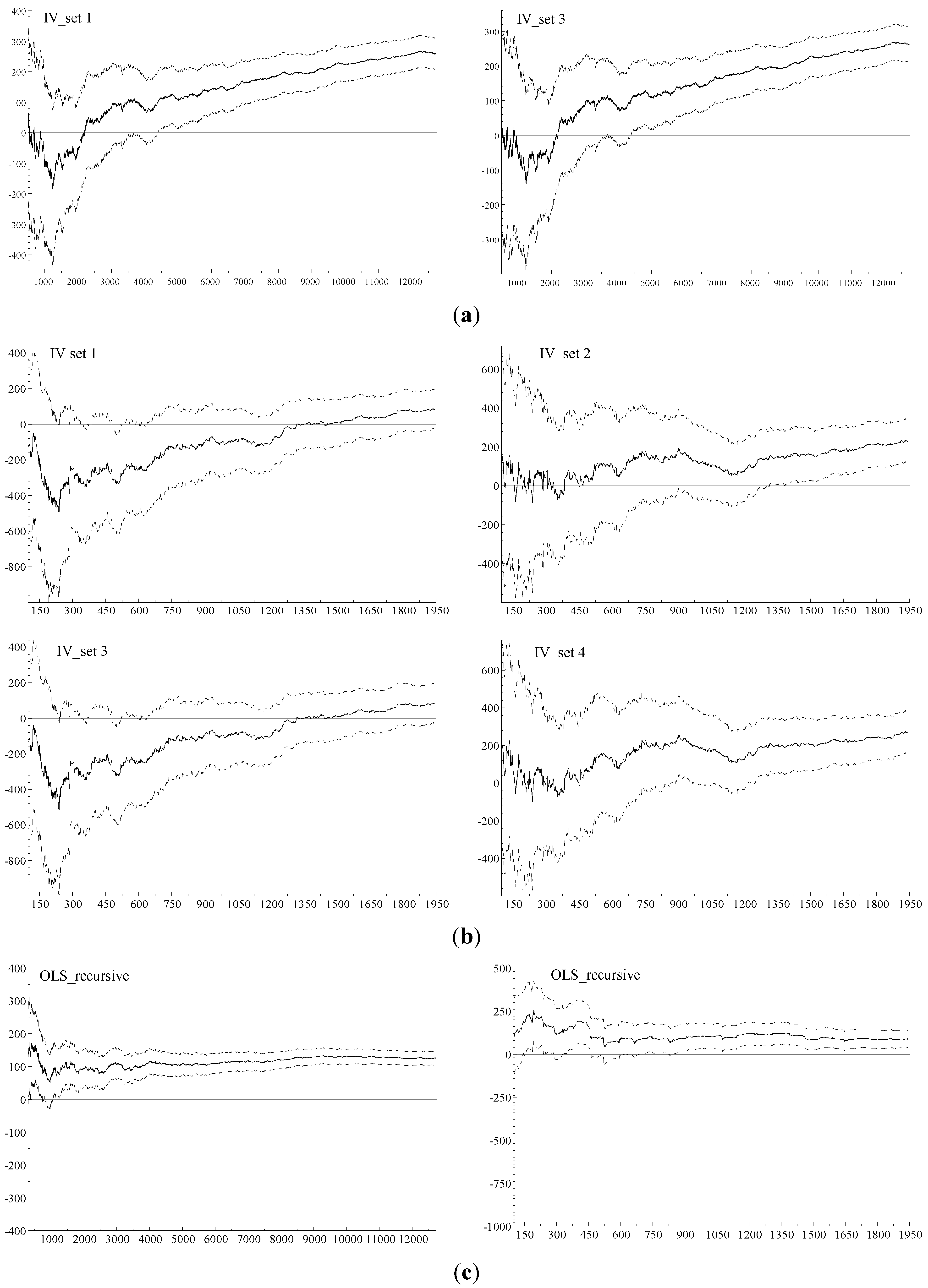
Figure 1 the recursive estimation of
with its 95% confidence interval of the 1999 IV sets reported in
Table 1, together with their counterparts of the OLS estimates (the bottom two graphs). The varied and inaccurate as well as prolific properties of the IV estimates are strikingly obvious, especially in comparison to the OLS plots.
Table 5.
Parameter Stability tests: (i) the first stage regression to generate
; (ii)
of model (2) using the same IV sets as in
Table 1; (iii)
of model (1), full working wife samples.
Table 5.
Parameter Stability tests: (i) the first stage regression to generate ; (ii) of model (2) using the same IV sets as in Table 1; (iii) of model (1), full working wife samples.
| IVs | CPS | PSID | PSID | CPS | PSID | PSID | CPS | PSID |
|---|
| Set 1 | Set 2 | Set 3 | Set 4 | OLS |
|---|
| 1980 | Hansen | 7.714 ** | 0.897 | 1.277 | 11.86 ** | 1.187 | 1.384 | N/A |
| M-fluct. (p-value) | 2.288 ** (0.0000) | 1.236 (0.094) | 0.714 (0.6875) | 2.394 ** (0.0000) | 1.245 (0.0899) | 0.868 (0.4389) | 1.263 (0.0822) | 0.700 (0.7108) |
| 1990 | Hansen | 11.50 ** | 2.760 ** | 3.059 ** | 14.79 ** | 3.713 ** | 3.181 ** | N/A |
| M-fluct. (p-value) | 1.0649 (0.2068) | 1.629 ** (0.0099) | 1.3849 * (0.0432) | 1.0951 (0.1816) | 1.5676* (0.0147) | 1.1185 (0.1637) | 0.9612 (0.3139) | 0.9392 (0.3409) |
| 1999 | Hansen | 10.56 ** | 5.458 ** | 1.8842 | 11.47 ** | 5.974 ** | 1.8770 * | N/A |
| M-fluct. (p-value) | 1.956 ** (0.001) | 1.5463 * (0.0168) | 1.640 ** (0.0092) | 1.966 ** (0.0009) | 1.554 * (0.016) | 1.5426 * (0.0171) | 0.6965 (0.7171) | 0.755 (0.6188) |
| 2003 | Hansen | 8.507 ** | 3.591 ** | 1.9347 * | 9.438 ** | 3.915 ** | 1.8215 * | N/A |
| M-fluct. (p-value) | 2.183 ** (0.0001) | 0.7086 (0.6969) | 0.9672 (0.3069) | 2.180 ** (0.0001) | 0.7596 (0.611) | 0.9239 (0.3606) | 1.638 ** (0.0093) | 1.43 * (0.0334) |
| 2007 | Hansen | 6.293 ** | 2.614 ** | 3.321 ** | 6.903 ** | 3.293 ** | 3.280 ** | N/A |
| M-fluct. (p-value) | 1.2126 (0.1056) | 0.9086 (0.381) | 0.668 (0.7637) | 1.2081 (0.108) | 0.89 (0.4066) | 0.7072 (0.6991) | 1.770 ** (0.0038) | 0.4358 (0.9913) |
| 2011 | Hansen | 7.339 ** | 4.836 ** | 2.0595 * | 7.950 ** | 4.887 ** | 1.8507 * | N/A |
| M-fluct. (p-value) | 1.3061 (0.066) | 0.5972 (0.8679) | 0.6583 (0.779) | 1.3134 (0.0635) | 0.5838 (0.885) | 0.6501 (0.7919) | 1.1847 (0.1208) | 1.6098 * (0.0112) |
Figure 1.
(a) IV Estimation using Current Population Survey (CPS) Data; (b) IV Estimation using Panel Study of Income Dynamics (PSID) Data; (c) OLS Estimation (Left: CPS Data, Right: PSID Data).
Figure 1.
(a) IV Estimation using Current Population Survey (CPS) Data; (b) IV Estimation using Panel Study of Income Dynamics (PSID) Data; (c) OLS Estimation (Left: CPS Data, Right: PSID Data).
The above investigation provides us with abundant evidence to refute
being consistent and refute
being a valid conditional variable instead of
.
9 In other words, we have failed to find adequate and convincing evidence to support the superiority of models (2) and (4) over (1). As a result, the existent IV-based evidence of shrinking elasticities has little credibility.
3. How Can We Find Credible Elasticities?
The above findings are apparently devastating, as they throw us back to the “first generation studies” of labour supply over four decades ago, as described in [
20] (Chapter 11), and pose serious doubts about the micro-econometrics textbook approach. Methodological issues aside, how should we proceed based on the above results?
The preceding within sample parameter stability experiment indicates a possible way forward—sample data ordering. Considering that our focus on
is driven by the need of finding the best possible estimates for the own wage elasticity:
the closest measurement to (5) should be based on the data ordering scheme by
. In other words,
, defined as the percentage change in
in response to a one percent change in
is best reflected when data is order by
so that the incremental change of
is revealed. This ordering scheme clearly satisfies condition (b) stated in the previous section. Condition (a) requires
not to be simultaneously determined by
. Data evidence has failed to show any systematic simultaneity so far (
cf.
Table 4).
With respect to Equation (5), it is obviously better to work with the following log-linear model instead of (1):
The use of semi-log specification in (1) is mainly due to the truncated data feature of
. But since we know that the truncation effect can be reasonably well approximated by scaling the OLS estimates, as shown from
Table 3, we should be able to leave aside the truncation issue for the time being and focus our experiment on data ordering using the working wife sample only.
10Two versions of (1’) are estimated with different specifications of
. For one specification the husband’s wage rate and for the other the family income net of the wife’s earning is used. This is because
is usually the most susceptible to the collinear effect by
among all the explanatory variables in (1’).
11 The resulting
and their related statistics are reported in
Table 6 and
Table 7. It is clear from
Table 6 that different choice of
do not significantly affect
. We thus keep the following modelling experiments on using the family income as
.
The probably most noticeable changes in
Table 7 are the Hansen parameter stability test statistics under different data ordering schemes. The data ordering scheme by
has surely ruined the relative within sample stability of
when data are ordered by wife’s age. It should be noted that although full-sample parameter estimates are invariant to different data ordering schemes, their within-sample recursive processes are not unless there is no hidden dependence between randomly collected cross-section sample observations (see [
43]).
Table 6.
OLS estimates of in model (1’), working wife samples ordered by .
Table 6.
OLS estimates of in model (1’), working wife samples ordered by .
| | | Using Husband Wage Rate | Using Non-wife Family Income |
|---|
| PSID | CPS | PSID | CPS |
|---|
| 1980 | | 0.1054 | 0.0643 ** | 0.0915 | 0.0604 ** |
| 95% C.I.^ | (−0.0315, 0.2423) | (0.0105, 0.1182) | (−0.0439, 0.2268) | (0.0070, 0.1139) |
| AR 1-2 | 23.360 [0.0000] ** | 804.89 [0.0000] ** | 105.97 [0.0000] ** | 795.77 [0.0000] ** |
| Normal. | 1823.1 [0.0000] ** | 21,396 [0.0000] ** | 1810.0 [0.0000] ** | 21,253 [0.0000] ** |
| RESET | 8.8543 [0.0001] ** | 16.824 [0.0000] ** | 6.3416 [0.0018] ** | 25.769 [0.0000] ** |
| 1990 | | 0.1615 ** | 0.2235 ** | 0.1458 ** | 0.2218 ** |
| 95% C.I.^ | (0.0989, 0.2240) | (0.1843, 0.2627) | (0.0846, 0.2071) | (0.1825, 0.2610) |
| AR 1-2 | 43.640 [0.0000] ** | 678.45 [0.0000] ** | 43.999 [0.0000] ** | 676.23 [0.0000] ** |
| Normal. | 3174.6 [0.0000] ** | 27,681 [0.0000] ** | 3155.4 [0.0000] ** | 27,353 [0.0000] ** |
| RESET | 9.5577 [0.0001] ** | 146.46 [0.0000] ** | 10.635 [0.0000] ** | 114.92 [0.0000] ** |
| 1999 | | 0.1305 ** | 0.0947 ** | 0.1219 ** | 0.0926 ** |
| 95% C.I.^ | (0.0546, 0.2064) | (0.0589, 0.1304) | (0.0459, 0.1978) | (0.0571, 0.1280) |
| AR 1-2 | 7.2759 [0.0007] ** | 439.84 [0.0000] ** | 7.5549 [0.0005] ** | 441.26 [0.0000] ** |
| Normal. | 2872.1 [0.0000] ** | 29,232 [0.0000] ** | 2796.9 [0.0000] ** | 29,061 [0.0000] ** |
| RESET | 12.484 [0.0000] ** | 58.163 [0.0000] ** | 10.310 [0.0000] ** | 38.031 [0.0000] ** |
| 2003 | | −0.0193 | 0.0652 ** | −0.0233 | 0.0635 ** |
| 95% C.I.^ | (−0.0992, 0.0606) | (0.0383, 0.0921) | (−0.1015, 0.0549) | (0.0366, 0.0904) |
| AR 1-2 | 26.462 [0.0000] ** | 958.81 [0.0000] ** | 27.154 [0.0000] ** | 952.95 [0.0000] ** |
| Normal. | 3806.7 [0.0000] ** | 51,467 [0.0000] ** | 3771.7 [0.0000] ** | 51,051 [0.0000] ** |
| RESET | 4.7041 [0.0092] ** | 102.35 [0.0000] ** | 2.0922 [0.1237] | 52.963 [0.0000] ** |
| 2007 | | 0.0811 * | 0.0832 ** | 0.0722 * | 0.0773 ** |
| 95% C.I.^ | (0.0135, 0.1487) | (0.0566, 0.1097) | (0.0066, 0.1378) | (0.0512, 0.1035) |
| AR 1-2 | 39.750 [0.0000] ** | 773.51 [0.0000] ** | 41.538 [0.0000] ** | 780.35 [0.0000] ** |
| Normal. | 4043.5 [0.0000] ** | 48,555 [0.0000] ** | 4000.9 [0.0000] ** | 48,375 [0.0000] ** |
| RESET | 10.934 [0.0000] ** | 132.26 [0.0000] ** | 7.4330 [0.0006] ** | 74.285 [0.0000] ** |
| 2011 | | 0.1440 ** | 0.0786 ** | 0.1460 ** | 0.0775 ** |
| 95% C.I.^ | (0.0657, 0.2222) | (0.0501, 0.1071) | (0.0658, 0.2262) | (0.0493, 0.1056) |
| AR 1-2 | 11.143 [0.0000] ** | 882.49 [0.0000] ** | 11.196 [0.0000] ** | 874.96 [0.0000] ** |
| Normal. | 4465.0 [0.0000] ** | 44,067 [0.0000] ** | 4348.3 [0.0000] ** | 43,288 [0.0000] ** |
| RESET | 20.646 [0.0000] ** | 56.446 [0.0000] ** | 18.563 [0.0000] ** | 59.066 [0.0000] ** |
Such hidden dependence can be revealed by appropriate data ordering choice, as shown by Qin and Liu [
36]. Their choice is based on the observation that many economic variables are scale related and that it is frequently too simple to assume a linear/static model between such scale-dependent variables. This linearity assumption amounts to assuming local interdependence or no hidden dependence between observations from the viewpoint of joint probability distribution. Ordering data by the conditional scale-dependent variable of concern serves as an easy way to test this assumption. When the assumption is rejected, the revealed nonlinear effect can be captured by augmenting a static model into a difference-equation model, which captures the gradient of the nonlinear effect much more effectively than the use of conditional scale-dependent variables in a quadratic or cubic form. In the present case, the ordering scheme by wife’s age or by family income largely conceals the hidden nonlinear scale effect by wage rates. This type of ordering schemes is described to as “regime mixing” by Zeileis and Hornik [
34].
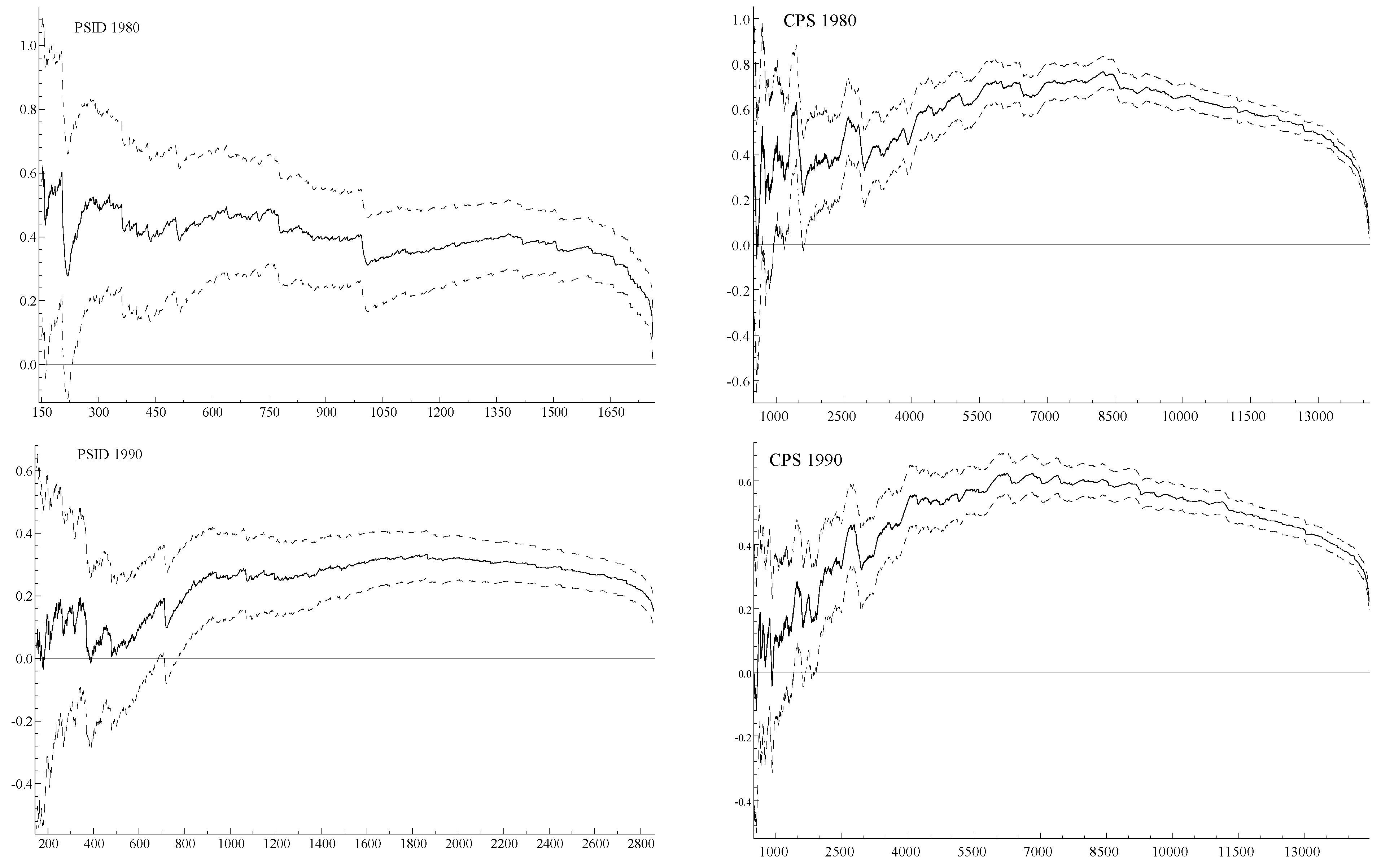
The data ordering effect is best illustrated by comparison of the 1999 OLS recursive estimates, under the ordering scheme by women’s age, presented in
Figure 1 with those of the same wave under the ordering scheme of women’s wage presented in
Figure 2.
Table 7.
Hansen parameter instability test statistics under different data ordering schemes for
in the right two columns of
Table 6.
Table 7.
Hansen parameter instability test statistics under different data ordering schemes for in the right two columns of Table 6.
| Data Source | Ordered by | 1980 | 1990 | 1999 | 2003 | 2007 | 2011 |
|---|
| CPS | Age | 1.4209 ** | 2.0299 ** | 1.5980 ** | 2.0369 ** | 1.8514 ** | 1.7945 ** |
| Income | 0.35413 | 1.5616 ** | 1.0103 ** | 1.7882** | 1.1242 ** | 2.1583 ** |
| Wage | 14.442 ** | 11.990 ** | 10.172 ** | 13.754 ** | 10.596 ** | 10.872 ** |
| PSID | Age | 0.051762 | 0.089821 | 0.093238 | 0.15852 | 0.16041 | 0.46426 |
| Income | 0.22696 | 0.4553 | 0.26751 | 0.17328 | 0.35785 | 0.39903 |
| Wage | 1.0210 ** | 1.5180 ** | 1.1481 ** | 1.4238 ** | 2.1837 ** | 1.8662 ** |
Figure 2.
OLS recursive estimation of in Model (1’) when data are ordered by wage.
Figure 2.
OLS recursive estimation of in Model (1’) when data are ordered by wage.
A striking pattern emerges when we examine and compare the OLS recursive processes of different waves under the ordering scheme by
in
Figure 2. The recursive elasticity estimates follow a somewhat smooth convex curve. Considering the recursive nature of increasing sample sizes, the curves tell us that elasticity of low wage rate earners differs significantly from that of high wage rate earners. This leads us to partition the sample into two parts. The partition wage values are chosen by two considerations. Statistically, they adequately represent the turning points of the convex curves;
12 economically, they are comparable when converted into real-value terms by the US inflation rates. The key results of the partitioned regressions are reported in
Table 8.
Table 8.
OLS estimates of in model (1’) and related statistics, working wife samples partitioned into two, data ordered by .
Table 8.
OLS estimates of in model (1’) and related statistics, working wife samples partitioned into two, data ordered by .
| Data Source | PSID | CPS | PSID | CPS |
|---|
| 1980 | <$5 | >$5 |
| 0.4008 ** | 0.7523 ** | −0.7344 ** | −0.8744 ** |
| 95% C.I.^ | (0.2354, 0.5662) | (0.6793, 0.8254) | (−1.1540, −0.3148) | (−0.9706, −0.7784) |
| Hansen | 0.097470 | 1.2795 ** | 0.79390 ** | 5.4997 ** |
| AR 1-2 | 44.488 [0.0000] ** | 259.18 [0.0000] ** | 42.455 [0.0000] ** | 232.38 [0.0000] ** |
| Normal. | 598.05 [0.0000] ** | 9105.4 [0.0000] ** | 1260.2 [0.0000] ** | 7108.9 [0.0000] ** |
| RESET | 4.0836 [0.0171] * | 18.388 [0.0000] ** | 22.236 [0.0000] ** | 112.47 [0.0000] ** |
| 1990 | <$8 | >$8 |
| 0.2780 ** | 0.6017 ** | −0.3489 ** | −0.4034 ** |
| 95% C.I.^ | (0.0912, 0.2005) | (0.5341, 0.6693) | (−0.4933, −0.2044) | (−0.4818, −0.3251) |
| Hansen | 0.24888 | 1.1302 ** | 0.43981 | 3.6915 ** |
| AR 1-2 | 28.174 [0.0000] ** | 203.75 [0.0000] ** | 4.0878 [0.0170]* | 304.19 [0.0000] ** |
| Normal. | 1160.6 [0.0000] ** | 8186.1 [0.0000] ** | 1908.7 [0.0000] ** | 16,933 [0.0000] ** |
| RESET | 4.6074 [0.0101] * | 24.824 [0.0000] ** | 25.942 [0.0000] ** | 92.994 [0.0000] ** |
| 1999 | <$10 | >$10 |
| 0.3601 ** | 0.3489 ** | −0.1304* | −0.3361 ** |
| 95% C.I.^ | (0.1836, 0.5366) | (0.2824, 0.4153) | (−0.2557, −0.0050) | (−0.4020, −0.2702) |
| Hansen | 0.083408 | 0.39901 | 0.25306 | 2.1439 ** |
| AR 1-2 | 3.2069 [0.0410] * | 114.53 [0.0000] ** | 1.6441 [0.1936] | 214.87 [0.0000] ** |
| Normal. | 581.82 [0.0000] ** | 7568.7 [0.0000] ** | 2086.3 [0.0000] ** | 15,967 [0.0000] ** |
| RESET | 1.0228 [0.3601] | 21.939 [0.0000] ** | 5.4624 [0.0044] ** | 89.717 [0.0000] ** |
| 2003 | <$11 | >$11 |
| 0.1976 ** | 0.3225 ** | −0.4171 ** | −0.2890 ** |
| 95% C.I.^ | (0.0544, 0.3408) | (0.2687, 0.3762) | (−0.5696, −0.2646) | (−0.3360, −0.2420) |
| Hansen | 0.066383 | 1.1583 ** | 0.45268 | 3.4500 ** |
| AR 1-2 | 4.2232 [0.0150] * | 257.47 [0.0000] ** | 12.054 [0.0000] ** | 492.32 [0.0000] ** |
| Normal. | 409.73 [0.0000] ** | 9296.9 [0.0000] ** | 3580.2 [0.0000] ** | 36,000 [0.0000] ** |
| RESET | 0.6505 [0.5221] | 20.417 [0.0000] ** | 28.754 [0.0000] ** | 160.74 [0.0000] ** |
| 2007 | <$13 | >$13 |
| 0.3395 ** | 0.3299 ** | −0.2396 ** | −0.2367 ** |
| 95% C.I.^ | (0.1855, 0.4934) | (0.2783, 0.3814) | (−0.3424, −0.1368) | (−0.2841, −0.1894) |
| Hansen | 0.45521 | 0.47376 * | 0.093207 | 1.2606 ** |
| AR 1-2 | 15.908 [0.0000] ** | 238.84 [0.0000] ** | 9.4808 [0.0001] ** | 372.39 [0.0000] ** |
| Normal. | 891.89 [0.0000] ** | 9769.9 [0.0000] ** | 2507.1 [0.0000] ** | 34,758 [0.0000] ** |
| RESET | 2.1334 [0.1191] | 22.140 [0.0000] ** | 7.1945 [0.0008] ** | 77.495 [0.0000] ** |
| 2011 | <$13.50 | >$13.50 |
| 0.3278 ** | 0.3330 ** | −0.2057 ** | −0.2517 ** |
| 95% C.I.^ | (0.1452, 0.5105) | (0.2756, 0.3904) | (−0.3452, −0.0663) | (−0.3015, −0.2019) |
| Hansen | 0.16577 | 1.1026 ** | 0.35168 | −10.1 ** |
| AR 1-2 | 6.4511 [0.0017] ** | 241.38 [0.0000] ** | 0.2538 [0.7759] | 445.02 [0.0000] ** |
| Normal. | 803.83 [0.0000] ** | 7703.4 [0.0000] ** | 3244.4 [0.0000] ** | 31,573 [0.0000] ** |
| RESET | 0.6919 [0.5009] | 22.142 [0.0000] ** | 32.758 [0.0000] ** | 120.92 [0.0000] ** |
Four features are immediately noticeable from this table as compared to the previous estimation results summarised in
Table 6 and
Table 7. First, there is little statistical difference between the elasticity estimates of the two data sources for most of the waves. Secondly, the elasticity estimates of the lower part are significantly positive whereas those of the upper part are significantly negative. Thirdly, there are signs of reducing severity of the diagnostic test rejections, mainly from the PSID source. Fourthly, parameter instability is still largely present, especially for estimates using the CPS source, as shown by the Hansen test statistics. Inspection of recursive estimation results tells us that the instability mostly occurs at the tail ends of the wage distribution. Therefore, we further partition the two subsamples to cut out the tail ends, aiming to search for the comparable wage rate ranges within which the elasticity estimates remain statistically constant. The search yields a comparable wage range of $4–$10 from the lower end and $10–$22 from the upper end at the 1999 price level. We refer to these two partition ranges as the lower mid group and the upper mid group in
Table 9, where the main results of this search are summarised.
Two key changes are discernible from
Table 8 to
Table 9. The elasticity estimates of the upper mid group are statistically insignificant from zero, and all the estimates in the lower mid group have passed the Hansen stability test whereas only two have failed the test in the upper mid group.
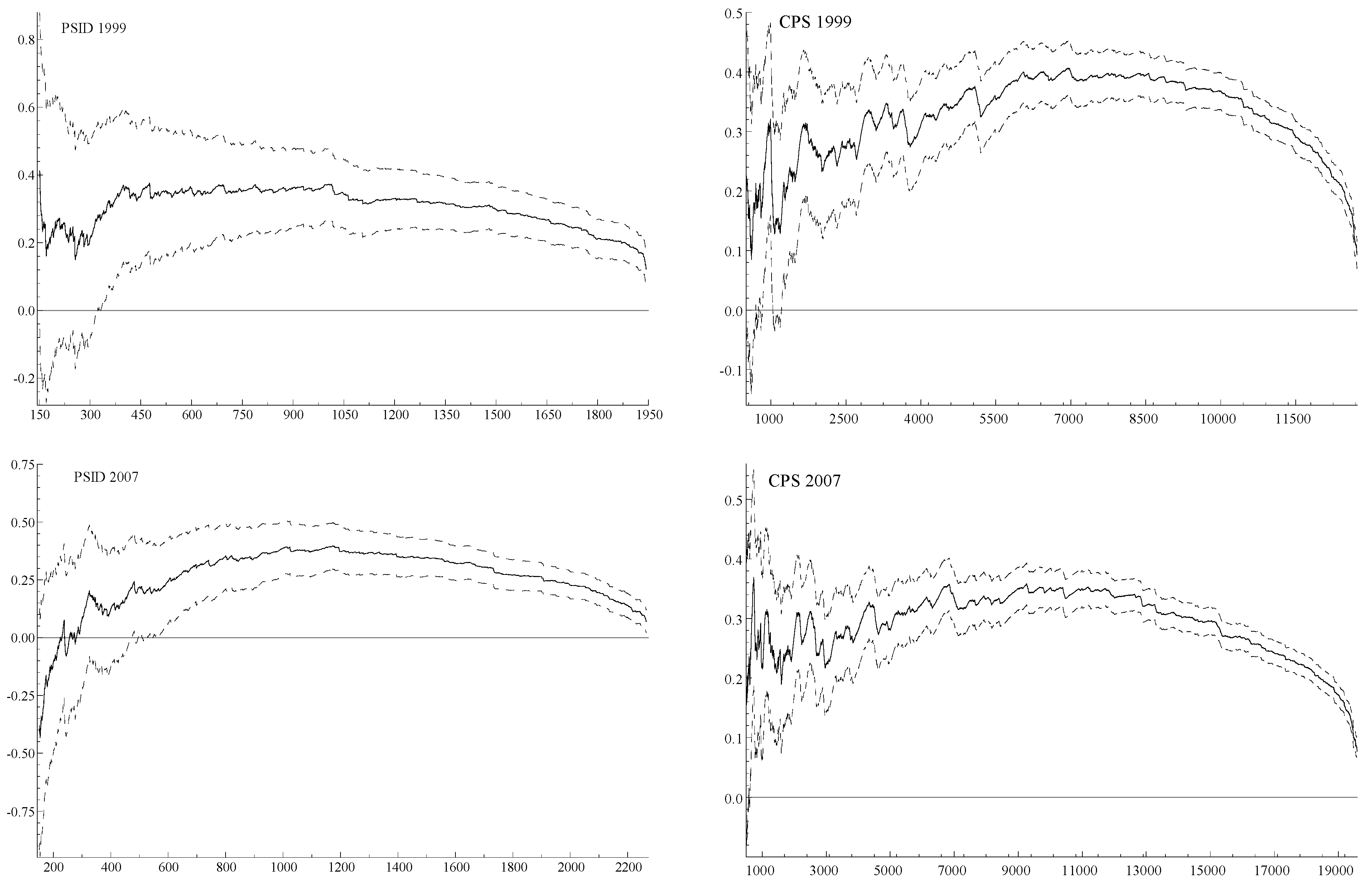
Figure 3 plots all the OLS recursive graphs of the lower mid group. The degree of parameter stability is quite impressive, especially considering the large sample sizes of the CPS source. However, what is even more impressive is the closeness of these elasticity estimates—roughly around 0.4—not only between the two data sources of the same wave but also across different waves, especially the last four waves.
Table 9.
OLS estimates of in model (1’) and related statistics, working wife samples partitioned into lower mid and upper mid groups, plus RAL estimates for autocorrelated residual correction of the lower mid group, data ordered by .
Table 9.
OLS estimates of in model (1’) and related statistics, working wife samples partitioned into lower mid and upper mid groups, plus RAL estimates for autocorrelated residual correction of the lower mid group, data ordered by .
| | Lower Mid Group | Upper Mid Group |
|---|
| PSID | CPS | PSID | CPS |
|---|
| OLS | RAL | OLS | RAL | OLS | OLS |
|---|
| 1980 | $2.00–$5.00 | $5.00–$10.50 |
| 0.3297 * | 0.2924 | 0.9236 ** | 0.9312 ** | 0.2681 | −0.1175 |
| 95% C.I.^ | (0.03, 0.63) | (−0.07, 0.65) | (0.83, 1.02) | (0.82, 1.05) | (−0.09, 0.63) | (−0.26, 0.03) |
| Hansen | 0.066046 | | 0.25999 | | 0.38964 | 1.1773 ** |
| AR 1-2 | 35.5 [0.00] | 749 [0.00] | 237.8 [0.00] | 8366 [0.00] | 44.64 [0.00] | 200.80 [0.00] |
| Normal. | 661 [0.00] | 9667 [0.00] | 1074 [0.00] | 10,157 [0.00] |
| RESET | 3.73 [0.02] | 10.59 [0.00] | 3.848 [0.02] | 7.1779 [0.00] |
| 1990 | $3.00–$8.00 | $8.00–$17.00 |
| 0.4124 ** | 0.4075 ** | 0.7719 ** | 0.7718 ** | −0.0755 | 0.0375 |
| 95% C.I.^ | (0.25, 0.58) | (0.21, 0.61) | (0.69, 0.86) | (0.67, 0.88) | (−0.25, 0.10) | (−0.06, 0.13) |
| Hansen | 0.063294 | | 0.36629 | | 0.024241 | 0.15996 |
| AR 1-2 | 37.54 [0.00] | 1292 [0.00] | 170.1 [0.00] | 7629 [0.00] | 9.350 [0.00] | 224.4 [0.00] |
| Normal. | 1207 [0.00] | 8698 [0.00] | 1675 [0.00] | 17,938 [0.00] |
| RESET | 5.577 [0.00] | 17.76 [0.00] | 5.657 [0.00] | 15.07 [0.00] |
| 1999 | $4.00–$10.00 | $10.00–$22.00 |
| 0.5095 ** | 0.5098 ** | 0.3916 ** | 0.3936 ** | 0.1129 | 0.0668 |
| 95% C.I.^ | (0.26, 0.76) | (0.25, 0.77) | (0.29, 0.49) | (0.28, 0.51) | (−0.05, 0.28) | (−0.02, 0.15) |
| Hansen | 0.069269 | | 0.30388 | | 0.067335 | 0.66744 * |
| AR 1-2 | 3.15 [0.04] | 674.6 [0.00] | 95.10 [0.00] | 7523 [0.00] | 1.119 [0.33] | 174.3 [0.00] |
| Normal. | 692.8 [0.00] | 8097 [0.00] | 1769.5 [0.00] | 16,403 [0.00] |
| RESET | 2.363 [0.10] | 20.59 [0.00] | 12.55 [0.00] | 13.450 [0.00] |
| 2003 | $4.50–$11.00 | $11.00–$24.00 |
| 0.2071 | | 0.4530 ** | 0.4542 ** | −0.0142 | 0.0248 |
| 95% C.I.^ | (−0.02, 0.44) | | (0.37, 0.54) | (0.35, 0.56) | (−0.17, 0.14) | (−0.04, 0.09) |
| Hansen | 0.051773 | | 0.29838 | | 0.095798 | 0.33216 |
| AR 1-2 | 2.787 [0.06] | | 255.3 [0.00] | 8559 [0.00] | 6.5423 [0.00] | 297.37 [0.00] |
| Normal. | 328.0 [0.00] | 10,014 [0.00] | 2418.1 [0.00] | 31,624 [0.00] |
| RESET | 2.079 [0.13] | 22.15 [0.00] | 1.3935 [0.25] | 32.201 [0.00] |
| 2007 | $5.00–$13.00 | $13.00–$27.00 |
| 0.6299 ** | 0.6347 ** | 0.4295 ** | 0.424609 ** | −0.1118 | −0.0239 |
| 95% C.I.^ | (0.36, 0.90) | (0.31, 0.96) | (0.36, 0.50) | (0.34, 0.51) | (−0.28, 0.05) | (−0.09, 0.04) |
| Hansen | 0.046116 | | 0.26206 | | 0.063481 | 0.28024 |
| AR 1-2 | 18.53 [0.00] | 899.7 [0.00] | 229.09 [0.00] | 9526 [0.00] | 19.088 [0.00] | 311.17 [0.00] |
| Normal. | 889.4 [0.00] | 10,816 [0.00] | 2012.6 [0.00] | 28,177 [0.00] |
| RESET | 1.597 [0.20] | 34.515 [0.00] | 10.836 [0.00] | 7.1955 [0.00] |
| 2011 | $5.50–$13.50 | $13.50–$29.50 |
| 0.4793 ** | 0.4859 ** | 0.4349 ** | 0.4323 ** | 0.0901398 | 0.0053 |
| 95% C.I.^ | (0.18, 0.78) | (0.18, 0.80) | (0.35, 0.53) | (0.32, 0.55) | (−0.07, 0.25) | (−0.06, 0.07) |
| Hansen | 0.13927 | | 0.30747 | | 0.020069 | 0.36278 |
| AR 1-2 | 6.497 [0.00] | 806.7 [0.00] | 224.95 [0.00] | 7364 [0.00] | 0.9746 [0.38] | 234.79 [0.00] |
| Normal. | 920.9 [0.00] | 8782.1 [0.00] | 2407.3 [0.00] | 22,546 [0.00] |
| RESET | 1.180 [0.31] | 18.097 [0.00] | 1.5094 [0.22] | 24.795 [0.00] |
Since the lower mid group stands out as having the most stable and significantly positive wage elasticity estimates, we try to further investigate the robustness of this finding from two aspects. First, we run the reverse regression model, namely the upper equation in (4) with data ordered by
and try the same sample partition search to see if it is possible to find ranges of work hours in which relatively invariant parameter estimates of
exist. This experiment can be seen as a crosscheck of whether
satisfies data ordering condition (a). The search yields no positive results, as shown in
Table 10. The universal lack of parameter stability and the statistical similarity between the two data sources across different waves serve as strong evidence against postulating
as a conditional variable for
.
Figure 3.
Recursive estimation of for the lower mid group, data ordered by wage.
Figure 3.
Recursive estimation of for the lower mid group, data ordered by wage.
Table 10.
OLS estimates of in the lower equation of (4) and related statistics, full working wife samples and subsamples in various partitions, data ordered by .
Table 10.
OLS estimates of in the lower equation of (4) and related statistics, full working wife samples and subsamples in various partitions, data ordered by .
| | | 1980 | 1990 | 1999 | 2003 | 2007 | 2011 |
|---|
| Full sample |
| PSID | | 0.00008 ** | 0.00008 ** | 0.000064 * | −0.000008 | 0.000035 | 0.00007 ** |
| p-value of t-test^ | 0.0003 | 0.0000 | 0.0122 | 0.6356 | 0.1174 | 0.0054 |
| Hansen test | 0.5524 * | 1.5082 ** | 1.1711 ** | 0.5951 * | 0.5064 * | 1.6662 ** |
| CPS | | 0.00006 ** | 0.00012 ** | 0.00008 ** | 0.00006 ** | 0.00007 ** | 0.00008 ** |
| p-value of t-test^ | 0.0000 | 0.0000 | 0.0000 | 0.0000 | 0.0000 | 0.0000 |
| Hansen test | 59.27 ** | 55.4 ** | 61.4 ** | 98.3 ** | 103.1 ** | 94.53 ** |
| Part-timers |
| 1–1680 h per year |
| PSID | | 0.000095 * | 0.00011 ** | 0.00016 ** | 0.000001 | 0.000098 | 0.00019 ** |
| p-value of t-test^ | 0.0284 | 0.0029 | 0.0077 | 0.9788 | 0.0617 | 0.0005 |
| Hansen test | 0.0947 | 0.2481 | 0.0262 | 0.9170 * | 0.1231 | 0.0837 |
| CPS | | −0.0001 ** | 0.00008 ** | −0.000032 | −0.000006 | 0.000018 | −0.000004 |
| p-value of t-test^ | 0.0020 | 0.0000 | 0.1704 | 0.7252 | 0.3949 | 0.8688 |
| Hansen test | 2.36 ** | 1.01 ** | 1.82 ** | 4.33 ** | 4.23 ** | 3.29 ** |
| 1–1000 h per year |
| PSID | | 0.000006 | −0.000016 | 0.00027 | −0.0005 ** | 0.000097 | 0.00015 |
| p-value of t-test^ | 0.9573 | 0.8694 | 0.1122 | 0.0018 | 0.4870 | 0.3376 |
| Hansen test | 0.3851 | 0.1088 | 0.0807 | 0.1591 | 0.0893 | 0.1349 |
| CPS | | −0.0002 ** | 0.000021 | −0.0002 ** | −0.0002 ** | −0.0002 ** | −0.000266 |
| p-value of t-test^ | 0.0000 | 0.6316 | 0.0028 | 0.0000 | 0.0007 | 0.0000 |
| Hansen test | 0.91 ** | 0.27 | 0.62 * | 2.28 ** | 1.19 ** | 1.58 ** |
| 1000–1680 h per year |
| PSID | | −0.00007 | 0.00028 * | 0.000126 | 0.00046 ** | 0.00037 ** | 0.00024 |
| p-value of t-test^ | 0.5874 | 0.0178 | 0.3496 | 0.0039 | 0.0081 | 0.0699 |
| Hansen test | 0.0319 | 0.0931 | 0.0263 | 0.0824 | 0.1016 | 0.0721 |
| CPS | | 0.000052 | 0.000038 | 0.00021 ** | −0.000004 | 0.000088 | −0.000025 |
| p-value of t-test^ | 0.1747 | 0.4114 | 0.0001 | 0.9199 | 0.0575 | 0.5846 |
| Hansen test | 1.80 ** | 2.26 ** | 2.03 ** | 4.80 ** | 3.76 ** | 3.16 ** |
| Full-timers |
| >1680 h per year (35 h per week) |
| PSID | | −0.0002 ** | −0.0002 ** | −0.0001 ** | −0.0002 ** | −0.00007 | −0.0002 ** |
| p-value of t-test^ | 0.0045 | 0.0000 | 0.0070 | 0.0000 | 0.1505 | 0.0000 |
| Hansen test | 0.1520 | 0.2044 | 0.1392 | 0.3486 | 0.0923 | 0.2045 |
| CPS | | −0.000041 | −0.000032 | −0.000020 | −0.0001 ** | −0.0001 ** | −0.0001 ** |
| p-value of t-test^ | 0.1400 | 0.2088 | 0.4203 | 0.0004 | 0.0076 | 0.0041 |
| Hansen test | 124.1 ** | 132.2 ** | 107.0 ** | 185.5 ** | 190.0 ** | 174.4 ** |
| 1680–2400 h per year (35–50 h per week) |
| PSID | | −0.00006 | −0.0001 | −0.0003 ** | −0.00032 | −0.000054 | −0.00021 |
| p-value of t-test^ | 0.5663 | 0.2303 | 0.0016 | 0.7047 | 0.5250 | 0.0512 |
| Hansen test | 0.2151 | 0.2549 | 0.1329 | 0.2457 | 0.1830 | 0.2289 |
| CPS | | 0.00026 ** | 0.00031 ** | 0.00035 ** | 0.00021 ** | 0.00035 ** | 0.00028 ** |
| p-value of t-test^ | 0.0000 | 0.0000 | 0.0000 | 0.0000 | 0.0000 | 0.0000 |
| Hansen test | 132.1 ** | 151.7 ** | 144.4 ** | 261.1 ** | 264.0 ** | 248.5 ** |
The second aspect is to tackle the residual autocorrelation problem, which is widely observed from the diagnostic tests shown in
Table 9. The autocorrelation actually indicates the presence of hidden dependence or nonlinear scale effect, as discussed above. Here, we re-estimate the model using the Cochrane-Orcutt autoregressive least-squares method for those instances where the OLS regression fails the residual AR test. Interestingly, the resulting elasticity estimates do not differ statistically from the OLS estimates, as shown in
Table 9. This finding indicates that the nonlinear effect by data ordering satisfies the common factor restriction, e.g., see [
44] (Chapter 7). In other words, the “short-run” wage effect is identical to the “long-run” wage effect. This is not very surprising considering that the “short-run” of the present case is the wage rate incremental (see [
36] for more discussion on this point).
The discovery of constant elasticity estimates in two sub-groups of working wives leads us to another experiment of the IV route to see how invariant the two sub-group IV estimates are, using un-ordered subsample data.
13 Table 11 summarises the results.
Table 11.
IV estimates of in model (2) and related statistics, for two wage rate sub-samples.
Table 11.
IV estimates of in model (2) and related statistics, for two wage rate sub-samples.
| IVs | Set 1 | Set 3 |
|---|
| CPS | PSID | CPS | PSID | CPS | PSID | CPS | PSID |
|---|
| Wage Group | Lower Mid | Upper Mid | Lower Mid | Upper Mid |
|---|
| 1980 | | −51.826 | −3518.1 | 1411. ** | −49.47 | −135.85 | −3510.9 | 1612 ** | −18.54 |
| R.S.E. | 263.85 | 1897 | 276.376 | 445.18 | 261.266 | 1895.5 | 280.43 | 445.87 |
| Hausman | 9.392 ** | 11.26 ** | 29.63 ** | 0.1549 | 11.95 ** | 11.23 ** | 39.85 ** | 1.0 |
| Over-id. | 71.77 ** | 8.2155 | 48.15 ** | 4.7803 | 75.12 ** | 8.2446 | 67.98 ** | 7.28 |
| 1990 | | −652.9 * | −1568 * | 1137 ** | −44.698 | −513.47 | −1487 * | 1180 ** | −78.07 |
| R.S.E. | 311.703 | 741.98 | 153.698 | 319.83 | 300.071 | 728.6 | 154.725 | 318.1 |
| Hausman | 20.53 ** | 12.35 ** | 57.65 ** | 0.0459 | 16.75 ** | 11.42 ** | 63.33 ** | 0.119 |
| Over-id. | 30.39 ** | 8.145 ** | 25.67 ** | 22.06 ** | 38.72 ** | 10.83 | 34.8 ** | 22.27 ** |
| 1999 | | −2082 ** | 424.863 | 920.9 ** | −547.64 | −1991 ** | 498.2 | 964.2 ** | −444.88 |
| R.S.E. | 496.4 | 526.58 | 148.82 | 510.58 | 477.99 | 520.5 | 151.09 | 496.87 |
| Hausman | 43.62 ** | 0.0001 | 35.03 ** | 2.255 | 41.65 ** | 0.019 | 39.41 ** | 1.686 |
| Over-id. | 14.92 ** | 22.7 ** | 46.44 ** | 14.61 ** | 16.60 ** | 26.85 ** | 54.46 ** | 16.19 ** |
| 2003 | | −1309 ** | −842.97 | 682.3 ** | 848.2 | −1247 ** | −1121.4 | 672. 3 ** | 852.76 |
| R.S.E. | 439.18 | 1511.2 | 122.444 | 443.1 | 433.67 | 1485.6 | 121.76 | 443.5 |
| Hausman | 19.03 ** | 0.69 | 29.88 ** | 4.9396 * | 17.78 ** | 1.171 | 28.97 ** | 4.994 * |
| Over-id. | 55.33 ** | 17.27 ** | 84.51 ** | 5.71 | 59.52 ** | 16.52 ** | 89.27 ** | 6.82 |
| 2007 | | −930 ** | 787.93 | 1122 ** | −418.53 | −814 ** | 828.88 | 1121 ** | −418.12 |
| R.S.E. | 254.88 | 764.98 | 138.28 | 499.7 | 247.91 | 758.93 | 137.83 | 497.5 |
| Hausman | 33.05 ** | 0.10 | 72.52 ** | 0.35 | 28.18 ** | 0.1456 | 72.44 ** | 0.35 |
| Over-id. | 38.37 ** | 8.99 | 65.57 ** | 19.12 ** | 48.75 ** | 9.12 | 65.66 ** | 19.12 ** |
| 2011 | | −918.3 * | 1916.6 * | 1238 ** | 919.28 * | −517.98 | 1910 * | 1226 ** | 932.83 * |
| R.S.E. | 371.07 | 958.3 | 130.33 | 449.2 | 342.82 | 975.17 | 128.88 | 450.38 |
| Hausman | 13.54 ** | 2.42 | 103.9 ** | 4.442 * | 7.22 ** | 2.40 | 102.3 ** | 4.58 * |
| Over-id. | 19.73 ** | 3.29 | 92.39 ** | 11.67 * | 37.53 ** | 3.32 | 94.6 ** | 13.56 * |
It is striking to see from the table that all the CPS data-based IV estimates for the lower mid wage group are now negative whereas the estimates for the upper mid wage group are several times larger than the full-sample estimates as compared to
Table 1. This result is contrary to the expectation that the elasticity of lower wage earners should be positive and larger than that of the higher wage earners. Unsurprisingly, all the IV test results remain unchanged from the full-sample results for the CPS data sets, with the Sargan test rejecting the validity of all the IV sets. The IV test results using the PSID data sets vary somewhat from those reported in
Table 1. Interestingly, some test results alter between wage groups for the same IV sets, e.g., endogeneity is rejected in the upper wage group but not the lower wage group in 1980, and
vice versa in 2003. These cases show us again how unreliable IV-generated wage variables can be when used as conditional variables. The degree of variedness in those sub-group IV estimates using the PSID data sets is not beyond expectation. On the whole, the cross-sample time-invariant feature revealed by the OLS estimates is absent here.
The above findings not only reconfirm our rejection of models (2) and (4), but also carry a great deal of practical significance, at least from the following five aspects.
The first and obvious implication of our findings is that wage elasticity for the working wives is not a single-valued parameter. The evidence from
Table 9 that statistically constant elasticities exist only with respect to certain wage groups undermines the premise of the labour supply wage effect as a single parameter using micro data. Consequently, a theoretical re-orientation is probably needed for those investigations which are aimed at establishing links between macro and micro labour supply elasticities. These findings also support more heterodox theories of labour market segmentation, e.g., [
45,
46], and show potential avenues for future empirical research in this field.
Secondly, there is little evidence of shrinking wage elasticities from 1980 to 2011 as far as those statistically constant elasticities are concerned. On the contrary, these estimates have remained remarkably invariant, as shown in
Table 9. Although some sign of decreasing elasticities is discernible from the CPS-based estimates of the three waves of 1980, 1990 and 1999, the decrease is statistically too weak to support the claim of shrinking elasticities. If we look at the aggregate estimates from
Table 1,
Table 2,
Table 3,
Table 4,
Table 5 and
Table 6, differences in the wage elasticity estimates are somewhat more noticeable from these three waves. In order to find explanations to this phenomenon, we look into the share compositions of working wives by our sample partitions. What we find is a significant decline in the shares of the lower mid group combined with a significant increase in the shares of the upper mid group as well as the upper part from 1980 to 1999, whereas the shares have largely stabilised since 1999, as shown from
Figure 4.
Figure 4.
Lower and Upper Mid Wife Wage Group Share in Total (CPS and PSID, in percentage, 1980–2011).
Figure 4.
Lower and Upper Mid Wife Wage Group Share in Total (CPS and PSID, in percentage, 1980–2011).
Since the lower mid group is the only one where stable and significantly positive elasticities are found to hold whereas the upper part of the sample contributes to negate the presence of a positive elasticity, it is no wonder that a shrinking elasticity phenomenon has been observed from aggregate sample estimations of the 1980–2000 period. This finding tells us that what has changed over time is not wage elasticities with respect to the lower and upper mid groups, but the distribution of working wives in relatively lower paid jobs. This is in line with Juhn and Murphy’s [
8] observation of increasing wage opportunities for women as well as findings by Welch [
47] on a weakening segregation between male and female labour markets by wage rate. This development is further revealed by the shifting distributions of wife’s wage rates from 1980 to 2011 as compared to the distributions of husband’s wage, see
Figure 5. The distributions of wage rates by gender have clearly been converging over the last three decades.
Thirdly, the finding of the two groups within which statistically constant elasticities are present provides us with a new angle to tackle the sample selection bias concern with respect to sample representativeness. Our recursive partition search identifies the tail ends of the female wage rates in the full-working wife samples as being largely at odd with the rest of the sample. From the practical viewpoint of finding sample evidence which would be representative of the population concerned and thus endorses statistical inference, we should partition out the tail end non-representative observations as judged by the a priori conditional theory of interest, so as to tighten the conditional range upon which statistical inferences are made. It should be noted also that this research strategy carries special implication to models using panel data. Since most of panel-data based models assume single valued parameters of interest, it is vital to exclude individual elements in the panel which are far from representative of the population of interest. Failure of such exclusion would result in sample selection bias.
Figure 5.
Distribution of Wife’s and Husbands’ Wage Rate in 1980 and 2011 (hourly wage in log, Left: frequency, Right: normal density).
Figure 5.
Distribution of Wife’s and Husbands’ Wage Rate in 1980 and 2011 (hourly wage in log, Left: frequency, Right: normal density).
Fourthly, the finding that there is no single-valued wage elasticity across the wage earners suggests that it could be over-simplistic to treat the non-working wives as a homogenous group and carry out empirical investigation on aggregate extensive margins by means of binary regression models. From the viewpoint of measuring wage elasticity for labour participation, disaggregate studies may be better off partitioning data by wage rate ranges rather than labour participation types. Since our wage imputation method is based on the idea of counterfactual matching of comparable groups, we can exploit the constant elasticity based sample partitions to examine how the imputed wage rates are distributed. It is seen from
Table 12 that the percentage of imputed wage rates of non-working wives falling into the lower part of the wage partition is generally higher than that of non-working wives falling into the upper part. Clearly, more experiments are needed to evaluate the robustness of those imputed wages.
Table 12.
Wage distribution of the imputed offering wage rates for nonworking women, percentage shares calculated by the partitions given in
Table 8 and
Table 9.
Table 12.
Wage distribution of the imputed offering wage rates for nonworking women, percentage shares calculated by the partitions given in Table 8 and Table 9.
| | PSID | CPS |
|---|
| Lower Part | Upper Part | Lower Mid Group | Upper Mid Group | Lower Part | Upper Part | Lower Mid Group | Upper Mid Group |
|---|
| 1980 | 84.77% | 15.23% | 78.52% | 13.80% | 68.86% | 31.14% | 68.11% | 30.95% |
| 1990 | 89.83% | 10.17% | 70.10% | 8.47% | 76.82% | 23.18% | 74.80% | 22.78% |
| 1999 | 75.71% | 24.29% | 69.37% | 19.26% | 60.93% | 39.07% | 60.69% | 37.37% |
| 2003 | 76.67% | 23.33% | 71.49% | 19.01% | 46.12% | 54.09% | 45.91% | 50.09% |
| 2007 | 76.09% | 23.91% | 71.10% | 17.88% | 53.77% | 46.48% | 53.52% | 41.12% |
| 2011 | 83.60% | 16.40% | 71.08% | 14.46% | 50.61% | 49.99% | 50.01% | 45.94% |
Table 13.
Probit estimates of the wage coefficient in labour force participation regressions.
Table 13.
Probit estimates of the wage coefficient in labour force participation regressions.
| Samples | Full | Lower Mid Wage Group | Upper Quarter of the Lower Mid Group | Upper Mid Wage Group |
|---|
| PSID | CPS | PSID | CPS | CPS | PSID | CPS |
|---|
| 1980 | | 0.486 ** | 0.0738 ** | 1.409 ** | −0.459 ** | 0.821 | 1.514 ** | 1.710 ** |
| 95% C.I.^ | (0.4, 0.6) | (0.03, 0.1) | (1.1, 1.7) | (−0.6, −0.4) | (−0.2, 1.8) | (0.8, 2.2) | (1.5, 1.9) |
| Elasticity | 0.1833 ** | 0.0380 ** | 0.517 ** | −0.211 ** | 0.451 | 0.521 ** | 0.984 ** |
| 95% C.I.^ | (0.14, 0.2) | (0.02, 0.1) | (0.41, 0.6) | (−0.3, −0.2) | (−0.1, 1.0) | (0.3, 0.7) | (0.9, 1.1) |
| 1990 | | 0.6824 ** | 0.382 ** | 1.478 ** | 0.169 ** | 3.763 ** | 1.2456 ** | 0.760 ** |
| 95% C.I.^ | (0.6, 0.8) | (0.3, 0.4) | (1.2, 1.7) | (0.1, 0.3) | (2.7, 4.8) | (0.6, 1.9) | (0.6, 0.9) |
| Elasticity | 0.26 ** | 0.219 ** | 0.652 ** | 0.101 ** | 2.313 ** | 0.2878 ** | 0.408 ** |
| 95% C.I.^ | (0.2, 0.3) | (0.2, 0.24) | (0.55, 0.8) | (0.04, 0.2) | (1.67, 3.0) | (0.14, 0.4) | (0.32, 0.5) |
| 1999 | | 0.658 ** | 0.230 ** | 1.1825 ** | −2.008 ** | 1.145 | 1.076 ** | 1.651 ** |
| 95% C.I.^ | (0.54, 0.8) | (0.18, 0.3) | (0.8, 1.54) | (−2.2, −1.8) | (−0.1, 2.3) | (0.5, 1.7) | (1.5, 1.8) |
| Elasticity | 0.318 ** | 0.153 ** | 0.664 ** | −1.280 ** | 0.922 | 0.3849 ** | 1.030 ** |
| 95% C.I.^ | (0.27, 0.4) | (0.12, 0.2) | (0.5, 0.85) | (−1.4, −1.2) | (−0.03, 2) | (0.18, 0.6) | (0.92, 1.1) |
| 2003 | | 0.8848 ** | 0.191 ** | 1.4856 ** | −3.858 ** | −1.893 ** | 1.477 ** | 1.710 ** |
| 95% C.I.^ | (0.77, 1.0) | (0.16, 0.2) | (1.1, 1.86) | (−4.1, −3.6) | (−2.8, −1) | (0.83, 2.1) | (1.58, 1.8) |
| Elasticity | 0.422 ** | 0.142 ** | 0.9573 ** | −2.247 ** | −1.662 ** | 0.4534 ** | 1.253 ** |
| 95% C.I.^ | (0.37, 0.5) | (0.12, 0.2) | (0.74, 1.2) | (−2.4, −2.1) | (−2.5, −1) | (0.26, 0.7) | (1.16, 1.3) |
| 2007 | | 0.811 ** | 0.195 ** | 1.257 ** | −2.623 ** | 2.269 ** | 1.578 ** | 1.759 ** |
| 95% C.I.^ | (0.7, 0.93) | (0.16, 0.2) | (0.92, 1.2) | (−2.8, −2.5) | (1.4, 3.16) | (0.94, 2.2) | (1.6, 1.92) |
| Elasticity | 0.4225 ** | 0.153 ** | 0.8601 ** | −1.796 ** | 2.074 ** | 0.5342 ** | 1.316 ** |
| 95% C.I.^ | (0.4, 0.47) | (0.1, 0.18) | (0.65, 1.1) | (−1.9, −1.7) | (1.3, 2.9) | (0.3, 0.75) | (1.2, 1.43) |
| 2011 | | 0.9697 ** | 0.243 ** | 1.202 ** | −3.317 ** | 0.590 | 3.048 ** | 1.261 ** |
| 95% C.I.^ | (0.87, 1.1) | (0.21, 0.3) | (0.87, 1.5) | (−3.5, −3.1) | (−0.4, 1.6) | (2.3, 3.8) | (1.12, 1.4) |
| Elasticity | 0.4998 ** | 0.201 ** | 0.906 ** | −2.328 ** | 0.567 | 0.869 ** | 1.032 ** |
| 95% C.I.^ | (0.46, 0.5) | (0.17, 0.2) | (0.68, 1.1) | (−2.5, −2.2) | (−0.4, 1.5) | (0.65, 1.1) | (0.9, 1.14) |
Nevertheless, experiments which use those imputed wage data with a binary version of (1’), where the work hours variable is replaced by a corresponding labour force participation variable, yield, as expected, significantly different wage coefficients between the full-sample and subsample estimates, as shown in
Table 13.
While positive coefficients are found over the full sample estimation, the subsample estimates turn negative for the lower mid wage group using the CPS data source. Experiments with further divided subsamples reveal that these negative estimates are dependent on the very low end of wage rates. Once the lower mid wage group is limited to its upper quartile, the negativity disappears, except for the 2003 wave. This finding suggests that many wives facing very low offering wage rates are discouraged to join the labour force, since these rates fall well below their respective reservation wage rates. Although somewhat preliminary, these experiments adequately illustrate how useful the disaggregate information can be to help better design unemployment policies with respect to targeting the right groups.
Fifthly, the constant elasticity based sample partitions also provide us with an easy way to check the necessity or feasibility of grouping data by certain characteristics. For example, our earlier data ordering scheme by age results in relatively stable elasticity estimates, indicating it unnecessary to disaggregate data by age groups. In other words, there lacks strong evidence supporting the hypothesis that different age cohorts have different elasticities. This check is especially useful for the empirical feasibility of the quantile estimation method, a method which has gained increasing popularity as an intuitively appealing way to tackle heteroscedasticity and low fit in large micro data sample modelling. The method is based on a conditional quantile function of interest, a function generally without much
a priori theoretical support. In our case, the method amounts to postulating
as against
, which underlies model (1’). Since statistically constant elasticities are found with our two groups, we can calculate the shares of work hours within these two groups classified by the four quantiles of
of the working wife sample. The quantile method would be considered suitable if the shares in one group are dominantly from one quantile. It is clearly seen from
Table 14 that there are no dominant quantiles in either of the two groups to warrant the use of quantile regressions.
Table 14.
Shares of working wives with wage rates in the lower and upper mid groups in
Table 8, by four quantile ranges of hours of work,
(in %).
Table 14.
Shares of working wives with wage rates in the lower and upper mid groups in Table 8, by four quantile ranges of hours of work, (in %).
| Wave | Data source | Lower Mid Group | Upper Mid Group |
|---|
| Q1 | Q2 | Q3 | Q4 | Q1 | Q2 | Q3 | Q4 |
|---|
| 1980 | PSID | 25.9 | 26.2 | 21.6 | 26.3 | 16.6 | 22.3 | 33.6 | 27.5 |
| CPS | 25.6 | 27.2 | 27.2 | 19.5 | 18.6 | 20.2 | 33.5 | 27.4 |
| 1990 | PSID | 30.2 | 23.2 | 22.7 | 23.9 | 14.9 | 24.5 | 33.0 | 27.6 |
| CPS | 30.3 | 28.2 | 18.7 | 22.8 | 16.4 | 23.2 | 24.9 | 35.6 |
| 1999 | PSID | 31.8 | 23.8 | 20.3 | 24.1 | 16.7 | 25.2 | 31.9 | 26.1 |
| CPS | 30.8 | 27.4 | 22.7 | 19.2 | 17.1 | 24.4 | 24.5 | 34.0 |
| 2003 | PSID | 32.5 | 22.2 | 25.1 | 20.2 | 17.2 | 25.2 | 29.4 | 28.2 |
| CPS | 30.4 | 28.3 | 21.9 | 19.4 | 17.9 | 24.8 | 29.0 | 28.3 |
| 2007 | PSID | 31.2 | 21.1 | 25.7 | 22.0 | 17.3 | 26.6 | 30.9 | 25.2 |
| CPS | 30.1 | 27.3 | 22.9 | 19.7 | 18.4 | 24.2 | 28.8 | 28.6 |
| 2011 | PSID | 32.1 | 25.1 | 20.5 | 22.3 | 18.0 | 22.5 | 38.2 | 21.3 |
| CPS | 32.2 | 27.2 | 22.0 | 18.6 | 19.0 | 24.1 | 20.9 | 27.9 |
Finally, we try to seek answers to the following question by exploiting the non-unique ways of data ordering with cross-section data. Do the wives from the two groups have statistically stable income elasticity? We follow the same strategy as before to try and locate income ranges within which the recursive estimates of
are statistically constant, when the full-working women sample estimates turn out to be unstable under the data ordering scheme by
. The key results of the search are reported in
Table 15.
Table 15.
OLS estimates of in (1’) and related statistics, working wife samples and partitioned subsamples, data ordered by (income in $1000 USD).
Table 15.
OLS estimates of in (1’) and related statistics, working wife samples and partitioned subsamples, data ordered by (income in $1000 USD).
| Samples | Full Sample | Lower End | Upper End | Lower Mid | Upper Mid | Joint Mid |
|---|
| 1980 | | Full range | <$17 | >$17 | $6.5–17 | $17–45 | $6.5–45 |
| PSID | | −0.158 | 0.047 | −0.308 | −0.052 | −0.194 | −0.205 |
| 95% C.I.^ | (−0.25, −0.1) | (−0.09, 0.18) | (−0.52, −0.1) | (−0.32, 0.22) | (−0.45, 0.06) | (−0.32, −0.1) |
| Hansen | 0.246 | 0.109 | 0.066 | 0.071 | 0.046 | 0.065 |
| CPI | | −0.143 ** | −0.019 | −0.217 ** | −0.034 | −0.218 ** | −0.177 ** |
| 95% C.I.^ | (−0.17, −0.1) | (−0.08, 0.04) | (−0.3, −0.15) | (−0.13, 0.07) | (−0.3, −0.13) | (−0.2, −0.13) |
| Hansen | 0.685* | 0.052 | 0.052 | 0.042 | 0.051 | 0.164 |
| 1990 | | Full range | <$27 | >$27 | $10.4–27 | $27–71 | $10.4–71 |
| PSID | | −0.127 | −0.057 | −0.225 | −0.117 | −0.354 | −0.191 |
| 95% C.I.^ | (−0.17, −0.1) | (−0.12, 0.00) | (−0.33, −0.1) | (−0.28, 0.04) | (−0.51, −0.2) | (−0.26, −0.1) |
| Hansen | 0.427 | 0.170 | 0.091 | 0.151 | 0.026 | 0.177 |
| CPI | | −0.135 ** | −0.024 | −0.267 ** | −0.043 | −0.264 ** | −0.161 ** |
| 95% C.I.^ | (−0.16, −0.1) | (−0.08, 0.02) | (−0.32, −0.2) | (−0.13, 0.05) | (−0.34, −0.2) | (−0.2, −0.13) |
| Hansen | 1.364 ** | 0.146 | 0.048 | 0.150 | 0.049 | 0.323 |
| 1999 | | Full range | <$34.5 | >$34.5 | $13.2–34.5 | $34.5–91 | $13.2–91 |
| PSID | | −0.103 | 0.029 | −0.157 | 0.096 | −0.198 | −0.091 |
| 95% C.I.^ | (−0.2, −0.06) | (−0.07, 0.13) | (−0.24, −0.1) | (−0.08, 0.28) | (−0.3, −0.06) | (−0.2, −0.02) |
| Hansen | 0.366 | 0.068 | 0.061 | 0.050 | 0.058 | 0.251 |
| CPI | | −0.086 ** | 0.059 * | −0.143 | 0.045 | −0.180 ** | −0.117 ** |
| 95% C.I.^ | (−0.1, −0.07) | (0.01, 0.11) | (−0.2, −0.10) | (−0.05, 0.15) | (−0.25, −0.1) | (−0.15, −0.1) |
| Hansen | 1.398 ** | 0.031 | 0.114 | 0.029 | 0.052 | 0.305 |
| 2003 | | Full range | <$38.1 | >$38.1 | $14.6–38.1 | $38.1–100.5 | $14.6–100.5 |
| PSID | | −0.121 | −0.060 | −0.204 | −0.258 | −0.267 | −0.156 |
| 95% C.I.^ | (−0.23, −0.01) | (−0.17, 0.05) | (−0.31, −0.10) | (−0.44, −0.08) | (−0.46, −0.08) | (−0.23, −0.08) |
| Hansen | 0.0911 | 0.189 | 0.105 | 0.052 | 0.157 | 0.199 |
| CPI | | −0.106 ** | 0.004 | −0.169 ** | −0.012 | −0.218 ** | −0.127 ** |
| 95% C.I.^ | (−0.13, −0.09) | (−0.03, 0.04) | (−0.20, −0.14) | (−0.08, 0.06) | (−0.28, −0.16) | (−0.15, −0.10) |
| Hansen | 2.008 ** | 0.034 | 0.243 | 0.025 | 0.131 | 0.717 * |
| 2007 | | Full range | <$42.9 | >$42.9 | $16.4–42.9 | $42.9–113.3 | $16.4–113.3 |
| PSID | | −0.103 | −0.021 | −0.197 | 0.061 | −0.197 | −0.086 |
| 95% C.I.^ | (−0.2, −0.06) | (−0.09, 0.05) | (−0.3, −0.11) | (−0.12, 0.24) | (−0.4, −0.04) | (−0.2, −0.01) |
| Hansen | 0.382 | 0.138 | 0.017 | 0.065 | 0.028 | 0.194 |
| CPI | | −0.104 ** | 0.028 | −0.158 ** | −0.037 | −0.202 ** | −0.141 ** |
| 95% C.I.^ | (−0.13, −0.1) | (−0.02, 0.07) | (−0.2, −0.13) | (−0.11, 0.02) | (−0.25, −0.2) | (−0.17, −0.1) |
| Hansen | 1.517 ** | 0.203 | 0.179 | 0.055 | 0.113 | 0.346 |
| 2011 | | Full range | <$46.5 | >$46.5 | $17.8–46.5 | $46.5–122.8 | $17.8–122.8 |
| PSID | | −0.094 | 0.002 | −0.222 | 0.044 | −0.283 | −0.099 |
| 95% C.I.^ | (−0.2, −0.04) | (−0.12, 0.13) | (−0.3, −0.13) | (−0.16, 0.25) | (−0.45, −0.1) | (−0.2, −0.02) |
| Hansen | 0.463 | 0.079 | 0.063 | 0.066 | 0.035 | 0.240 |
| CPI | | −0.101 ** | 0.025 | −0.211 ** | 0.092 * | −0.209 ** | −0.099 ** |
| 95% C.I.^ | (−0.1, −0.08) | (−0.01, 0.06) | (−0.25, −0.2) | (0.02, 0.16) | (−0.26, −0.2) | (−0.13, −0.1) |
| Hansen | 2.877 ** | 0.267 | 0.056 | 0.065 | 0.019 | 1.059 ** |
In particular, two mid income groups are identified, with the lower mid group sharing zero elasticity estimates and the upper mid group sharing roughly −0.2 elasticity estimates. We then calculate, for the two wage groups respectively, the shares of the income partitioned by the income ranges reported in
Table 16. We find that the two mid wage groups overlap dominantly with the two mid groups of the income ranges where constant estimates of
lie. Hence, the answer to the above question is positive. Moreover, the finding that sizeable shares of income in both groups fall into the income range where estimates of
are stable but insignificant from zero helps explain why the estimated income elasticities of these two wage groups are not highly significant (the details of those estimates are not reported here to keep the paper short).
Table 16.
Income compositions of the two wage groups in
Table 9, by the income partitions given in
Table 15.
Table 16.
Income compositions of the two wage groups in Table 9, by the income partitions given in Table 15.
| Inc.: | Lower Mid Wage Group | Upper Mid Wage Group |
|---|
| Lower Tail | Lower Mid | Upper Mid | Upper Tail | Mid Two | Lower Tail | Lower Mid | Upper Mid | Upper Tail | Mid Two |
|---|
| 1980 |
| PSID | 5.3% | 45.2% | 46.7% | 2.86% | 91.9% | 3.8% | 29.3% | 62.6% | 4.26% | 91.9% |
| CPS | 4.4% | 39.2% | 53.5% | 3.0% | 92.7% | 2.2% | 30.9% | 61.7% | 5.2% | 92.6% |
| 1990 |
| PSID | 9.6% | 45.9% | 41.1% | 3.4% | 87.0% | 6.96% | 46.2% | 43.2% | 3.62% | 89.4% |
| CPS | 6.9% | 40.9% | 47.4% | 4.9% | 88.3% | 2.9% | 28.2% | 60.6% | 8.4% | 88.8% |
| 1999 |
| PSID | 4.9% | 39.8% | 48.6% | 6.71% | 88.4% | 2.29% | 27.7% | 57.2% | 12.8% | 84.9% |
| CPS | 6.6% | 39.8% | 46.6% | 7.0% | 86.4% | 3.0% | 25.6% | 60.0% | 11.4% | 85.6% |
| 2003 |
| PSID | 6.4% | 44.2% | 41.9% | 7.52% | 86.1% | 3.98% | 29.2% | 57.9% | 8.93% | 87.1% |
| CPS | 5.5% | 39.8% | 47.8% | 6.9% | 87.6% | 2.9% | 28.4% | 58.2% | 10.5% | 86.6% |
| 2007 |
| PSID | 6.7% | 47.6% | 40.3% | 5.44% | 87.9% | 2.95% | 21.9% | 61.7% | 13.5% | 83.6% |
| CPS | 5.4% | 40.6% | 46.3% | 7.7% | 87.0% | 2.7% | 28.1% | 58.0% | 11.2% | 86.2% |
| 2011 |
| PSID | 12.0% | 43.1% | 38.1% | 6.74% | 81.2% | 4.65% | 32.8% | 54.9% | 7.66% | 87.7% |
| CPS | 7.8% | 42.6% | 42.8% | 6.8% | 85.5% | 3.5% | 29.5% | 57.6% | 9.5% | 87.0% |
Since wage and income are probably the most susceptive to mutual collinearity among all the explanatory variables in (1’), we carry out a joint sub-group experiment to see how invariant the estimates of wage elasticity and income elasticity are when the two wage sub-groups are joined up with the two income sub-groups.
Table 17 reports the main results of this experiment.
Comparing it with
Table 9 and
Table 15, we see that, in general, the effect of joining up the two sub-groups is more obvious from the estimates using the PSID data sets than from those using the CPS data sets. The difference may well be due to the much smaller sample sizes of the PSID source. Further scrutiny of the CPS results in
Table 17 tells us that the income elasticity estimates for the lower and upper mid income group and the wage elasticity estimates for the lower mid wage group are largely unaffected regardless the income and wage group pairing, showing values around zero, −0.2 and 0.4 respectively. However, the wage elasticity estimates of the upper mid wage group are somewhat affected. They become negative around −0.1 if paired with the lower mid income group and positive around 0.1 if paired with the upper mid income group. This result firstly reveals that the lower mid wage group is more homogenous than the upper mid wage group as far as the wage elasticity is concerned. Secondly, a positive substitution effect is conditional on a relatively high income earned by other family members. Economically this could be explained by the aversion of wives to earn higher income than their spouse due to gender identity norms. For instance, Bertrand
et al. [
48] find in couples where the wife earns more than the husband, the wife substitutes household chores for labour market work.
The above experiment illustrates how versatile the method is to combine data ordering schemes with recursive partition search for statistically stable estimates of the parameters of interest. It can help us identify various joint ranges of subgroups from data samples to address practical questions relating to various compositional issues in compound with the parameters of interest.
Table 17.
Joint subsample estimates of income and wage elasticities, by wage and income group partitions given in
Table 9 and
Table 15.
Table 17.
Joint subsample estimates of income and wage elasticities, by wage and income group partitions given in Table 9 and Table 15.
| Wage Group | Lower Mid | Upper Mid |
|---|
| Income Group | Lower Mid | Upper Mid | Lower Mid | Upper Mid |
|---|
| Wave | | CPS | PSID | CPS | PSID | CPS | PSID | CPS | PSID |
|---|
| 1980 | | 0.739 ** | 0.3022 | 0.838 ** | 0.2176 | −0.273 * | −0.3273 | −0.019 | 0.5909 * |
| R.S.E. | 0.074 | 0.187 | 0.073 | 0.242 | 0.137 | 0.2066 | 0.093 | 0.2695 |
| −0.099 | −0.1656 | −0.31 ** | −0.327 | 0.073 | 0.1941 | −0.140 * | −0.0452 |
| R.S.E. | 0.062 | 0.154 | 0.065 | 0.21 | 0.092 | 0.168 | 0.063 | 0.175 |
| 1990 | | 0.614 ** | 0.346 ** | 0.869 ** | 0.573 ** | −0.219 * | −0.1828 | 0.129 * | −0.0142 |
| R.S.E. | 0.065 | 0.106 | 0.070 | 0.139 | 0.089 | 0.137 | 0.056 | 0.122 |
| −0.046 | −0.269 * | −0.23 ** | −0.48 ** | −0.041 | 0.1159 | −0.26 ** | −0.36 ** |
| R.S.E. | 0.062 | 0.111 | 0.068 | 0.155 | 0.070 | 0.117 | 0.047 | 0.092 |
| 1999 | | 0.442 ** | 0.586 ** | 0.372 ** | 0.3257 | −0.082 | 0.0858 | 0.124 * | 0.0905 |
| R.S.E. | 0.074 | 0.162 | 0.081 | 0.176 | 0.065 | 0.108 | 0.055 | 0.081 |
| −0.096 | 0.1065 | −0.179* | −0.2097 | 0.105 | −0.0535 | −0.17 ** | −0.1512 |
| R.S.E. | 0.059 | 0.144 | 0.072 | 0.138 | 0.055 | 0.119 | 0.042 | 0.0788 |
| 2003 | | 0.462 ** | 0.1714 | 0.425 ** | 0.3407 | −0.129 * | −0.1842 | 0.087 * | −0.0426 |
| R.S.E. | 0.066 | 0.151 | 0.064 | 0.186 | 0.052 | 0.137 | 0.040 | 0.088 |
| −0.085 | −0.276 * | −0.23 ** | −0.65 ** | 0.083 | −0.078 | −0.20 ** | −0.0519 |
| R.S.E. | 0.058 | 0.122 | 0.058 | 0.173 | 0.046 | 0.104 | 0.034 | 0.075 |
| 2007 | | 0.354 ** | 0.3282 * | 0.465 ** | 1.049 ** | −0.146 * | −0.1445 | 0.046 | −0.084 |
| R.S.E. | 0.052 | 0.164 | 0.063 | 0.242 | 0.062 | 0.126 | 0.044 | 0.112 |
| −0.17 ** | 0.089 | −0.21 ** | −0.50 ** | 0.098 * | −0.0578 | −0.19 ** | −0.1218 |
| R.S.E. | 0.045 | 0.141 | 0.052 | 0.18 | 0.047 | 0.11 | 0.033 | 0.077 |
| 2011 | | 0.450 ** | 0.3461 | 0.454 ** | 0.5091 * | −0.14 ** | −0.063 | 0.083 * | 0.1658 |
| R.S.E. | 0.072 | 0.212 | 0.070 | 0.242 | 0.052 | 0.129 | 0.041 | 0.108 |
| −0.015 | −0.1067 | −0.25 ** | −0.63 ** | 0.102 * | 0.119 | −0.19 ** | −0.1657 |
| R.S.E. | 0.055 | 0.161 | 0.062 | 0.243 | 0.045 | 0.098 | 0.032 | 0.089 |


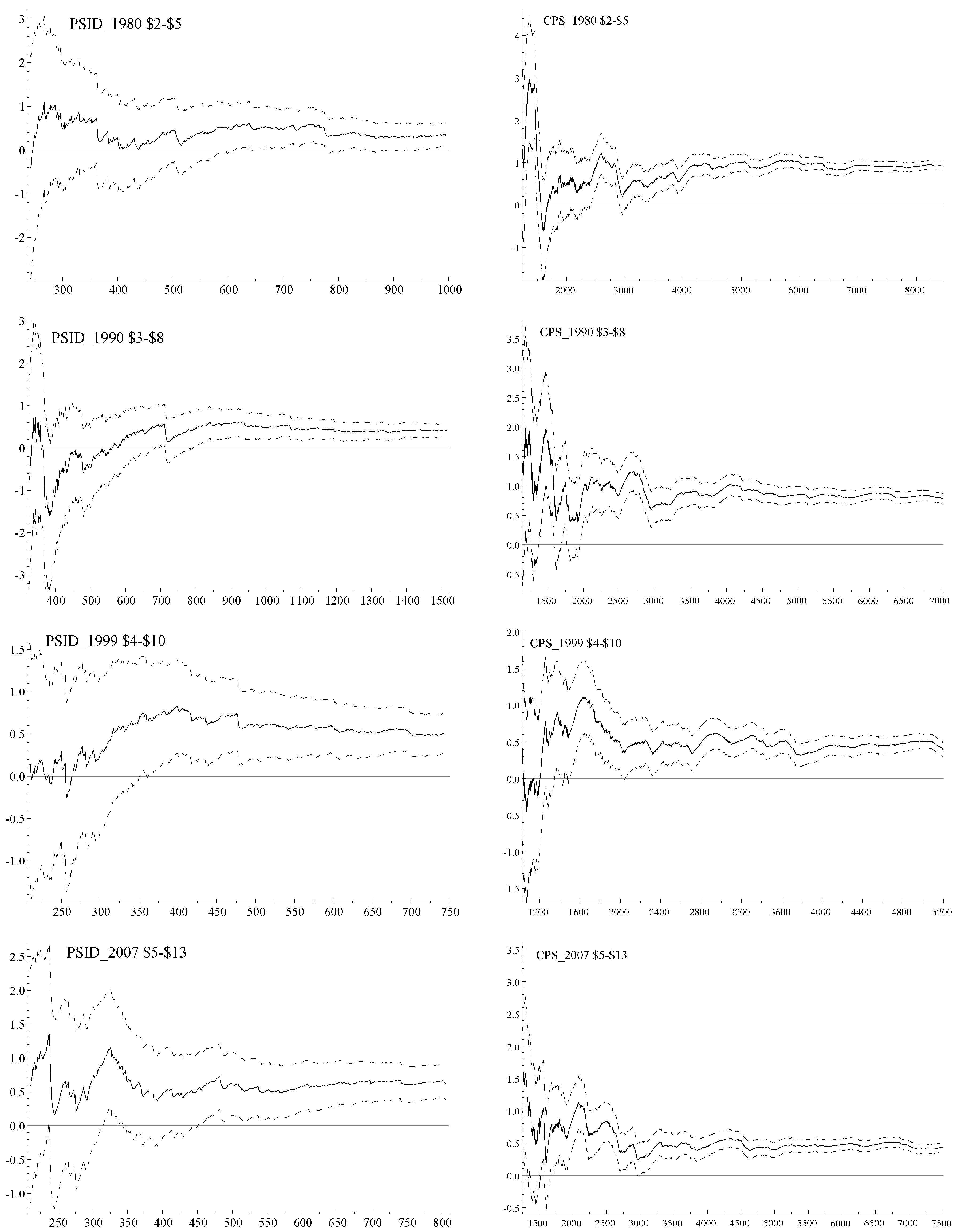
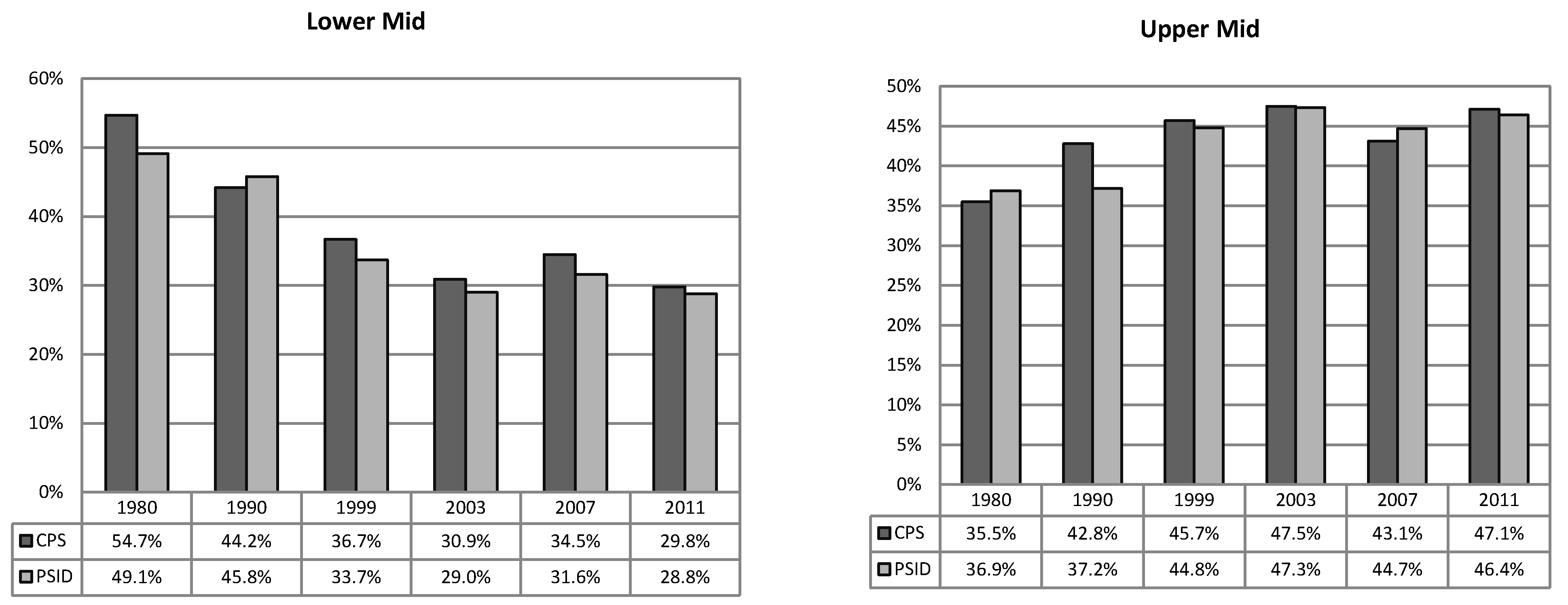
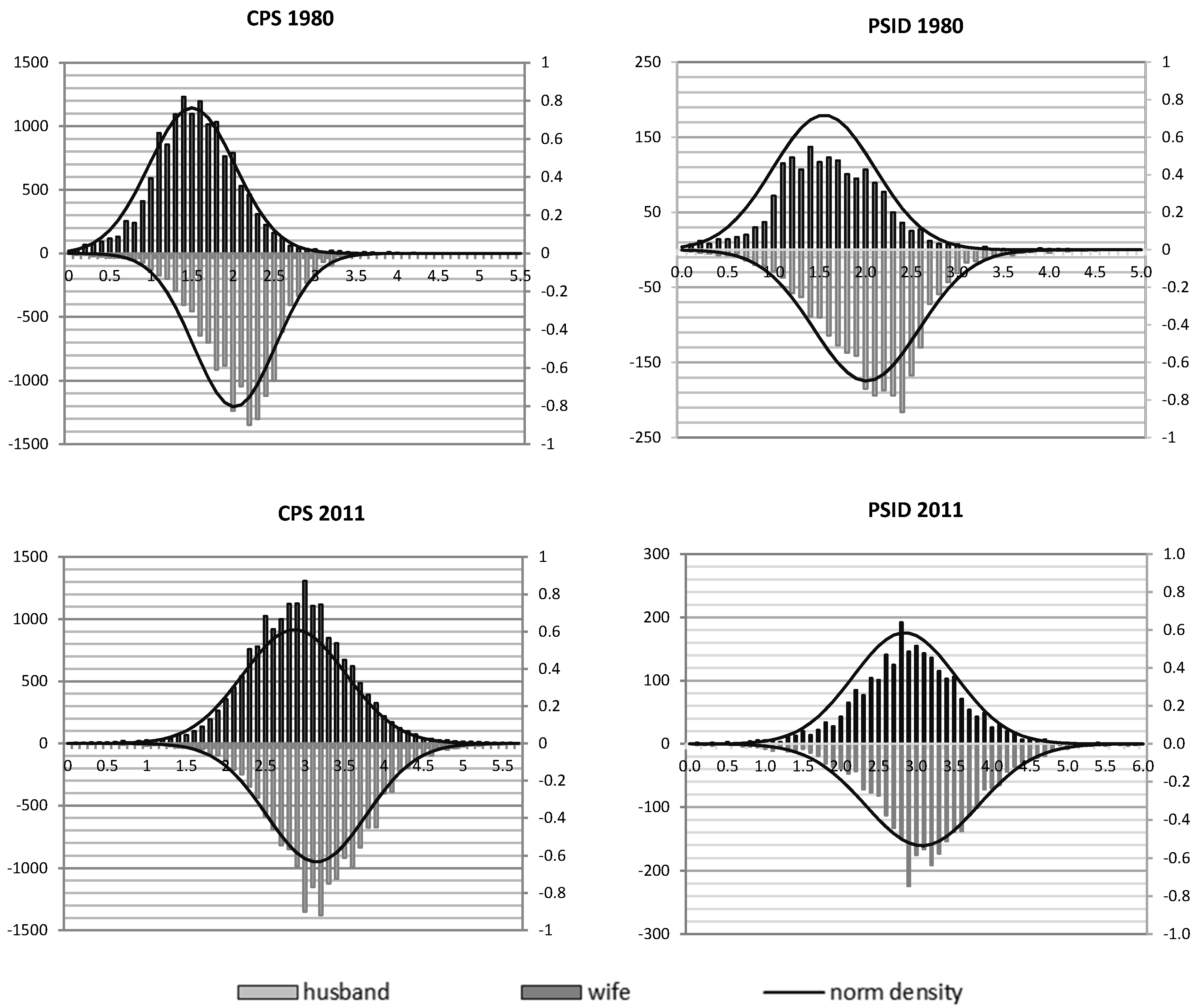