Interpretation and Semiparametric Efficiency in Quantile Regression under Misspecification

Abstract

Allowing for misspecification in the linear conditional quantile function, this paper provides a new interpretation and the semiparametric efficiency bound for the quantile regression parameter $\beta (\tau )$ in Koenker and Bassett (1978). The first result on interpretation shows that under a mean-squared loss function, the probability limit of the Koenker–Bassett estimator minimizes a weighted distribution approximation error, defined as $F_Y(X^{\prime }\beta (\tau )|X)-\tau$, i.e., the deviation of the conditional distribution function, evaluated at the linear quantile approximation, from the quantile level. The second result implies that the Koenker–Bassett estimator semiparametrically efficiently estimates the quantile regression parameter that produces parsimonious descriptive statistics for the conditional distribution. Therefore, quantile regression shares the attractive features of ordinary least squares: interpretability and semiparametric efficiency under misspecification.

1. Introduction

This paper revisits the approximation properties of the linear quantile regression under misspecification ([1,2,3]). The quantile regression estimator, introduced by the seminal paper of Koenker and Bassett [4], offers parsimonious summary statistics for the conditional quantile function and is computationally tractable. Since the development of the estimator, researchers have frequently used quantile regression, in conjunction with ordinary least squares regression, to analyse how the outcome variable responds to the explanatory variables. For example, to model wage structure in labour economics, Angrist, Chernozhukov, and Fernández-Val [1] study returns to education at different points in the wage distribution and changes in inequality over time. A thorough review of recent developments in quantile regression can be found in [5]. The object of interest of this paper is the quantile regression (QR) parameter that is the probability limit of the Koenker–Bassett estimator without assuming the true conditional quantile function to be linear. Two results are presented: a new interpretation and the semiparametric efficiency bound for the QR parameter.

The topic of interest is the conditional distribution function (CDF) of a continuous response variable Y given the regressor vector X, denoted as $F_Y(y|X)$. An alternative for the CDF is the conditional quantile function (CQF) of Y given X, defined as $Q_{\tau }(Y|X):=inf\{y:F_Y(y|X)\ge \tau \}$ for any quantile index $\tau \in (0,1)$. Assuming integrability, the CQF minimizes the check loss function

$$\begin{array}{c}\hfill Q_{\tau }(Y|X)\in arg\underset{q\in \mathcal{Q}}{\min }E\left[{\rho }_{\tau }(Y-q(X))\right],\end{array}$$

where $\mathcal{Q}$ is the set of measurable functions of X, ${\rho }_{\tau }(u)=u(\tau -{\mathbf{1}}_{\{u\le 0\}})$ is known as the check function and ${\mathbf{1}}_{\{·\}}$ is the indicator function. A linear approximation to the CQF is provided by the QR parameter $\beta (\tau )$, which solves the population minimization problem

$$\begin{array}{c}\hfill \beta (\tau ):=arg\underset{b\in R^d}{\min }E\left[{\rho }_{\tau }(Y-X^{\prime }b)\right]\end{array}$$

(1)

assuming the integrability and uniqueness of the solution, and d is the dimension of X. The QR parameter $\beta (\tau )$ provides a simple summary statistic for the CQF. The QR estimator introduced in [4] is the sample analogue

$$\begin{array}{c}\hfill \widehat{\beta }(\tau )\in arg\underset{b\in R^d}{\min }\frac{1}{n}\sum _{i=1}^n{\rho }_{\tau }(Y_i-X_i^{\prime }b)\end{array}$$

(2)

for the random sample $(Y_i,X_i^{\prime },i\le n)$ on the random variables $(Y,X^{\prime })$. By the equivalent first-order condition, this estimator $\widehat{\beta }(\tau )$ is also the generalized method of moments (GMM) estimator based on the unconditional moment restriction ([6,7])

$$\begin{array}{c}\hfill E[(\tau -{\mathbf{1}}_{\{Y\le X^{\prime }\beta (\tau )\}})X]=0.\end{array}$$

(3)

This paper focuses on the population QR parameter defined by (1) or equivalently (3).

If the CQF is modelled to be linear in the covariates $Q_{\tau }(Y|X)=X^{\prime }\beta (\tau )$ or $F_Y(X^{\prime }\beta (\tau )|X)=\tau$, the coefficient $\beta (\tau )$ satisfies the conditional moment restriction

$$\begin{array}{c}\hfill E[\tau -{\mathbf{1}}_{\{Y\le X^{\prime }\beta (\tau )\}}|X]=0\end{array}$$

(4)

almost surely. In the theoretical and applied econometrics literature, this linear QR model is often assumed to be correctly specified. Nevertheless, a well-known crossing problem arises: the CQF for different quantiles may cross at some values of X, except when $\beta (\tau )$ is the same for all τ. A logical monotone requirement is violated for $Q_{\tau }(Y|X)$ or its estimator to be weakly increasing in the probability index τ given X. The crossing problem for estimation could be treated by rearranging the estimator (for example, see [8] and the references therein.1). However, the crossing problem remains for the population CQF, suggesting that the linear QR model (4) is inherently misspecified. That is, there is no $\beta (\tau )\in R^d$ satisfying the conditional moment (4) almost surely. Therefore, the parameter of interest in this paper is the QR parameter $\beta (\tau )$ defined by (1) or (3) without the linear CQF assumption in (4). We can view $\beta (\tau )$ as the pseudo-true value of the linear QR model under misspecification. As the Koenker–Bassett QR estimator is widely used, it is important to understand the approximation nature of the estimand.

For the mean regression counterpart, ordinary least squares (OLS) consistently estimates the linear conditional expectation and minimizes mean-squared error loss for fitting the conditional expectation under misspecification. Chamberlain [9] proves the semiparametric efficiency of the OLS estimator, which provides additional justification for the widespread use of OLS. The attractive features of OLS, interpretability and semiparametric efficiency, under misspecification, motivate my investigation of parallel properties in QR. I study how this QR parameter approximates the CQF and the CDF and calculate its semiparametric efficiency bound.

The first contribution of this paper is on how $\beta (\tau )$ minimizes the distribution approximation error, defined by $F_Y(X^{\prime }\beta (\tau )|X)-\tau$, under a mean-squared loss function. The first-order condition (3) can be understood as the orthogonality condition of the covariates X and the distribution approximation error in the projection model. I show that the QR parameter $\beta (\tau )$ minimizes the mean-squared distribution approximation error, inversely weighted by the conditional density function $f_Y(X^{\prime }\beta (\tau )|X)$. Angrist, Chernozhukov, and Fernández-Val [1] (henceforth ACF) show that $\beta (\tau )$ minimizes the mean-squared quantile specification error, defined by $Q_{\tau }(Y|X)-X^{\prime }\beta (\tau )$, using a weight primarily determined by the conditional density. ACF’s study, as well as my own results, suggests that QR approximates the CQF more accurately at points with more observations, but the corresponding CDF evaluated at the approximated point $F_Y(X^{\prime }\beta (\tau )|X)$ is more distant from the targeted quantile level τ. This trade-off is controlled by the conditional density, which is distinct from OLS approximating the conditional mean, because the distribution and quantile functions are generally nonlinear operators. This observation is novel and increases the understanding of how the QR summarizes the outcome distribution. A numerical example in Figure 1 in Section 4 illustrates this finding.

The second result is the semiparametric efficiency bound of the $\beta (\tau )$. Chamberlain’s results in [9] on the mean regression based on differentiable moment restrictions cannot be applied to semiparametric efficiency for QR, due to the lack of moment function differentiability in (3). Although Ai and Chen [10] provide general results for sequential moment restrictions containing unknown functions, which could cover the quantile regression setting, I calculate the efficiency bound accommodating regularity conditions specifically for the QR parameter $\beta (\tau )$ using the method of Severini and Tripathi [11]. It follows that the misspecification-robust asymptotic variance of the QR estimator $\widehat{\beta }(\tau )$ in (2) attains this bound, which means no regular2 estimator for (3) has smaller asymptotic variance than $\widehat{\beta }(\tau )$. This result might be expected for an M-estimator, but, to my knowledge, the QR application has not been demonstrated and discussed rigorously in any publication. Furthermore, I calculate the efficiency bounds for jointly estimating QR parameters at a finite number of quantiles for both linear projection (3) and linear QR (4) models. Employing the widely-used method of Newey [12], Newey and Powell [13] find the semiparametric efficiency bound for $\beta (\tau )$ of the correctly-specified linear CQF in (4). Note that the efficiency bounds for (3) do not imply the bounds for (4); nor does the converse hold.

In Section 2, I discuss the interpretation of the misspecified QR model in terms of approximating the CDF and the CQF. The theorems for the semiparametric efficiency bounds are in Section 3. In Section 4, I discuss the parallel properties of QR and OLS. The paper is concluded by a review of some existing efficient estimators for linear projection model (3) and linear QR model (4).

2. Interpreting QR under Misspecification

Let Y be a continuous response variable and X be a $d\times 1$ regressor vector. The quantile-specific residual is defined as the distance between the response variable and the CQF, ${\epsilon }_{\tau }:=Y-Q_{\tau }(Y|X)$ with the conditional density $f_{{\epsilon }_{\tau }}(e|X)$ at ${\epsilon }_{\tau }=e$ or $f_Y(y|X)$ at $Y=y=e+Q_{\tau }(Y|X)$ for any $\tau \in (0,1)$. This is a semiparametric problem in the sense that the distribution functions of ${\epsilon }_{\tau }$ and X, as well as the CQF, are unspecified and unrestricted other than by the following assumptions, which are standard in QR models. I assume the following regularity conditions, based on the conditions of Theorem 3 in ACF.

(R1)

$(Y_i,X_i,i\le n)$ are independent and identically distributed on the probability space $(\Omega ,\mathcal{F},P)$ for each n;

(R2)

the conditional density $f_Y(y|X=x)$ exists and is bounded and uniformly continuous in y, uniformly in x over the support of X;

(R3)

$J(\tau ):=E\left[f_Y(X^{\prime }\beta (\tau )|X)X{X}^{\prime }\right]$ is positive definite for all $\tau \in (0,1)$, where $\beta (\tau )$ is uniquely defined in (1);

(R4)

${E\parallel X\parallel }^{2+ϵ}<\infty$ for some $ϵ>0$;

(R5)

$f_Y(X^{\prime }\beta (\tau )|X)$ to be bounded away from zero.

The identification of the pseudo-true parameter $\beta (\tau )$ is assumed in (R3). The bounded conditional density function of the continuous response variable Y given X in (R2) is needed for the existence of the CQF for any $\tau \in (0,1)$. The uniform continuity guarantees the existence and differentiability of the distribution function, i.e., $d{F}_Y(y|X)/dy=f_Y(y|X)$ and $F_Y(y|X)={\int }_{-\infty }^y{f}_Y(u|X)du$ with probability one. (R4) is used for the asymptotic normality of $\sqrt{n}(\widehat{\beta }(\tau )-\beta (\tau ))$. The covariates X are allowed to contain discrete components. (R5) guarantees that the objective function defined below in Equation (6) is finite $\forall \beta \in R^d$, where $\beta (\tau )$ is the parameter of interest uniquely defined by Equation (1).

The parameter of interest $\beta (\tau )$ is equivalent to solving

$$\begin{array}{c}\hfill E\left[X\left(F_Y\left(X^{\prime }\beta (\tau )|X\right)-\tau \right)\right]=0\end{array}$$

(5)

by applying the law of iterated expectations on Equation (3). Equation (5) states that X is orthogonal to the distribution approximation error $F_Y\left(X^{\prime }\beta (\tau )|X\right)-\tau$. The following theorem interprets QR via a weighed mean-squared error loss function on the distribution approximation error.

Theorem 1. 

Assume (R1)–(R5). Then, $\overline{\beta }(\tau )=\beta (\tau )$ solves the equation

$$\begin{array}{c}\hfill \overline{\beta }(\tau )=arg\underset{b\in R^d}{\min }E\left[{\left(f_Y(X^{\prime }\overline{\beta }(\tau )|X)\right)}^{-1}{\left(F_Y(X^{\prime }b|X)-\tau \right)}^2\right].\end{array}$$

(6)

Furthermore, if $E\left[\left(f_Y(X^{\prime }b|X)+(F_Y(X^{\prime }b|X)-\tau )f_Y^{\prime }(X^{\prime }b|X)/f_Y(X^{\prime }b|X)\right)X{X}^{\prime }\right]$ is positive definite at $b=\beta (\tau )$, then $\overline{\beta }(\tau )=\beta (\tau )$ is the unique solution to this problem (6).

Proof of Theorem 1. 

The objective function in (6) is finite by the assumptions. Any fixed point $b=\overline{\beta }(\tau )$ would solve the first-order condition, $E\left[X\left(F_Y\left(X^{\prime }b|X\right)-\tau \right)\right]=0$. By the law of iterated expectations, (3) implies the above first-order condition. Therefore, $\beta (\tau )$ solves (6). When the second-order condition holds, i.e., $E\left[\left(f_Y(X^{\prime }b|X)+(F_Y(X^{\prime }b|X)-\tau )f_Y^{\prime }(X^{\prime }b|X)/f_Y(X^{\prime }b|X)\right)X{X}^{\prime }\right]$ is positive definite at $b=\beta (\tau )$, $\beta (\tau )$ solves (6) uniquely.    ☐

Theorem 1 states that $\beta (\tau )$ is the unique fixed point to an iterated minimum distance approximation, with a weight of a function of X only. The mean-squared loss makes it clear how the linear function matches the CDF to the targeted probability of interest. The loss function puts more weight on points where the conditional density $f_Y(X^{\prime }\beta (\tau )|X)$ is small. As a result, the distribution approximation error is smaller at points with smaller conditional density.

Now, I discuss the approximation nature of QR based on the distributional approximation error and quantile specification error. ACF interpret QR as the minimizer of the weighted mean-squared error loss function for quantile specification error, defined as the deviation between the approximation point $X^{\prime }\beta (\tau )$ and the true CQF $Q_{\tau }(Y|X)$,3

$$\begin{array}{cc}\hfill \beta (\tau )& =arg\underset{\beta \in R^d}{\min }E\left[{\overline{w}}_{\tau }(X,\beta (\tau )){\left(X^{\prime }\beta -Q_{\tau }(Y|X)\right)}^2\right],\mathrm{where}\hfill \end{array}$$

(7)

$$\begin{array}{cc}\hfill {\overline{w}}_{\tau }(X,\beta (\tau ))& =\frac{1}{2}{\int }_0^1{f}_{{\epsilon }_{\tau }}\left(u\left(X^{\prime }\beta (\tau )-Q_{\tau }(Y|X)\right)|X\right)du.\hfill \end{array}$$

(8)

ACF define ${\overline{w}}_{\tau }(X,\beta (\tau ))$ in (8) to be the importance weights that are the averages of the response variable over a line connecting the approximation point $X^{\prime }\beta (\tau )$ and the true CQF. ACF note that the regressors contribute disproportionately to the QR estimate and the primary determinant of the importance weight is the conditional density.

Moreover, the first-order condition implied by (7) $E\left[{\overline{w}}_{\tau }(X,\beta (\tau ))X\left(X^{\prime }\beta (\tau )-Q_{\tau }(Y|X)\right)\right]=0$ is a weighted orthogonal condition of the quantile specification error. A Taylor expansion provides intuition to connect the distribution approximation error and the quantile specification error: ${\left(f_Y(X^{\prime }\beta |X)\right)}^{-1}{\left(F_Y(X^{\prime }\beta |X)-\tau \right)}^2\approx f_Y(X^{\prime }\beta |X){\left(Q_{\tau }(Y|X)-X^{\prime }\beta \right)}^2$ by $f_Y(X^{\prime }\beta |X)=f_{{\epsilon }_{\tau }}(X^{\prime }\beta -Q_{\tau }(Y|X)|X)$. This observation implies the quantile specification error is smaller at points where the conditional density $f_Y(X^{\prime }\beta |X)$ is larger. On the other hand, the distribution approximation error is larger at points with larger $f_Y(X^{\prime }\beta |X)$. Comparing with the OLS, where the mean operator is linear, the CDF and its inverse operator, the CQF, are generally nonlinear. The distribution approximation error can be interpreted as the distance after a nonlinear transformation by the CDF, $F_Y(X^{\prime }\beta (\tau )|X)-F_Y(Q_{\tau }(Y|X)|X)$. A Taylor expansion linearizes the distribution function to the quantile specification error multiplied by the conditional density function. The conditional density plays a crucial role on weighting the distribution approximation error and the quantile specification error. The above discussion provides additional insights to how the QR parameter approximates the CQF and fits the CDF to the targeted quantile level.

Remark 1 

(Mean-squared loss under misspecification). The linear function $X^{\prime }\beta (\tau )$ is the best linear approximation under the check loss function in (1). While $\beta (.5)$ is the least absolute derivations estimation, the QR parameter $\beta (\tau )$ for $\tau \ne 0.5$ is the best linear predictor for a response variable under the asymmetric loss function ${\rho }_{\tau }(·)$ in (1). ACF note that the prediction under the asymmetric check loss function is often not the object of interest in empirical work, with the exception of the forecasting literature, for example [15]. For the mean regression counterpart, OLS consistently estimates the linear conditional expectation and minimizes mean-squared error loss for fitting the conditional expectation under misspecification. The robust nature of OLS also motivates research on misspecification in panel data models. For example, Galvao and Kato [16] investigate linear panel data models under misspecification. The pseudo-true value of the fixed effect estimator provides the best partial linear approximation to the conditional mean given the explanatory variables and the unobservable individual effect.4

3. The Semiparametric Efficiency Bounds

Section 3.1 presents the semiparametric efficiency bound for the unconditional moment restriction (3). Section 3.2 discusses the existing results on the semiparametric efficiency bound for the conditional moment restriction (4).

3.1. QR under Misspecification

I calculate the semiparametric efficiency bound for the unconditional moment restriction (3) by the approach of Severini and Tripathi [11].

Theorem 2. 

Assume (R1)–(R4). The semiparametric efficiency bound for estimating the population QR parameter $\beta (\tau )$, defined in (1) or equivalently (3), is $J{(\tau )}^{-1}\Gamma (\tau ,\tau )J{(\tau )}^{-1}$, where $J(\tau )$ is defined in (R3) and

$$\begin{array}{c}\hfill \Gamma ({\tau }_i,{\tau }_j):=E\left[\left({\tau }_i-{\mathbf{1}}_{\{Y<X^{\prime }\beta ({\tau }_i)\}}\right)\left({\tau }_j-{\mathbf{1}}_{\{Y<X^{\prime }\beta ({\tau }_j)\}}\right)X{X}^{\prime }\right]\end{array}$$

for any ${\tau }_i,{\tau }_j\in \mathcal{T}:=$ a closed subset of $[ϵ,1-ϵ]$ for $ϵ>0$.

In general, the semiparametrically-efficient joint asymptotic covariance of the estimators for $({\beta }^{\prime }({\tau }_1),{\beta }^{\prime }({\tau }_2),...,{\beta }^{\prime }{({\tau }_m)}^{\prime }$ is $J{({\tau }_i)}^{-1}\Gamma ({\tau }_i,{\tau }_j)J{({\tau }_j)}^{-1}$, for any ${\tau }_i,{\tau }_j\in \mathcal{T}$, $i,j=1,2,...,m$, for a finite integer $m\ge 1$.

Proof of Theorem 2. 

See the Appendix.    ☐

My proof accommodates the regularity assumptions for quantile regression and modifies Section 9 of [11]. For example, the covariate X can contain discrete components, by constructing two tangent spaces for the conditional density of Y given X and the marginal density of X, respectively. In the efficiency bound, $J(\tau ):=E\left[f_Y(X^{\prime }\beta (\tau )|X)X{X}^{\prime }\right]$ is obtained by assuming the interchangeability of integration and differentiation for the nonsmooth check function.5

The method in [11] has been used in the monotone binary model in [18], Lewbel [19] latent variable model in [20] and the partial linear single index model in [21], for example. I work in the Hilbert space of tangent vectors of the square-root density functions and using the Riesz–Fréchet representation theorem. Another equivalent approach in [12] works in a Hilbert space of random variables and uses the projection on the linear space spanned by the scores from the one-dimensional subproblems to find the efficient influence function. The efficiency bound is then the second moment of the efficient influence function, $J{(\tau )}^{-1}X(\tau -{\mathbf{1}}_{\{Y\le X^{\prime }\beta \}})$. Newey’s efficient influence function is the score function evaluated at the unique representers by the Riesz–Fréchet theorem used in [11]; a more detailed comparison of these two approaches is discussed in [11].

ACF show that the QR process $\widehat{\beta }(·)$ is asymptotically mean-zero Gaussian with the covariance function $J{({\tau }_1)}^{-1}\Gamma ({\tau }_1,{\tau }_2)J{({\tau }_2)}^{-1}$ for any ${\tau }_1,{\tau }_2\in \mathcal{T}$, which is the semiparametric efficiency bound in Theorem 2. This asymptotic covariance under misspecification for a single quantile, $J{(\tau )}^{-1}\Gamma (\tau ,\tau )J{(\tau )}^{-1}$, has been presented in [2] and [3]. Hahn [3] further shows the QR estimator is well approximated by the bootstrap distribution, even when the linear quantile restriction is misspecified. An alternative estimator for the misspecification-robust asymptotic covariance matrix of $\widehat{\beta }(\tau )$ is the nonparametric kernel method in ACF.

3.2. QR for Linear Specification

Assuming the linear QR model in (4) is correctly specified, i.e., $Q_{\tau }(Y|X)=X^{\prime }\beta (\tau )$ almost surely, the asymptotic covariance for the QR process $\widehat{\beta }(·)$ derived by ACF is simplified to $J{({\tau }_1)}^{-1}{\Gamma }_0({\tau }_1,{\tau }_2)J{({\tau }_2)}^{-1}$, where ${\Gamma }_0({\tau }_1,{\tau }_2):=\left(\min \left\{{\tau }_1,{\tau }_2\right\}-{\tau }_1{\tau }_2\right)E[X{X}^{\prime }]$ for any ${\tau }_1,{\tau }_2\in (0,1)$. The asymptotic covariance $J{(\tau )}^{-1}{\Gamma }_0(\tau ,\tau )J{(\tau )}^{-1}$ for a single quantile τ, first derived by Powell [7], is widely used for inference in most empirical studies, which implicitly assume correct specification.

The semiparametric efficiency bound for the correctly-specified quantile regression (4) is $\tau (1-\tau ){\left(E\left[X{X}^{\prime }{f}_{{\epsilon }_{\tau }}^2(0|X)\right]\right)}^{-1}$, where $f_Y(X^{\prime }\beta (\tau )|X)=f_{{\epsilon }_{\tau }}(0|X)$ a.s. and $E\left[X{X}^{\prime }{f}_{{\epsilon }_{\tau }}^2(0|X)\right]$ is assumed to be finite and nonsingular. This is first calculated in [13] using the method developed in [12]. If, in addition, the conditional density function of ${\epsilon }_{\tau }$ given X is independent of X, i.e., $f_Y(Q_{\tau }(Y|X)|X)=f_{{\epsilon }_{\tau }}(0|X)=f_{{\epsilon }_{\tau }}(0)$, and $f_{{\epsilon }_{\tau }}(0)>0$, the semiparametric efficiency bound becomes $\tau (1-\tau ){\left(E[X{X}^{\prime }]\right)}^{-1}/f_{{\epsilon }_{\tau }}^2(0)$. This asymptotic covariance is attained by $\widehat{\beta }(\tau )$, first shown in [4]. This has an interesting resemblance to the fact that the OLS estimator is semiparametrically efficient in a homoskedastic regression model, i.e., $e=Y-X^{\prime }\beta$, $E[e|X]=0$, and $E[e^2|X]=E[e^2]$.

I further show, in general, that the semiparametrically-efficient joint asymptotic covariance of the estimators for ${({\beta }^{\prime }({\tau }_1),...,{\beta }^{\prime }({\tau }_m))}^{\prime }$ is

$$\begin{array}{c}\hfill \left(\min \left\{{\tau }_i,{\tau }_j\right\}-{\tau }_i{\tau }_j\right){\left(E\left[X{X}^{\prime }{f}_{{\epsilon }_{{\tau }_i}}(0|X)f_{{\epsilon }_{{\tau }_j}}(0|X)\right]\right)}^{-1}\end{array}$$

(9)

for any ${\tau }_i,{\tau }_j\in \mathcal{T}$, $i,j=1,2,...,m$, for any finite integer $m\ge 1$. The regularity conditions imposed, (R1), (R2) and (R4), are weaker than the assumptions in [13]; for example, they assume $f(\epsilon ,X)$ is absolutely continuous in ε, which implies uniform continuity in (R2). See the Appendix for the detailed proof for (9).

4. Discussion and Conclusions

Misspecification is a generic phenomenon; especially in quantile regression (QR), the true conditional quantile function (CQF) might be nonlinear or different functions of the covariates at different quantiles. Table 1 summarizes the parallel properties of QR and OLS. Under misspecification, the pseudo-true OLS coefficient can be interpreted as the best linear predictor of the conditional mean function, $E[Y|X]$, in the sense that the coefficient minimizes the mean-squared error of the linear approximation to the conditional mean. The approximation properties of OLS have been well studied (see, for example, [22]). With respect to the QR counterpart, I present the inverse density-weighted mean-squared error loss function based on the distribution approximation error $F_Y(X^{\prime }\beta |X)-\tau$. This result complements the interpretation based on the quantile specification error in [1]. My results imply that the Koenker–Bassett estimator is semiparametrically efficient for misspecified linear projection models and correctly specified linear quantile regression models when $f_Y(Q_{\tau }(Y|X)|X)=f_{{\epsilon }_{\tau }}(0|X)$ does not depend on X. Alternatively, the smoothed empirical likelihood estimator using the unconditional moment restriction in [23] has the same asymptotic distribution as the Koenker-Bassett estimator and, hence, attains the efficiency bound.

Table 1. Summary properties of OLS and quantile regression (QR).

	OLS	QR
	Linear Projection Model
objective minimized	$E[{(Y-X^{\prime }\beta )}^2]$	$E[{\rho }_{\tau }(Y-X^{\prime }\beta (\tau ))]$
(interpretation)	$E[{(E[Y|X]-X^{\prime }\beta )}^2]$	$E[{\overline{w}}_{\tau }{(Q_{\tau }(Y|X)-X^{\prime }\beta (\tau ))}^2]$
		$E[f_Y{(X^{\prime }\beta (\tau )|X)}^{-1}{(F_Y(X^{\prime }\beta (\tau )|X)-\tau )}^2]$
unconditional moment	$E[X(Y-X^{\prime }\beta )]=0$	$E[X({\mathbf{1}}_{\{Y\le X^{\prime }\beta (\tau )\}}-\tau )]=0$
(interpretation)	$E[X(E[Y|X]-X^{\prime }\beta )]=0$	$E[X(F_Y(X^{\prime }\beta (\tau )|X)-\tau )]=0$
		$E\left[{\overline{w}}_{\tau }X\left(X^{\prime }\beta (\tau )-Q_{\tau }(Y|X)\right)\right]=0$
efficient estimators	$arg{\min }_{\beta \in R^d}\frac{1}{n}{\sum }_{i=1}^n{(Y_i-X_i^{\prime }\beta )}^2$	$arg{\min }_{\beta \in R^d}\frac{1}{n}{\sum }_{i=1}^n{\rho }_{\tau }(Y_i-X_i^{\prime }\beta )$
	$={({\sum }_{i=1}^n{X}_i{X}_i^{\prime })}^{-1}({\sum }_{i=1}^n{X}_i{Y}_i)$	(Koenker–Bassett)
	(OLS)
asymptotic covariance	$Q^{-1}\Omega Q^{-1}$ ${}^{*}$	$J^{-1}\Gamma J^{-1}$
efficiency bounds	Chamberlain (1987) [9]	Theorem 2
	Linear Regression Model
conditional moment	$E[Y|X]=X^{\prime }\beta$	$Q_{\tau }(Y|X)=X^{\prime }\beta (\tau )$
		or $F_Y(X^{\prime }\beta (\tau )|X)=\tau$
efficiency bounds	Chamberlain (1987) [9] ${}^{†}$	Newey and Powell (1990) [13]
homoscedasticity-type	$var[Y|X]={\sigma }^2$	$f_{{\epsilon }_{\tau }}(0|X)=f_{{\epsilon }_{\tau }}(0)$
condition
efficient estimators	OLS	Koenker–Bassett

${}^{*}$ $Q=E[X{X}^{\prime }]$ and $\Omega =E[X{X}^{\prime }{e}^2]$ where $e=Y-X^{\prime }\beta$; ${}^{†}$ The feasible generalized least squares estimator is semiparametrically efficient, for example.

Table 1. Summary properties of OLS and quantile regression (QR).

	OLS	QR
	Linear Projection Model
objective minimized	$E[{(Y-X^{\prime }\beta )}^2]$	$E[{\rho }_{\tau }(Y-X^{\prime }\beta (\tau ))]$
(interpretation)	$E[{(E[Y|X]-X^{\prime }\beta )}^2]$	$E[{\overline{w}}_{\tau }{(Q_{\tau }(Y|X)-X^{\prime }\beta (\tau ))}^2]$
		$E[f_Y{(X^{\prime }\beta (\tau )|X)}^{-1}{(F_Y(X^{\prime }\beta (\tau )|X)-\tau )}^2]$
unconditional moment	$E[X(Y-X^{\prime }\beta )]=0$	$E[X({\mathbf{1}}_{\{Y\le X^{\prime }\beta (\tau )\}}-\tau )]=0$
(interpretation)	$E[X(E[Y|X]-X^{\prime }\beta )]=0$	$E[X(F_Y(X^{\prime }\beta (\tau )|X)-\tau )]=0$
		$E\left[{\overline{w}}_{\tau }X\left(X^{\prime }\beta (\tau )-Q_{\tau }(Y|X)\right)\right]=0$
efficient estimators	$arg{\min }_{\beta \in R^d}\frac{1}{n}{\sum }_{i=1}^n{(Y_i-X_i^{\prime }\beta )}^2$	$arg{\min }_{\beta \in R^d}\frac{1}{n}{\sum }_{i=1}^n{\rho }_{\tau }(Y_i-X_i^{\prime }\beta )$
	$={({\sum }_{i=1}^n{X}_i{X}_i^{\prime })}^{-1}({\sum }_{i=1}^n{X}_i{Y}_i)$	(Koenker–Bassett)
	(OLS)
asymptotic covariance	$Q^{-1}\Omega Q^{-1}$ ${}^{*}$	$J^{-1}\Gamma J^{-1}$
efficiency bounds	Chamberlain (1987) [9]	Theorem 2
	Linear Regression Model
conditional moment	$E[Y|X]=X^{\prime }\beta$	$Q_{\tau }(Y|X)=X^{\prime }\beta (\tau )$
		or $F_Y(X^{\prime }\beta (\tau )|X)=\tau$
efficiency bounds	Chamberlain (1987) [9] ${}^{†}$	Newey and Powell (1990) [13]
homoscedasticity-type	$var[Y|X]={\sigma }^2$	$f_{{\epsilon }_{\tau }}(0|X)=f_{{\epsilon }_{\tau }}(0)$
condition
efficient estimators	OLS	Koenker–Bassett

${}^{*}$ $Q=E[X{X}^{\prime }]$ and $\Omega =E[X{X}^{\prime }{e}^2]$ where $e=Y-X^{\prime }\beta$; ${}^{†}$ The feasible generalized least squares estimator is semiparametrically efficient, for example.

Under the linear quantile regression model, the Koenker–Bassett estimator consistently estimates the true $\beta (\tau )$, although it is not semiparametrically efficient given heteroskedasticity. Researchers have proposed many efficient estimators for the correctly-specified linear quantile regression parameter, for example the one-step score estimator in [13], the smoothed conditional empirical likelihood estimator in [24] and the sieve minimum distance (SMD) estimator in [25,26]. However, for all of these estimators, the pseudo-true values under misspecification are different, and their interpretations have not been thoroughly studied. Therefore, the semiparametric efficiency bounds of these pseudo-true values are also different. For example, an unweighted SMD estimator converges to a pseudo-true value ${\beta }_{SMD}$ that minimizes $E\left[{\left(F_Y(X^{\prime }\beta |X)-\tau \right)}^2\right]$.6 The first-order condition is $E\left[X\left(F_Y(X^{\prime }{\beta }_{SMD}|X)-\tau \right)f_Y(X^{\prime }{\beta }_{SMD}|X)\right]=0$, which is the unconditional moment used in [13] for the semiparametrically efficient GMM estimator under correct specification. The conditional density weight is similar to the generalized least squares in the mean regression in that it uses a weight function of the conditional variance to construct an efficient estimator.

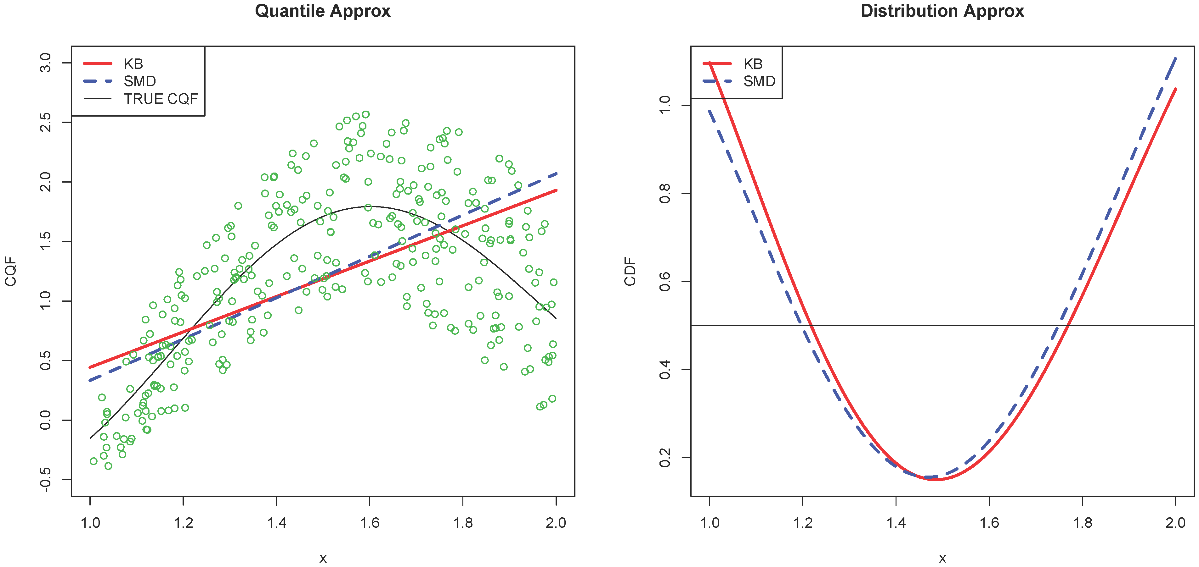
It is interesting to note that the pseudo-true value of the SMD estimator minimizes $E\left[{\left(F_Y(X^{\prime }\beta |X)-\tau \right)}^2\right]\approx E\left[f_Y^2(Q_{\tau }(Y|X)|X){\left(X^{\prime }\beta -Q_{\tau }(Y|X)\right)}^2\right]$. The distribution approximation error is weighted evenly over the support of X for ${\beta }_{SMD}$, in contrast to the QR parameter, which is weighted more at points with smaller conditional density in Theorem 1. Therefore, the SMD estimator might have more desirable and reasonable approximation properties than QR. Nevertheless, the SMD estimator is computationally more demanding than the Koenker–Bassett estimator. A numerical example in Figure 1 illustrates how the Koenker and Bassett (KB) and SMD estimators approximate the CQF and the CDF.

Figure 1. This numerical example is constructed by $X\sim Uniform[1,2]$, $e|X=x\sim Uniform[0,x]$ and $Y=cos(2X)+e$. Therefore, $f_Y(y|X)=1/X$, $F_Y(y|X)=(y-cos(2X))/X$ and $Q_{\tau }(Y|X)=\tau X+cos(4X)$. Set $\tau =0.5$ for the median. The red solid line is for the QR parameter ${\beta }_{KB}$ defined in (3) and estimated by the Koenker-Bassett (KB) estimator. The blue dashed line is the approximation by the SMD estimator ${\beta }_{SMD}$ minimizing $E[{(F_Y(X^{\prime }\beta |X)-\tau )}^2]$. The approximations are $X^{\prime }{\beta }_{KB}=-0.324+0.161X$ and $X^{\prime }{\beta }_{SMD}=-0.204+0.078X$. The left panel shows the linear approximations $X^{\prime }{\beta }_{KB}$, $X^{\prime }{\beta }_{SMD}$ and the true CQF. The green circles are 300 random draws from the DGP. The right panel shows the corresponding CDFs $F_Y(X^{\prime }{\beta }_{KB}|X)$ and $F_Y(X^{\prime }{\beta }_{SMD}|X)$. For smaller x where the conditional density is larger, the quantile specification error of SMD is smaller than that of KB in the left panel. For the distribution approximation error in the right panel, SMD weights more evenly over the support of X, while KB has smaller distribution approximation error at larger x with smaller density.

This discussion leads to open-ended questions: What is an appropriate linear approximation or a meaningful summary statistic for the nonlinear CQF? How should economists measure the marginal effect of the covariates on the CQF? An approach that circumvents this problem is measuring the average marginal response of the covariates on the CQF directly. The average quantile derivative, defined as $E[W(X)\nabla Q_{\tau }(Y|X)]$ where $W(X)$ is a weight function, offers such a succinct summary statistic ([27]). Sasaki [28] investigates the question that quantile regressions may misspecify true structural functions. He provides a causal interpretation of the derivative of the CQF, which identifies a weighted average of heterogeneous structural partial effects among the subpopulation of individuals at the conditional quantile of interest. Sasaki’s work adds economic content to this misspecified question. This paper complements the prior literature on understanding how the QR statistically summarizes the outcome distribution.