A Fast, Accurate Method for Value-at-Risk and Expected Shortfall

Abstract

A fast method is developed for value-at-risk and expected shortfall prediction for univariate asset return time series exhibiting leptokurtosis, asymmetry and conditional heteroskedasticity. It is based on a GARCH-type process driven by noncentral t innovations. While the method involves the use of several shortcuts for speed, it performs admirably in terms of accuracy and actually outperforms highly competitive models. Most remarkably, this is the case also for sample sizes as small as 250.

1. Introduction

Value-at-risk (VaR) and, more recently, expected shortfall (ES) are fundamental risk measures. In May 2012, the Basel Committee on Banking Supervision announced its intention to replace VaR with ES in banks’ internal models for determining regulatory capital requirements ([1] p. 3). Calculation of the ES requires first calculating the VaR, so that accurate methods for VaR are still necessary. Numerous papers have proposed and tested models for VaR prediction, which amounts to delivering a prediction of a left-tail quantile of the h-step ahead predictive distribution of a univariate time series of financial asset returns. Kuester et al. [2] discuss and compare numerous models and show that competitive models include the normal-mixture-GARCH type of models and GARCH-type models driven by heavy-tailed, asymmetric innovations (in this case, we use the noncentral t distribution, or NCT-GARCH).

In this paper, we develop an extremely fast method for VaR and ES prediction based on NCT-GARCH and demonstrate its viability. We use two variants of the normal-mixture-GARCH model class as a benchmark for testing, given its outstanding prediction performance, as demonstrated in Kuester et al. [2] and Haas et al. [3]. Unfortunately, the method we employ to speed up the NCT-GARCH estimation is not straightforwardly applicable to the normal-mixture-GARCH framework, and so, the latter is, relative to our newly proposed technique, extremely slow.

There are at least two reasons for developing a fast (and accurate) method for VaR and ES prediction. The first is that large financial institutions are required to compute and report VaR (and soon, perhaps, the ES) of customer portfolios. With the potential number of clients in the tens of thousands, speed (and accuracy) are crucial. The second reason is that the method can then be used in a portfolio optimization framework, in which the ES values corresponding to thousands of candidate portfolios need to be computed.

The rest of this paper is organized as follows. Section 2 develops the methodology for computing the NCT-APARCHmodel in a fraction of the time otherwise required by standard maximum likelihood methods. Section 3 presents an extensive forecast comparison revealing the usefulness of the new approach in terms of density and VaR forecasting. Section 4 concludes.

2. NCT-GARCH

With respect to the class of GARCH-type models driven by heavy-tailed, asymmetric innovations, we consider an APARCH model driven by innovations from a (singly) noncentral t distribution, hereafter NCT. While there are several ways of introducing asymmetry into the Student’s t distribution, the benefit of this choice is that the NCT is closed under addition, in the sense that sums of margins of the Kshirsagar [4] multivariate NCT is again NCT (see, e.g., [5]), so that, if the set of asset returns is modeled using a multivariate NCT, then the portfolio distribution is analytically tractable; see, e.g., Jondeau [6] and Broda et al. [7]. The idea of using the (univariate) NCT distribution for modeling asset returns goes back to Harvey and Siddique [8].

Section 2.1 introduces the model and discusses computational aspects and problems concerning the NCT density and expressions for VaR and ES. Section 2.2 revives the idea of using fixed, instead of estimated, GARCH parameters and details the idea of how to construct a fast and accurate estimator for the NCT-APARCH model, with a location parameter. Section 2.2.1 introduces a new approach to estimating the location coefficient, which is extremely fast and nearly as accurate as the use of the maximum likelihood estimator (MLE). Section 2.2.2 shows the calibration of the GARCH parameters, and Section 2.2.3 focuses on the subsequent parameter fixing of the APARCH asymmetry parameter. In Section 2.3, the use of a lookup table, based on sample and theoretical quantiles, is developed. This is shown to be virtually as accurate as maximum likelihood estimation, but far faster.

2.1. Model

With a GARCH structure, the model is:

$$R_t=a_0+Z_t^{*}{\sigma }_t,Z_t^{*}=Z_t-\mu ,Z_t\stackrel{\mathrm{iid}}{\sim }NCT(k,\gamma )$$

(1)

with:

$$\mu =\mathbb{E}\left[Z_t\right]={\left(\frac{k}{2}\right)}^{1/2}\frac{\Gamma \left(k/2-1/2\right)}{\Gamma \left(k/2\right)}\gamma$$

$k\in {\mathbb{R}}_{>0}$ is the degrees of freedom, and $\gamma \in \mathbb{R}$ is the noncentrality parameter, which dictates the asymmetry; see, e.g., Paolella [9], Section 10.4, for details on computing the density and cumulative distribution function (cdf) of the (singly and doubly) NCT using exact and saddle point methods. The evolution of the scale parameter ${\sigma }_t$ can be modeled rather flexibly by the APARCH model proposed by Ding et al. [10], given by:

$${\sigma }_t^{\delta }=c_0+\sum _{i=1}^r{c}_i{\left(\left|{ϵ}_{t-i}\right|-{\gamma }_i{ϵ}_{t-i}\right)}^{\delta }+\sum _{i=1}^s{d}_i{\sigma }_{t-i}^{\delta },{ϵ}_t=Z_t^{*}{\sigma }_t$$

(2)

with $c_i>0$, $d_i\ge 0$, $\delta >0$ and $\left|{\gamma }_i\right|<1$. Calculations show that the likelihood is often relatively flat in δ for values between one and two, so we just set $\delta =2$, as well as taking the usual values of $r=s=1$. We will investigate the effect of varying asymmetry parameter ${\gamma }_1$ below in Section 2.2.3 and first take it to be zero for the development of the fast estimation method. Note that the structure of Equation (2) implies that ${\sigma }_t$ is independent of $Z_t^{*}$, so that, in Equation (1), $\mathbb{E}\left[R_{P,t}\right]=a_0$, a result we require below.

The major potential drawback of this model is that, using conventional constructs, the likelihood is very slow to compute: The NCT density can be expressed as an infinite sum,

$$\begin{array}{cc}\hfill f_Z\left(t;k,\gamma \right)& ={\text{e}}^{-{\gamma }^2/2}\frac{\Gamma \left(\left(k+1\right)/2\right)k^{k/2}}{\sqrt{\pi }\Gamma \left(k/2\right)}{\left(\frac{1}{k+t^2}\right)}^{\frac{k+1}{2}}\hfill \\ & \times \left[\sum _{i=0}^{\infty }\frac{{\left(t\gamma \right)}^i}{i!}{\left(\frac{2}{t^2+k}\right)}^{i/2}\frac{\Gamma \left\{\left(k+i+1\right)/2\right\}}{\Gamma \left\{\left(k+1\right)/2\right\}}\right]\hfill \end{array}$$

(3)

as is used, for example, in MATLAB’s function, nctpdf.

Given that the likelihood entails computing the density at each point in the return series, and we envision this being done for thousands of such series, the use of Equation (3) will be prohibitive. This bottleneck was overcome by Broda and Paolella [11], in which a highly accurate saddle point approximation, hereafter SPA, was developed for the singly (and doubly) noncentral t distribution. The enormous speed increase is attained because: (i) the SPA equation can be explicitly solved, and thus, the evaluation of the approximation entails a small and fixed number of floating point operations; and (ii) the procedure can be “vectorized” in MATLAB and other vector-based computing languages. The SPA density needs to be renormalized to integrate to one, and this degrades its speed somewhat. However, a lookup table (based on a tight grid of the two parameter values) can be used to obviate the integration.

An alternative to the SPA, which is nearly as fast, but more accurate, is to use a simple, two-fold approximation to Equation (3). This is detailed in Appendix A.

From the fitted model and the h-step ahead density forecast, the VaR and ES are calculated. Calculation of quantiles requires root searching using the cdf, which also can be expressed as an infinite sum. However, the SPA can be used for the cdf, as well, as detailed in Broda and Paolella [11], so that the VaR is obtained in a fraction of the time otherwise required. The ES could be computed as follows: assuming the density of random variable X is continuous, the ES can be expressed via the tail conditional expectation, for a given confidence level $q\in (0,1)$, as:

$${\mathrm{ES}}^{\left(q\right)}\left(X\right)\equiv -\mathbb{E}\left[X\mid X\le -x_q\right]=-\frac{1}{q}{\int }_{-\infty }^{-x_q}u{f}_X\left(u\right)\text{d}u$$

(4)

where $x_q$ is the corresponding VaR (the negative 100q% quantile of X).

See Broda and Paolella [12] for further details on computing ES for various distributions popular in finance and Nadarajah et al. [13] for an overview and literature survey of ES and its estimation methods. The integral in Equation (4) can be evaluated using Equation (3) or, much faster, using the SPA density approximation. However, a yet much faster way is presented in Broda and Paolella [14], again via the use of saddle point methods, which completely avoids numeric integration and is shown to be highly accurate.

While the use of the SPA for the cdf and the ES enable much faster calculation of the VaR and ES, there is yet a faster way. That is to use a lookup table procedure. When using a closely spaced grid of values of k and $\gamma$, the delivered values of VaR and ES (for $2\le k\le 30$ and $-1\le \gamma \le 1$) are accurate to at least three significant digits. For building lookup tables, we employ the NCT density approximation in Appendix A, hereafter FastNCT.

2.2. Faster Estimation Method

Via the use of the SPA to the density of the NCT distribution, or by virtue of FastNCT, ML estimation of the NCT-APARCH model does not require much more time than the estimation of the usual t-GARCH model of Bollerslev [15]. Nevertheless, this method still entails joint optimization of at least five parameters and requires running the GARCH filter through the data at each iteration. As such, we propose an alternative method of estimation that is much faster. The core idea is to fix the APARCH parameters in advance, choosing a typical set of values associated with daily financial returns data. (This idea is of course not new and goes back at least to the RiskMetrics Technical Document of 1994, in which they essentially propose an integrated GARCH(1,1) model with $d_1=0.94$.) For the estimation of intercept parameter $a_0$ in Equation (1), as $\mathbb{E}\left[R_t\right]=a_0$, we use (in light of the heavy tails) a trimmed mean, as discussed below. The chosen GARCH filter is then applied to the location-centered returns $R_t-{\widehat{a}}_0$, yielding a (presumed) set of i.i.d. location-zero, scale-one NCT residuals.

Then, based on these residuals, one option is to compute the MLE of the two NCT density parameters. This procedure is between seven and 15 times faster than computing the MLE of the full model when using SPA or FastNCT (the time increase depending on the data set; presumably, the larger the degrees of freedom parameter, the longer estimation takes, because of a flatter likelihood). Another option, which is much faster and ultimately what we use and recommend, is to use a lookup table procedure based on sample quantiles. This is detailed below in Section 2.3.

The next two subsections consider: (i) the estimation of the location term $a_0$ assuming volatility-adjusted returns; and (ii) the motivation and justification of fixing the APARCH parameters.

2.2.1. Location Term $a_0$

We desire a very fast method for the estimation of $a_0$, which is still accurate. This is because the estimation error in the means of the returns are more consequential in asset allocation than those in the variance and covariance terms (see [16]). One could just take the sample mean, but given the potentially heavy tails of the data, this will be a poor choice. The median is also too extreme, especially after GARCH effects are accounted for. Consider the trimmed mean for a set of data $\mathbf{X}=(X_1,\cdots ,X_n)$, denoted $trim(\mathbf{X},\alpha )={\overline{X}}_{\left(\alpha \right)}$, $0\le \alpha <100$, computed as the mean of the $X_i$ after dropping the smallest and largest $\alpha /2\%$ of the sample. We wish to determine the optimal trimming value α, as a function of the degrees of freedom parameter k. Given that the fat tailed nature of asset returns is far more prominent than the asymmetry, we consider determining the optimal α just based on the usual Student’s t, i.e., $\gamma =0$. Let $X_i\stackrel{\mathrm{iid}}{\sim }t\left(k,\mu ,1\right)$, i.e., the Student’s t with degrees of freedom parameter k, location μ and scale one.

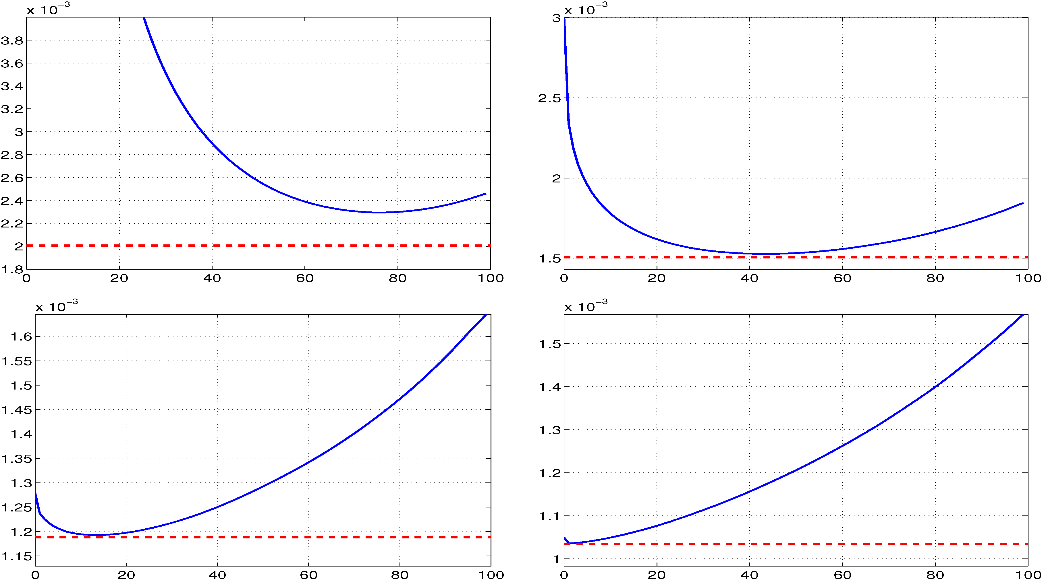
For a fixed k and based on a sample size of $n=1000$ (and, with no loss of generality, taking $\mu =0$), we simulate $s=50,000$ samples, and for each, ${\overline{X}}_{\left(\alpha \right)}$ was computed for each integer value of α ranging from zero to 99. For each α, the mean squared error (MSE) is approximated as $s^{-1}{\sum }_{i=1}^s{\overline{X}}_{\left(\alpha \right),i}^2$. To illustrate, for $v=1,3,10,50$, Figure 1 plots the MSE as a function of α with the MSE of the MLE shown as the dotted horizontal line. We see, as expected, that as k increases from one to 50, the optimal value of α, say $\widehat{\alpha }\left(k\right)$, decreases from 76 down to two. Notice also that, with increasing k, the MSE of ${\widehat{\mu }}_{\mathrm{ML}}$ decreases, and the MSE of ${\overline{X}}_{\widehat{\alpha }\left(v\right)}$ approaches that of ${\widehat{\mu }}_{\mathrm{ML}}$.

Figure 1. The MSE of trimmed mean ${\overline{X}}_{\left(\alpha \right)}$ as a function of α, for estimating location parameter μ of the i.i.d. Student’s t data with known scale one and degrees of freedom one (top left); three (top right); 10 (bottom left) and 50 (bottom right), based on a sample size of $n=1000$ observations. The vertical axis was truncated to improve the appearance. The dashed line in each plot is the MSE of the MLE of μ.

Figure 1. The MSE of trimmed mean ${\overline{X}}_{\left(\alpha \right)}$ as a function of α, for estimating location parameter μ of the i.i.d. Student’s t data with known scale one and degrees of freedom one (top left); three (top right); 10 (bottom left) and 50 (bottom right), based on a sample size of $n=1000$ observations. The vertical axis was truncated to improve the appearance. The dashed line in each plot is the MSE of the MLE of μ.

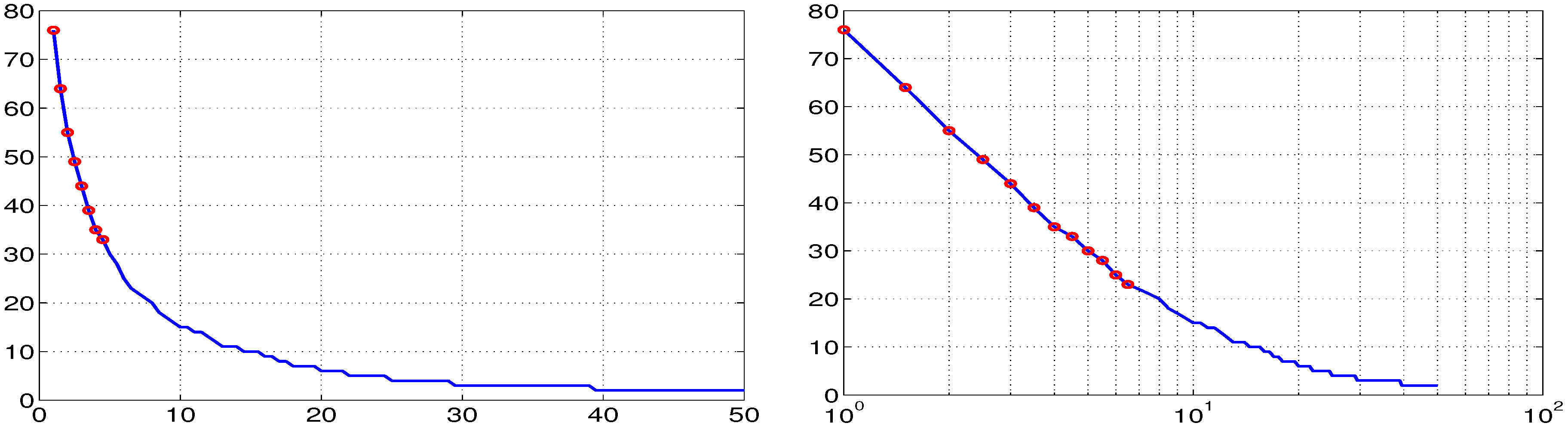
This procedure was then conducted for the 99 values $k=1,1.5,2,\cdots ,50$, and the optimal value of α, $\widehat{\alpha }\left(k\right)$, was determined. The results are shown in Figure 2. The left panel plots k versus $\widehat{\alpha }\left(k\right)$ and shows that the $\widehat{\alpha }$ behave as expected. The right panel shows the log plot, which reveals an almost linear structure of $\widehat{\alpha }$ for low values of k.

Figure 2. (Left) Plots $\widehat{\alpha }\left(k\right)$ versus k for $n=1000$, each obtained via simulation using 25,000 replications; (Right) The same, but using a log scale.

Figure 2. (Left) Plots $\widehat{\alpha }\left(k\right)$ versus k for $n=1000$, each obtained via simulation using 25,000 replications; (Right) The same, but using a log scale.

This can be used to construct a simple approximation to the relationship between k and $\widehat{\alpha }\left(k\right)$. The first five observations ($v=1,1.5,\cdots ,3$) are virtually perfectly modeled as:

$$\widehat{\alpha }\left(k\right)\approx \breve{\alpha }\left(k\right):=\mathrm{round}\left(75.8264-29.2699log\left(k\right)\right),1\le k\le 3$$

(5)

with an $R^2$ of 0.9993. For $3<k\le 33$, we obtain:

$$\widehat{\alpha }\left(k\right)\approx \breve{\alpha }\left(v\right):=\mathrm{round}\left(81.6637-40.5658logk+5.1540{\left(logk\right)}^2\right),3<k\le 33$$

(6)

with $R^2=0.9983$. For $33\le k<50$, we take $\breve{\alpha }\left(k\right)=3$. The same exercise was repeated for different sample sizes and, conveniently, the optimal values of α do not depend on the sample size, at least for n between 250 and 2000.

The procedure for estimating $a_0$ is then as follows. First take $a_0$ to be the sample median of the returns data, say ${\widehat{a}}_0^{\left(1\right)}=\text{median}\left(R_t\right)$, and apply the fixed APARCH filter discussed below to the location-adjusted returns $R_t-{\widehat{a}}_0^{\left(1\right)}$. This results in a set of data, say ${\mathbf{Z}}^{(1)}=\left(Z_1^{\left(1\right)},\cdots ,Z_T^{(1)}\right)$, which are (close to) i.i.d., with the unit scale term. Based on ${\mathbf{Z}}^{\left(1\right)}$, compute the estimators of k and $\gamma$, which could be done using MLE, or a lookup table, as discussed in Section 2.3. Next, based on $\widehat{k}$, use Equation (5) or Equation (6) to determine the optimal trimming value α, say ${\alpha }_{*}^{\left(1\right)}$. Finally, let ${\widehat{a}}_0^{\left(2\right)}=\text{trim}\left({\mathbf{Z}}^{\left(1\right)}+{\widehat{a}}_0^{\left(1\right)},{\alpha }_{*}^{\left(1\right)}\right)$. This can be repeated, applying the GARCH filter to $R_t-{\widehat{a}}_0^{\left(2\right)}$ to get ${\mathbf{Z}}^{\left(2\right)}$; then, obtain $\widehat{k}$ and $\widehat{\gamma }$ (from, say, a lookup table); use Equation (5) or Equation (6) to get ${\alpha }_{*}^{\left(2\right)}$, and set ${\widehat{a}}_0^{\left(3\right)}=\text{trim}\left({\mathbf{Z}}^{\left(2\right)}+{\widehat{a}}_0^{\left(2\right)},{\alpha }_{*}^{\left(2\right)}\right)$, etc.

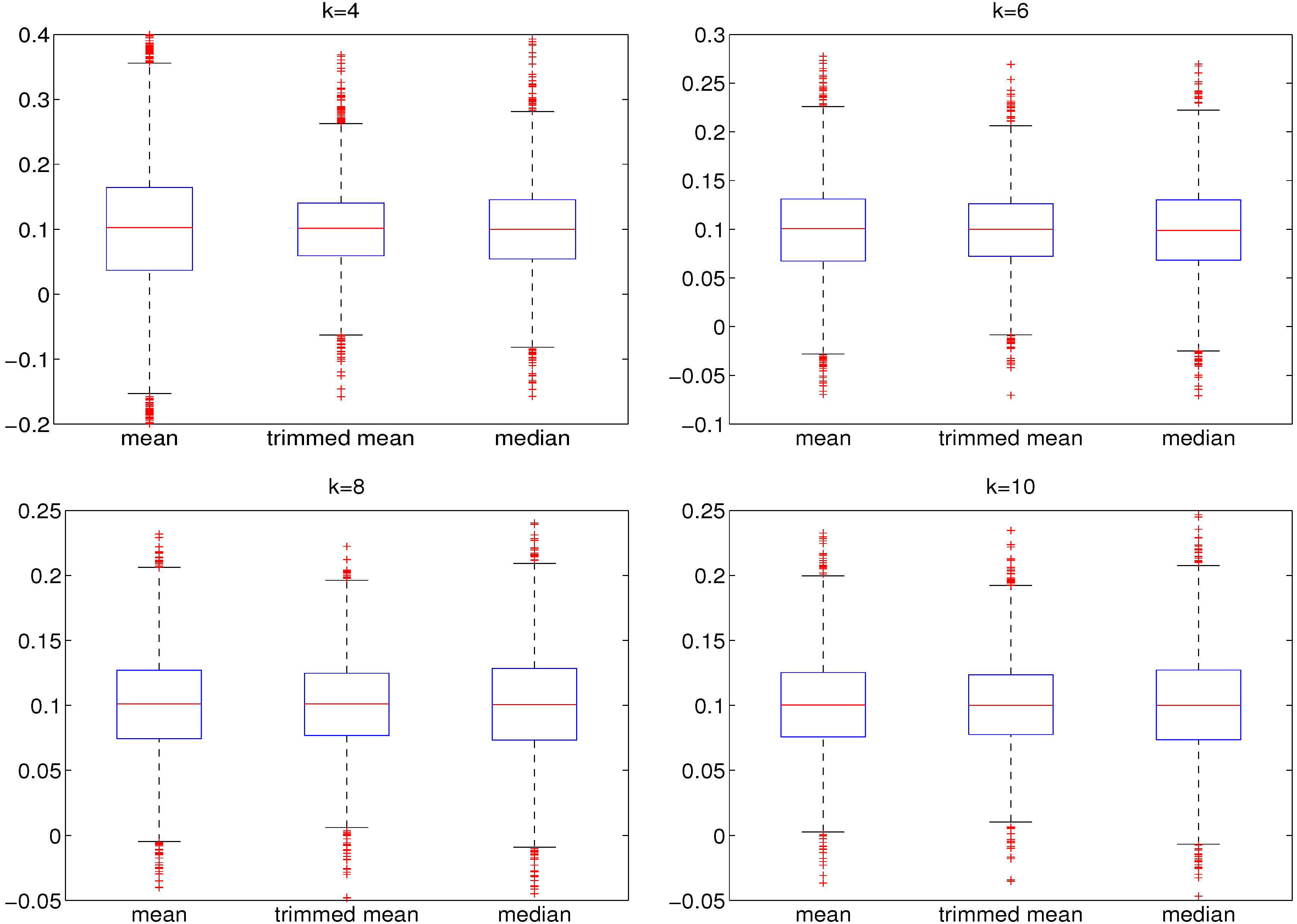
The devised method converged after three or four iterations in all simulation studies conducted. Figure 3 shows the comparison of the sample mean, the sample median and our iterated (three iterations used) sample trimmed mean estimator. The latter performs superior to the sample mean and sample median in all cases and yields a lower spread of estimates around the true value. The results shown in Figure 3 are qualitatively the same when the MLE is employed in lieu of using a lookup table; see Table 1. Qualitatively similar results were found to hold for a sample size of 250.

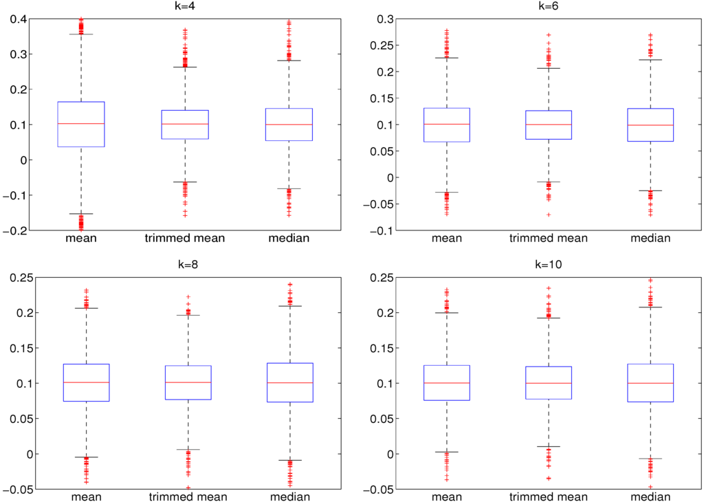
Figure 3. Boxplots of 5000 estimates of $a_0$ based on simulated data of length $T=1000$, generated from a t-GARCH model with parameters $a_0=0.1$, $c_0=0.04$, $c_1=0.05$, $d_1=0.09$, for different degrees of freedom $k=\text{4,6,8,10}$. For estimating the degrees of freedom, the lookup table-based estimation is used. Results for the MLE are qualitatively identical. The (iterative) trimmed mean procedure is stopped after three iterations.

Figure 3. Boxplots of 5000 estimates of $a_0$ based on simulated data of length $T=1000$, generated from a t-GARCH model with parameters $a_0=0.1$, $c_0=0.04$, $c_1=0.05$, $d_1=0.09$, for different degrees of freedom $k=\text{4,6,8,10}$. For estimating the degrees of freedom, the lookup table-based estimation is used. Results for the MLE are qualitatively identical. The (iterative) trimmed mean procedure is stopped after three iterations.

2.2.2. Use of Fixed GARCH Parameters

We first provide simulation-based evidence indicating the potential plausibility of the method to deliver similar density (and, thus, VaR and ES) predictions as full MLE estimation. One can view both models as special (extreme) cases of shrinkage-based MLE, with the optimal amount of shrinkage most likely not at either of these two extremes. We compare: (i) the variation of estimated NCT-GARCH parameters on typical financial returns data; with (ii) the variation of the MLE from simulation of the NCT-GARCH process using a typical parameter vector as the true values. If the variation in (i) is smaller than that in (ii), then it stands to reason that the estimation of the GARCH parameters can be forgone without great loss of accuracy and replaced by typical values obtained in (i) (for which we choose $c_0=0.04$, $c_1=0.05$ and $d_1=0.90$).

As a demonstration, we consider the daily percentage log returns of the 30 components of the DJIA from Wharton/CRSP(as used in April 2013), from 1 January 1993, until 31 December 2012. For (i), we use non-overlapping windows of a length of 1000 (yielding 150 sets of parameter estimates), and the results are shown in Figure 4. (Although we are only concerned with the GARCH parameters, we show all six parameters for completeness.)

Table 1. Root mean squared errors (RMSE) for the sample mean, the sample trimmed mean procedure from Section 2.2.1 and the sample median. Values are based on 5000 estimates of $a_0$ using simulated data generated from a t-GARCH model with parameters $a_0=0.1$, $c_0=0.04$, $c_1=0.05$, $d_1=0.90$, for different degrees of freedom $k=4,6,8,10$. The (iterative) trimmed mean procedure is stopped after three iterations. For estimating the degrees of freedom of the conditional Student’s t distribution, MLE and lookup table estimation (LTE) are used. GARCH parameters are fixed. Entries in boldface denote the smallest RMSE.

Model	Number Of Entries	Number of Quantiles	k	RMSE of the Mean	RMSE of the Trimmed Mean Procedure	RMSE of the Median
$T=250$
MLE			4	0.372	0.191	0.204
MLE			6	0.098	0.083	0.095
MLE			8	0.080	0.073	0.085
MLE			10	0.072	0.069	0.082
LTE	3621	6	4	0.308	0.183	0.197
LTE	3621	6	6	0.097	0.085	0.097
LTE	3621	6	8	0.080	0.073	0.085
LTE	3621	6	10	0.074	0.070	0.083
LTE	56,481	41	4	0.302	0.168	0.181
LTE	56,481	41	6	0.097	0.085	0.097
LTE	56,481	41	8	0.079	0.073	0.085
LTE	56,481	41	10	0.074	0.070	0.082
$T=1000$
MLE			4	0.171	0.064	0.071
MLE			6	0.049	0.041	0.047
MLE			8	0.040	0.037	0.042
MLE			10	0.036	0.033	0.040
LTE	3621	6	4	0.153	0.065	0.072
LTE	3621	6	6	0.048	0.040	0.047
LTE	3621	6	8	0.040	0.036	0.042
LTE	3621	6	10	0.036	0.034	0.040
LTE	56,481	41	4	0.272	0.064	0.070
LTE	56,481	41	6	0.049	0.041	0.047
LTE	56,481	41	8	0.040	0.036	0.042
LTE	56,481	41	10	0.037	0.034	0.040

Table 1. Root mean squared errors (RMSE) for the sample mean, the sample trimmed mean procedure from Section 2.2.1 and the sample median. Values are based on 5000 estimates of $a_0$ using simulated data generated from a t-GARCH model with parameters $a_0=0.1$, $c_0=0.04$, $c_1=0.05$, $d_1=0.90$, for different degrees of freedom $k=4,6,8,10$. The (iterative) trimmed mean procedure is stopped after three iterations. For estimating the degrees of freedom of the conditional Student’s t distribution, MLE and lookup table estimation (LTE) are used. GARCH parameters are fixed. Entries in boldface denote the smallest RMSE.

Model	Number Of Entries	Number of Quantiles	k	RMSE of the Mean	RMSE of the Trimmed Mean Procedure	RMSE of the Median
$T=250$
MLE			4	0.372	0.191	0.204
MLE			6	0.098	0.083	0.095
MLE			8	0.080	0.073	0.085
MLE			10	0.072	0.069	0.082
LTE	3621	6	4	0.308	0.183	0.197
LTE	3621	6	6	0.097	0.085	0.097
LTE	3621	6	8	0.080	0.073	0.085
LTE	3621	6	10	0.074	0.070	0.083
LTE	56,481	41	4	0.302	0.168	0.181
LTE	56,481	41	6	0.097	0.085	0.097
LTE	56,481	41	8	0.079	0.073	0.085
LTE	56,481	41	10	0.074	0.070	0.082
$T=1000$
MLE			4	0.171	0.064	0.071
MLE			6	0.049	0.041	0.047
MLE			8	0.040	0.037	0.042
MLE			10	0.036	0.033	0.040
LTE	3621	6	4	0.153	0.065	0.072
LTE	3621	6	6	0.048	0.040	0.047
LTE	3621	6	8	0.040	0.036	0.042
LTE	3621	6	10	0.036	0.034	0.040
LTE	56,481	41	4	0.272	0.064	0.070
LTE	56,481	41	6	0.049	0.041	0.047
LTE	56,481	41	8	0.040	0.036	0.042
LTE	56,481	41	10	0.037	0.034	0.040

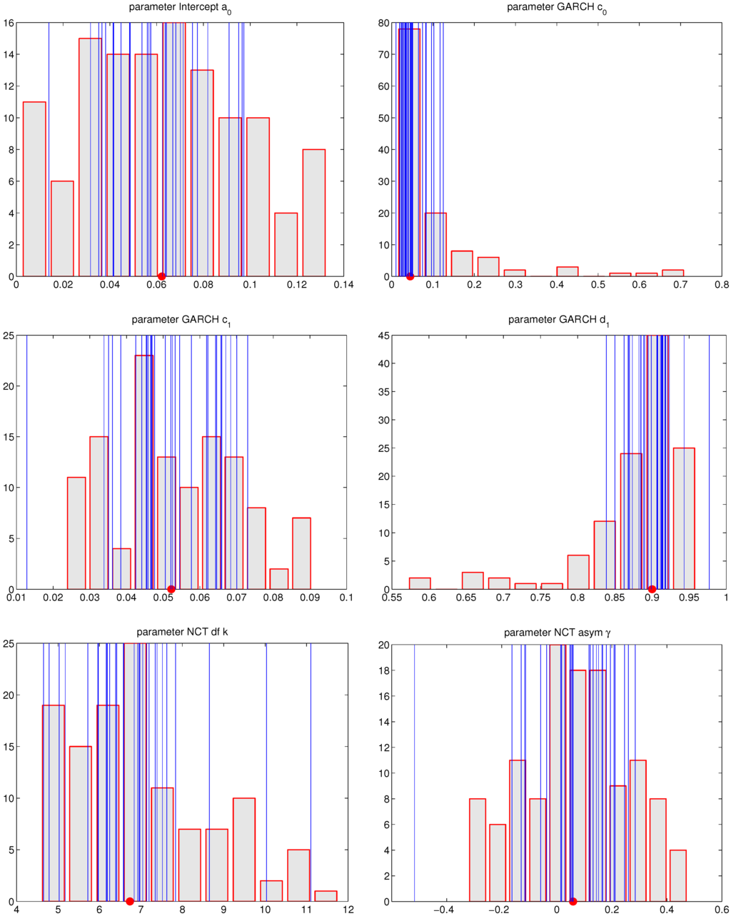
Figure 4. MLE parameter estimates corresponding to the NCT-GARCH model, for the DJIA-30 data, using non-overlapping windows of length $T=1000$, over 20 years of data and the 30 time series. The circle on the x-axis indicates the median of the data. Blue lines refer to the average parameter value for each of the 30 assets.

Figure 4. MLE parameter estimates corresponding to the NCT-GARCH model, for the DJIA-30 data, using non-overlapping windows of length $T=1000$, over 20 years of data and the 30 time series. The circle on the x-axis indicates the median of the data. Blue lines refer to the average parameter value for each of the 30 assets.

This can be compared to Figure 5, which shows the computation corresponding to (ii), i.e., the MLE simulation results based on series of length $T=1000$, generated from an NCT-GARCH process with parameters $a_0=0.06$, $c_0=0.05$, $c_1=0.05$, $d_1=0.90$, $k=7$, and $\gamma =0.05$. The corresponding two figures for $T=250$ were also computed and are similar, though look even less Gaussian than the case with $T=1000$; and are available upon request. Also, the simulation in (ii) was conducted using $T=25,000$, to confirm the consistency and asymptotic normality of the estimators. We see that the variation of (i) is, as hoped, smaller than that of (ii), for GARCH parameters $c_0$ and $c_1$, though it is not quite the case for parameter $d_1$, because of the elongated left tail in the distribution for $d_1$ in Figure 4. However, most of the mass is indeed centered around the value $0.90$. As such, this exercise lends some evidence that we can forgo the estimation of the GARCH parameters, but it remains to be seen what effect this has on out-of-sample performance for density and VaR prediction. This is done below in Section 3.

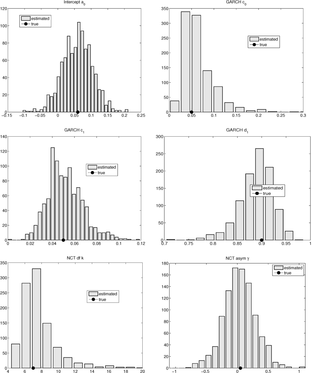
Figure 5. MLE Parameter estimates corresponding to the NCT-GARCH model, for simulated noncentral t (NCT) GARCH data, using length $T=1000$ and 1000 replications. The circle on the x-axis indicates the median of the data.

Figure 5. MLE Parameter estimates corresponding to the NCT-GARCH model, for simulated noncentral t (NCT) GARCH data, using length $T=1000$ and 1000 replications. The circle on the x-axis indicates the median of the data.

2.2.3. Fixed GARCH Parameters and APARCH

The previous exercise was initially conducted using the APARCH model, based on 250 observations, this being one of the two sample sizes we chose to use in our forecast demonstration below. The reason for this sample size of approximately one year of daily trading data is to help avoid the effects of model misspecification, such as regime switching; see, e.g., Chavez-Demoulin et al. [17], or, more generally, to account for the fact that the proposed model is surely not the true data generating process through all of time; see the discussion and evidence in Paolella [18].

Using a sample size of 250 and estimating via MLE all of the parameters of the NCT-APARCH model, it is found that the estimated asymmetry (leverage effect) parameter is rather erratic, when viewed over moving windows through time, and often approaches (and touches) its upper boundary value of one. To rule out any computational errors, simulations were conducted. When using a sample size of 250, it was found that the final ML estimates are very sensitive to the choice of starting values and appear to result in biased estimation of the asymmetry parameter. However, when using very large sample sizes (e.g., 25,000), the maximum likelihood estimator looks as one would expect, namely virtually perfectly Gaussian and centered around the true parameter values, this having been achieved using any reasonable set of starting values, not just the true ones.

Given the problematic asymmetry parameter in small sample sizes, we first select the three parameters associated with the traditional GARCH model (with NCT innovations) and, then, conditional on those, choose the optimal asymmetry parameter in the APARCH construction. In particular, we investigate the effect of allowing for a non-zero asymmetry parameter ${\gamma }_1$ in Equation (2) with respect to out-of-sample prediction quality. To determine the optimal choice of ${\gamma }_1$, we perform different out-of-sample forecast studies, each with a fixed ${\gamma }_1$ coefficient. (To speed up estimation, we employ the table lookup method for the NCT parameters, as described in the next section.)

Figure 6 shows the results of VaR performance and prediction quality, the latter measured by evaluating the log predicted NCT density at the realized returns, as done in Paolella [18] and Paolella and Polak [19]. This was conducted for two sample sizes, 250 and 1000, and the results are remarkably similar. Clearly, the NCT-APARCH model (with fixed GARCH parameters) has superior performance for most choices of ${\gamma }_1$, with the number of VaR violations being closer to its expected value. A similar result is observed, but less pronounced, in terms of prediction quality: for $0.25\le {\gamma }_1\le 0.55$, the NCT-APARCH model outperforms the GARCH case. From these plots, it appears that taking ${\gamma }_1=0.4$ is the optimal choice to improve the forecast quality. We subsequently use this in all of the following empirical examples.

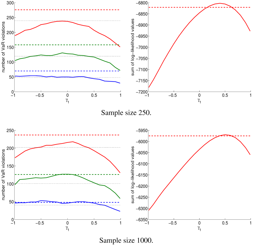
Figure 6. An illustration of the effect of varying the APARCH parameter on the number of VaR violations (left) and the sum of log-likelihood values (right) evaluated at the realized return given the predicted density of the portfolio return. Results are out-of-sample for the period 4 January 1993 to 31 December 2012, obtained from rolling window exercises with windows of a length of 250 (4787 forecasts) and 1000 (4037 forecasts), respectively. The data set under study is the 20-year sequence of daily returns (percentage log-returns) of the equally weighted portfolio of DJIA30components (as of April 2013). Dashed lines refer to the NCT-GARCH model, solid lines to the NCT-APARCH model with ${\gamma }_1$ being varied. In the case of NCT-GARCH, model parameters are estimated by MLE, while for NCT-APARCH, $a_0$ is obtained using the trimmed mean procedure in Section 2.2.1, and the GARCH parameters are fixed according to Section 2.2.2, i.e., we use $c_0=0.04$, $c_1=0.05$, $d_1=0.90$. Dotted lines in the left panel depict the expected number of VaR violations at the 1% (lower lines; blue), 2.5% (middle lines; green) and 5% (upper lines; red) significance level, respectively.

Figure 6. An illustration of the effect of varying the APARCH parameter on the number of VaR violations (left) and the sum of log-likelihood values (right) evaluated at the realized return given the predicted density of the portfolio return. Results are out-of-sample for the period 4 January 1993 to 31 December 2012, obtained from rolling window exercises with windows of a length of 250 (4787 forecasts) and 1000 (4037 forecasts), respectively. The data set under study is the 20-year sequence of daily returns (percentage log-returns) of the equally weighted portfolio of DJIA30components (as of April 2013). Dashed lines refer to the NCT-GARCH model, solid lines to the NCT-APARCH model with ${\gamma }_1$ being varied. In the case of NCT-GARCH, model parameters are estimated by MLE, while for NCT-APARCH, $a_0$ is obtained using the trimmed mean procedure in Section 2.2.1, and the GARCH parameters are fixed according to Section 2.2.2, i.e., we use $c_0=0.04$, $c_1=0.05$, $d_1=0.90$. Dotted lines in the left panel depict the expected number of VaR violations at the 1% (lower lines; blue), 2.5% (middle lines; green) and 5% (upper lines; red) significance level, respectively.

2.3. Lookup Table

To further speed up the calculation of the NCT-APARCH model, we propose the use of a lookup table. In particular, we replace the ML estimation of the two shape parameters by values obtained from a pre-computed table, using a function of the sample quantiles. Based on a tight grid of values for parameters k and $\gamma$, for every pair of $\{k,\gamma \}$, the set of corresponding quantiles $\{Q_1,\cdots ,Q_m\}$ is computed (with each $Q_i$ obtained by numerically inverting the NCT cdf). For example, with $m=21$, we choose quantiles corresponding to probabilities $\{0.01,0.05,0.10,0.15,\cdots ,0.95,0.99\}$. With the completed table, parameter estimation is conducted by finding in the table that pair $\{k,\gamma \}$ for which:

$$\sum _{i=1}^m{w}_i{\left({\widehat{Q}}_i-Q_i\right)}^2$$

(7)

is minimized, where ${\widehat{Q}}_i$ refers to the sample counterpart of $Q_i$ and ${(w_1,\cdots ,w_m)}^{\prime }$ is the vector of weights obtained using the asymptotic distribution, i.e., $w_j=\sqrt{n}/{\sigma }_j$, $j=1,\cdots ,m$, where ${\sigma }_j=\sqrt{p_j(1-p_j)}/f\left(Q_j\right)$ with f being the NCT pdf and $p_j$ being the probability corresponding to quantile $Q_j$.

There are several tuning parameters to be chosen: the number m of quantiles, which quantiles, the size (granularity) of the lookup table and whether to use weighting or not, as it might not yield relatively high improvements in accuracy compared to its additional computational time.

For demonstrating the method, we consider four sets of quantiles $m=6,11,21,41$ and three table sizes $n=$ 3621, 14,241, 56,481. Table 2 shows the results of the simulation for a sample size of 250 and based on 1000 replications. Additional results for a sample size of 1000 are included in the working paper version of this document. As expected, both accuracy and computational time of the lookup table estimation (LTE) increase monotonically with m and the table size. Furthermore, it can be seen that the accuracy of the weighted lookup table estimator (wLTE) is better than the one of the non-weighted variant, but differences are minor. The wLTE, however, requires twice as much memory (for storing the weighting coefficients ${\omega }_i$) and, also, roughly, twice as many floating point operations. Hence, the non-weighted LTE is generally faster and, therefore, might be favorable in certain contexts. Furthermore, large tables are unlikely to fit into the processor’s (L2- or L3-) cache, which results in significantly slower computations times compared to the use of small tables that fit into cache memory. Compared to the MLE, a lookup table gives considerably lower computation times, in particular when the sample size is large.

The last line in Table 2, showing the MLE performance, is noteworthy. We see that the MLE is outperformed in terms of MSE by the most sophisticated lookup table method. This is important, as it demonstrates that even for a (traditionally, in statistics, large) sample size of 250, the MLE can be outperformed by alternative, simpler and faster estimation methods. In the working paper version of this document, a similar table is provided based on a sample size of 1000. It demonstrates that, asymptotically, the MLE will outperform all non-trivial (i.e., non-measure-zero) estimators, though the table lookup methods are still competitive.

Moreover, the table lookup approach is not limited to parameter estimates. It is straightforward to also return, e.g., exact VaR and ES values, as mentioned in Section 2.1. These can then be used to obtain the VaR and ES values corresponding to the NCT-APARCH density prediction, recalling that VaR and ES preserve location-scale transformations. This is the method we employ.

Table 2. Evaluation of estimation quality based on 1000 estimates of the (location-adjusted) NCT pdf in Equation (3) using simulated data (250 observations). The true parameters of the data generating process are $\mathit{\theta }={(k,\gamma )}^{\prime }={(7,0.05)}^{\prime }$. ML estimations are performed by MATLAB’s fminunc using $\mathit{\theta }={(10,0.2)}^{\prime }$ as the starting value and based on the approximate NCT density. In addition, parameter restrictions similar to those used for the lookup tables are imposed in ML estimations. Lookup tables are constructed based on an equally-spaced grid with step sizes given by $h_1$ and $h_2$, respectively.

Model	Number of Entries	Number of Quantiles	NCT dfk Steps in $[2,30]$	NCT asym. $\gamma$ Steps in $[-1,1]$	Average Runtime	Average Log-lik.	Average RMSE
LTE	3621	6	71	51	0.001 s	−391.9075	3.804
LTE	3621	11	71	51	0.001 s	−391.8002	3.732
LTE	3621	21	71	51	0.002 s	−391.5919	3.665
LTE	3621	41	71	51	0.004 s	−391.3617	3.585
			$h_1=0.4$	$h_2=0.04$
LTE	14,241	6	141	101	0.002 s	−391.9038	3.807
LTE	14,241	11	141	101	0.004 s	−391.7969	3.730
LTE	14,241	21	141	101	0.007 s	−391.5920	3.668
LTE	14,241	41	141	101	0.010 s	−391.3608	3.589
			$h_1=0.2$	$h_2=0.02$
LTE	56,481	6	281	201	0.008 s	−391.9032	3.807
LTE	56,481	11	281	201	0.010 s	−391.7977	3.730
LTE	56,481	21	281	201	0.030 s	−391.5900	3.669
LTE	56,481	41	281	201	0.050 s	−391.3601	3.589
			$h_1=0.1$	$h_2=0.01$
wLTE	3621	6	71	51	0.001 s	−391.6156	3.753
wLTE	3621	11	71	51	0.001 s	−391.4190	3.539
wLTE	3621	21	71	51	0.002 s	−391.3269	3.312
wLTE	3621	41	71	51	0.005 s	−391.3711	3.247
			$h_1=0.4$	$h_2=0.04$
wLTE	14,241	6	141	101	0.002 s	−391.6110	3.751
wLTE	14,241	11	141	101	0.005 s	−391.4177	3.541
wLTE	14,241	21	141	101	0.009 s	−391.3232	3.311
wLTE	14,241	41	141	101	0.020 s	−391.3687	3.242
			$h_1=0.2$	$h_2=0.02$
wLTE	56,481	6	281	201	0.010 s	−391.6123	3.752
wLTE	56,481	11	281	201	0.020 s	−391.4176	3.541
wLTE	56,481	21	281	201	0.040 s	−391.3234	3.312
wLTE	56,481	41	281	201	0.070 s	−391.3669	3.242
			$h_1=0.1$	$h_2=0.01$
MLE	–	–	–	–	0.068 s	−391.0015	3.470

Table 2. Evaluation of estimation quality based on 1000 estimates of the (location-adjusted) NCT pdf in Equation (3) using simulated data (250 observations). The true parameters of the data generating process are $\mathit{\theta }={(k,\gamma )}^{\prime }={(7,0.05)}^{\prime }$. ML estimations are performed by MATLAB’s fminunc using $\mathit{\theta }={(10,0.2)}^{\prime }$ as the starting value and based on the approximate NCT density. In addition, parameter restrictions similar to those used for the lookup tables are imposed in ML estimations. Lookup tables are constructed based on an equally-spaced grid with step sizes given by $h_1$ and $h_2$, respectively.

Model	Number of Entries	Number of Quantiles	NCT dfk Steps in $[2,30]$	NCT asym. $\gamma$ Steps in $[-1,1]$	Average Runtime	Average Log-lik.	Average RMSE
LTE	3621	6	71	51	0.001 s	−391.9075	3.804
LTE	3621	11	71	51	0.001 s	−391.8002	3.732
LTE	3621	21	71	51	0.002 s	−391.5919	3.665
LTE	3621	41	71	51	0.004 s	−391.3617	3.585
			$h_1=0.4$	$h_2=0.04$
LTE	14,241	6	141	101	0.002 s	−391.9038	3.807
LTE	14,241	11	141	101	0.004 s	−391.7969	3.730
LTE	14,241	21	141	101	0.007 s	−391.5920	3.668
LTE	14,241	41	141	101	0.010 s	−391.3608	3.589
			$h_1=0.2$	$h_2=0.02$
LTE	56,481	6	281	201	0.008 s	−391.9032	3.807
LTE	56,481	11	281	201	0.010 s	−391.7977	3.730
LTE	56,481	21	281	201	0.030 s	−391.5900	3.669
LTE	56,481	41	281	201	0.050 s	−391.3601	3.589
			$h_1=0.1$	$h_2=0.01$
wLTE	3621	6	71	51	0.001 s	−391.6156	3.753
wLTE	3621	11	71	51	0.001 s	−391.4190	3.539
wLTE	3621	21	71	51	0.002 s	−391.3269	3.312
wLTE	3621	41	71	51	0.005 s	−391.3711	3.247
			$h_1=0.4$	$h_2=0.04$
wLTE	14,241	6	141	101	0.002 s	−391.6110	3.751
wLTE	14,241	11	141	101	0.005 s	−391.4177	3.541
wLTE	14,241	21	141	101	0.009 s	−391.3232	3.311
wLTE	14,241	41	141	101	0.020 s	−391.3687	3.242
			$h_1=0.2$	$h_2=0.02$
wLTE	56,481	6	281	201	0.010 s	−391.6123	3.752
wLTE	56,481	11	281	201	0.020 s	−391.4176	3.541
wLTE	56,481	21	281	201	0.040 s	−391.3234	3.312
wLTE	56,481	41	281	201	0.070 s	−391.3669	3.242
			$h_1=0.1$	$h_2=0.01$
MLE	–	–	–	–	0.068 s	−391.0015	3.470

3. Density and VaR Forecasting

To evaluate the performance of the NCT-APARCH model estimated using the trimmed mean procedure for $a_0$, fixed APARCH parameters and the lookup table, we perform some standard tests on the out-of-sample VaR and also examine the ranking of out-of-sample predictive log likelihood statistics, all using real data. In addition, we compare the models’s performance to that of two competing models that have been shown to perform extraordinarily well and, thus, serve as reference standards. These are the mixed-normal-GARCH ([20,21]), and its extension, the mixed-normal-GARCH model with time-varying mixing weights ([3]). They address volatility clustering, fat-tails, asymmetry and, also, give rise to rich volatility dynamics not possible with traditional (single-component) GARCH models. Extensive out-of-sample forecast exercises in Kuester et al. [2] and Haas et al. [3] have confirmed that these models deliver highly accurate VaR forecasts. The models are briefly summarized in Appendix B.

Analogously to Section 2.2.3, where the choice of the APARCH parameter ${\gamma }_1$ is investigated, we focus on density and VaR forecasting quality among the various competing models. For VaR quality, the number of realized VaR violations is considered, while the density forecast quality is measured by the sum of log-likelihood values of the predictive density, evaluated at the realized return. As before, we use the sequence of daily (percentage log-) returns of DJIA30 components (i.e., the DJIA constituents as of April 2013). The comparison spans the period 4 January 1993 to 31 December 2012, and comprises: (i) the 4787 one-step-ahead forecasts obtained from a rolling window with size 250; and similarly; (ii) the 4037 forecasts for a window size of 1000.

The models under study are:

• the MixN-GARCH($3,2$) and the TW-MixN-GARCH($2,2$) models (see Appendix B), estimated via the extended augmented likelihood estimator (EALE), as introduced in Broda et al. [22]; also see Haas et al. [3],
• the NCT-GARCH model, given by Equation (2) with ${\gamma }_1=0$, estimated by MLE using the NCT density approximation detailed in Appendix A, and
• the NCT-APARCH model, given by Equation (2) with $a_0$ computed, as described in Section 2.2.1, and fixed parameter values, as described in Section 2.2.2 and Section 2.2.3.

The first example uses the equally weighted portfolio of these 30 stocks, which is a common choice in many risk testing applications; see, e.g., Santos et al. [23]. The ability of the “$1/N$ portfolio” to outperform even sophisticated allocation methods goes back at least to Bloomfield et al. [24] and is further detailed in DeMiguel et al. [25] and Brown et al. [26] and the references therein. Table 3 and Table 4 summarize the out-of-sample results for moving window sizes of 250 and 1000, respectively. We report realized violation frequencies for the predictive VaR at the 1%, 2.5% and 5% significance level and test statistics for unconditional coverage (LLUC), independence (LLIND) and conditional coverage (LLCC), according to the tests proposed in Christoffersen [27]. The following relationship holds, ${\text{LR}}_{\text{CC}}={\text{LR}}_{\text{UC}}+{\text{LR}}_{\text{IND}}$, where asymptotically ${\text{LR}}_{\text{UC}}\sim {\chi }^2\left(1\right)$ independent of ${\text{LR}}_{\text{IND}}\sim {\chi }^2\left(1\right)$, and thus, ${\text{LR}}_{\text{CC}}\sim {\chi }^2\left(2\right)$.

Table 3. Out-of-sample forecast results based on the daily returns for the equally weighted portfolio. The first section of the table shows the empirical violation frequency for various models and three probability levels, for the univariate time series corresponding to the equally weighted portfolio of the 30 DJIAstocks, from January 1 1993 to December 31 2012, using rolling windows of a size of 250 and a step size of one day, resulting in 4787 predicted observations. Values reported for unconditional coverage (LLUC), independence (LLIND) and conditional coverage (LLCC) are the test statistics, as described in Christoffersen [27]. Entries in boldface denote the best outcomes. ***, **, and * denote significance at the 1%, 5% and 10% levels, respectively. SPLL is short for sum of (realized) predicted log-likelihood values. The following lookup tables are used, (a): Six quantiles, 3621 entries, first table in Table 2; (b): 41 quantiles, 3621 entries, fourth table in Table 2; and (c): 41 quantiles, 56,481 entries, twelfth table in Table 2. EALE, extended augmented likelihood estimator.

Model	Estimation	$a_0$		1% VaR	2.5% VaR	5% VaR
Empirical violation frequency							and SPLL
MixN-GARCH($3,2$)	EALE	jointly		1.36	3.11	5.70	−6864.52
TW-MixN-GARCH($2,2$)	EALE	jointly		1.32	3.05	5.62	−6879.26
NCT-APARCH (a)	LTE	tr. mean		1.07	2.38	4.49	−6802.75
NCT-APARCH (b)	LTE	tr. mean		0.94	2.53	4.49	−6796.98
NCT-APARCH (c)	LTE	tr. mean		0.94	2.53	4.49	−6797.06
NCT-GARCH	MLE	jointly		1.69	3.51	6.23	−6995.05
NCT-APARCH	MLE	jointly		1.59	3.36	5.93	−6918.63
NCT-APARCH (b)	LTE	median		0.919	2.444	4.324	−6806.1
NCT-APARCH (b)	wLTE	tr. mean		0.919	2.507	4.303	−6799.4
LLCC
MixN-GARCH($3,2$)	EALE	jointly		7.37 **	7.98 **	6.10 **
TW-MixN-GARCH($2,2$)	EALE	jointly		4.43	6.09 **	3.99
NCT-APARCH (a)	LTE	tr. mean		0.52	0.49	2.88
NCT-APARCH (b)	LTE	tr. mean		0.76	0.45	2.70
NCT-APARCH (c)	LTE	tr. mean		0.76	0.45	2.70
NCT-GARCH	MLE	jointly		19.45 ***	21.68 ***	15.79 ***
NCT-APARCH	MLE	jointly		14.63 ***	13.31 ***	8.40 **
LLUC
MixN-GARCH($3,2$)	EALE	jointly		5.58 **	6.86 ***	4.79 **
TW-MixN-GARCH($2,2$)	EALE	jointly		4.40 **	5.57 **	3.74 *
NCT-APARCH (a)	LTE	tr. mean		0.20	0.28	2.69
NCT-APARCH (b)	LTE	tr. mean		0.18	0.02	2.69
NCT-APARCH (c)	LTE	tr. mean		0.18	0.02	2.69
NCT-GARCH	MLE	jointly		19.19 ***	17.84 ***	14.11 ***
NCT-APARCH	MLE	jointly		14.18 ***	13.25 ***	8.31 ***
LLIND
MixN-GARCH($3,2$)	EALE	jointly		1.79	1.12	1.31
TW-MixN-GARCH($2,2$)	EALE	jointly		0.03	0.52	0.25
NCT-APARCH (a)	LTE	tr. mean		0.31	0.22	0.20
NCT-APARCH (b)	LTE	tr. mean		0.58	0.44	0.01
NCT-APARCH (c)	LTE	tr. mean		0.58	0.44	0.01
NCT-GARCH	MLE	jointly		0.26	3.84 *	1.68
NCT-APARCH	MLE	jointly		0.45	0.07	0.09

Table 3. Out-of-sample forecast results based on the daily returns for the equally weighted portfolio. The first section of the table shows the empirical violation frequency for various models and three probability levels, for the univariate time series corresponding to the equally weighted portfolio of the 30 DJIAstocks, from January 1 1993 to December 31 2012, using rolling windows of a size of 250 and a step size of one day, resulting in 4787 predicted observations. Values reported for unconditional coverage (LLUC), independence (LLIND) and conditional coverage (LLCC) are the test statistics, as described in Christoffersen [27]. Entries in boldface denote the best outcomes. ***, **, and * denote significance at the 1%, 5% and 10% levels, respectively. SPLL is short for sum of (realized) predicted log-likelihood values. The following lookup tables are used, (a): Six quantiles, 3621 entries, first table in Table 2; (b): 41 quantiles, 3621 entries, fourth table in Table 2; and (c): 41 quantiles, 56,481 entries, twelfth table in Table 2. EALE, extended augmented likelihood estimator.

Model	Estimation	$a_0$		1% VaR	2.5% VaR	5% VaR
Empirical violation frequency							and SPLL
MixN-GARCH($3,2$)	EALE	jointly		1.36	3.11	5.70	−6864.52
TW-MixN-GARCH($2,2$)	EALE	jointly		1.32	3.05	5.62	−6879.26
NCT-APARCH (a)	LTE	tr. mean		1.07	2.38	4.49	−6802.75
NCT-APARCH (b)	LTE	tr. mean		0.94	2.53	4.49	−6796.98
NCT-APARCH (c)	LTE	tr. mean		0.94	2.53	4.49	−6797.06
NCT-GARCH	MLE	jointly		1.69	3.51	6.23	−6995.05
NCT-APARCH	MLE	jointly		1.59	3.36	5.93	−6918.63
NCT-APARCH (b)	LTE	median		0.919	2.444	4.324	−6806.1
NCT-APARCH (b)	wLTE	tr. mean		0.919	2.507	4.303	−6799.4
LLCC
MixN-GARCH($3,2$)	EALE	jointly		7.37 **	7.98 **	6.10 **
TW-MixN-GARCH($2,2$)	EALE	jointly		4.43	6.09 **	3.99
NCT-APARCH (a)	LTE	tr. mean		0.52	0.49	2.88
NCT-APARCH (b)	LTE	tr. mean		0.76	0.45	2.70
NCT-APARCH (c)	LTE	tr. mean		0.76	0.45	2.70
NCT-GARCH	MLE	jointly		19.45 ***	21.68 ***	15.79 ***
NCT-APARCH	MLE	jointly		14.63 ***	13.31 ***	8.40 **
LLUC
MixN-GARCH($3,2$)	EALE	jointly		5.58 **	6.86 ***	4.79 **
TW-MixN-GARCH($2,2$)	EALE	jointly		4.40 **	5.57 **	3.74 *
NCT-APARCH (a)	LTE	tr. mean		0.20	0.28	2.69
NCT-APARCH (b)	LTE	tr. mean		0.18	0.02	2.69
NCT-APARCH (c)	LTE	tr. mean		0.18	0.02	2.69
NCT-GARCH	MLE	jointly		19.19 ***	17.84 ***	14.11 ***
NCT-APARCH	MLE	jointly		14.18 ***	13.25 ***	8.31 ***
LLIND
MixN-GARCH($3,2$)	EALE	jointly		1.79	1.12	1.31
TW-MixN-GARCH($2,2$)	EALE	jointly		0.03	0.52	0.25
NCT-APARCH (a)	LTE	tr. mean		0.31	0.22	0.20
NCT-APARCH (b)	LTE	tr. mean		0.58	0.44	0.01
NCT-APARCH (c)	LTE	tr. mean		0.58	0.44	0.01
NCT-GARCH	MLE	jointly		0.26	3.84 *	1.68
NCT-APARCH	MLE	jointly		0.45	0.07	0.09

Table 4. Similar to Table 3, but based on rolling windows of a size of 1000 days (4037 forecasts).

Model	Estimation	$a_0$		1% VaR	2.5% VaR	5% VaR
empirical violation frequency							and SPLL
MixN-GARCH($3,2$)	EALE	jointly		1.11	2.95	5.42	−5996.51
TW-MixN-GARCH($2,2$)	EALE	jointly		1.21	2.77	5.38	−5993.15
NCT-APARCH (a)	LTE	tr. mean		0.99	2.58	4.90	−5969.88
NCT-APARCH (b)	LTE	tr. mean		1.19	2.65	4.90	−5970.83
NCT-APARCH (c)	LTE	tr. mean		1.16	2.65	4.90	−5970.88
NCT-GARCH	MLE	jointly		1.19	3.12	5.87	−5974.90
NCT-APARCH	MLE	jointly		1.16	2.97	5.52	−5905.26
NCT-APARCH (b)	LTE	median		1.19	2.70	4.98	−5973.99
NCT-APARCH (b)	wLTE	tr. mean		1.29	2.75	4.95	−5971.10
LLCC
MixN-GARCH($3,2$)	EALE	jointly		1.53	3.96	1.50
TW-MixN-GARCH($2,2$)	EALE	jointly		2.95	1.21	1.19
NCT-APARCH (a)	LTE	tr. mean		0.80	0.30	0.09
NCT-APARCH (b)	LTE	tr. mean		2.53	0.66	0.14
NCT-APARCH (c)	LTE	tr. mean		2.16	0.66	0.14
NCT-GARCH	MLE	jointly		2.53	5.94 *	6.47 **
NCT-APARCH	MLE	jointly		2.16	4.36	2.79
LLUC
MixN-GARCH($3,2$)	EALE	jointly		0.52	3.15 *	1.50
TW-MixN-GARCH($2,2$)	EALE	jointly		1.75	1.21	1.18
NCT-APARCH (a)	LTE	tr. mean		3.3e-3	0.10	0.08
NCT-APARCH (b)	LTE	tr. mean		1.38	0.37	0.08
NCT-APARCH (c)	LTE	tr. mean		1.05	0.37	0.08
NCT-GARCH	MLE	jointly		1.38	5.94 **	6.14 **
NCT-APARCH	MLE	jointly		1.05	3.50 *	2.27
LLIND
MixN-GARCH($3,2$)	EALE	jointly		1.01	0.81	1.3e-3
TW-MixN-GARCH($2,2$)	EALE	jointly		1.20	4.0e-3	0.01
NCT-APARCH (a)	LTE	tr. mean		0.80	0.20	0.01
NCT-APARCH (b)	LTE	tr. mean		1.16	0.29	0.06
NCT-APARCH (c)	LTE	tr. mean		1.11	0.29	0.06
NCT-GARCH	MLE	jointly		1.16	1.2e-3	0.34
NCT-APARCH	MLE	jointly		1.11	0.86	0.52

Table 4. Similar to Table 3, but based on rolling windows of a size of 1000 days (4037 forecasts).

Model	Estimation	$a_0$		1% VaR	2.5% VaR	5% VaR
empirical violation frequency							and SPLL
MixN-GARCH($3,2$)	EALE	jointly		1.11	2.95	5.42	−5996.51
TW-MixN-GARCH($2,2$)	EALE	jointly		1.21	2.77	5.38	−5993.15
NCT-APARCH (a)	LTE	tr. mean		0.99	2.58	4.90	−5969.88
NCT-APARCH (b)	LTE	tr. mean		1.19	2.65	4.90	−5970.83
NCT-APARCH (c)	LTE	tr. mean		1.16	2.65	4.90	−5970.88
NCT-GARCH	MLE	jointly		1.19	3.12	5.87	−5974.90
NCT-APARCH	MLE	jointly		1.16	2.97	5.52	−5905.26
NCT-APARCH (b)	LTE	median		1.19	2.70	4.98	−5973.99
NCT-APARCH (b)	wLTE	tr. mean		1.29	2.75	4.95	−5971.10
LLCC
MixN-GARCH($3,2$)	EALE	jointly		1.53	3.96	1.50
TW-MixN-GARCH($2,2$)	EALE	jointly		2.95	1.21	1.19
NCT-APARCH (a)	LTE	tr. mean		0.80	0.30	0.09
NCT-APARCH (b)	LTE	tr. mean		2.53	0.66	0.14
NCT-APARCH (c)	LTE	tr. mean		2.16	0.66	0.14
NCT-GARCH	MLE	jointly		2.53	5.94 *	6.47 **
NCT-APARCH	MLE	jointly		2.16	4.36	2.79
LLUC
MixN-GARCH($3,2$)	EALE	jointly		0.52	3.15 *	1.50
TW-MixN-GARCH($2,2$)	EALE	jointly		1.75	1.21	1.18
NCT-APARCH (a)	LTE	tr. mean		3.3e-3	0.10	0.08
NCT-APARCH (b)	LTE	tr. mean		1.38	0.37	0.08
NCT-APARCH (c)	LTE	tr. mean		1.05	0.37	0.08
NCT-GARCH	MLE	jointly		1.38	5.94 **	6.14 **
NCT-APARCH	MLE	jointly		1.05	3.50 *	2.27
LLIND
MixN-GARCH($3,2$)	EALE	jointly		1.01	0.81	1.3e-3
TW-MixN-GARCH($2,2$)	EALE	jointly		1.20	4.0e-3	0.01
NCT-APARCH (a)	LTE	tr. mean		0.80	0.20	0.01
NCT-APARCH (b)	LTE	tr. mean		1.16	0.29	0.06
NCT-APARCH (c)	LTE	tr. mean		1.11	0.29	0.06
NCT-GARCH	MLE	jointly		1.16	1.2e-3	0.34
NCT-APARCH	MLE	jointly		1.11	0.86	0.52

First, consider the VaR coverage performance. The NCT-APARCH model with fixed parameters is clearly the best performer, this at all three VaR probability levels. Only the TW-MixN-GARCH model is found to be somewhat competitive, in particular at the 5% significance level. This result holds irrespective of the lookup table used. Among the LTE results, we observe a slight dependence on the employed estimation of the mean coefficient $a_0$. In particular, the results based on the trimmed mean approach are superior. This supports the use of our proposed method of mean estimation, which is designed to be virtually as good as maximum likelihood, but much faster.

With regard to density forecast quality, measured by the sum of (realized) predicted log-likelihood values (SPLL), first consider the sample size of 250 case. The worst performers are the NCT-APARCH and NCT-GARCH models estimated by MLE. The normal mixture-based models are more competitive in this regard and take second place. The best performers are the new class of models we propose herein. This result is not surprising, given that GARCH models are known to require large sample sizes for accurate estimation. Matters change for a sample size of 1000, in which case, the MLE estimated NCT-APARCH model performs, by far, best. This improvement in density forecasting is, however, not accompanied by a corresponding improvement in VaR forecasting quality. The dissonance between VaR performance and density forecasting performance in the sample size of 1000 case is not inconsistent, as shown in Geweke and Amisano [28].

Judging from the similar results across all procedures based on the lookup table, the observed differences in performance stem from using the fixed set of APARCH parameters, instead of the MLE. Moreover, given the matrix-based nature of the approach, the lookup table can straightforwardly be parallelized, such that, e.g., in multi-core environments, even higher gains in speed are possible.

The second example is similar, but instead of only one series (the equally weighted portfolio), we use each of the 30 individual stock return series. The results for the three VaR probability levels, for each of the 30 series, were computed and tabulated and are shown in the working paper version of this document. Cutting to the chase, the results are similar to the previous, equally weighted portfolio case: the NCT-APARCH with fixed APARCH coefficients and the lookup table is the best performing model.

The MATLAB codes to compute VaR and ES corresponding to this model, for a given data set and tail probability and based on the NCT parameter lookup table as used in Table 2 are available upon request from the authors.

4. Conclusions and Future Research

An interesting result from our proposed method for computing value-at-risk (VaR) and expected shortfall (ES) is that setting the APARCH parameters to constants is superior to estimating them from the data. This result is neither new, nor counter intuitive: it is just a special case of shrinkage estimation. In addition, the use of a lookup table based on quantiles can be superior to the use of maximum likelihood estimation of the density parameters for relatively small sample sizes and is very close in mean square error quality, even for larger sample sizes. Both of these findings together yield a technique for computing VaR and ES that is massively faster than existing methods based on conventional estimation techniques and, amazingly, delivers values that are not just competitive to conventional methods, but are actually demonstrably superior.

Work in progress involves using this method for minimum ES portfolio construction. It involves computing the pseudo historical return series for a given set of portfolio weights, and these weights are then chosen iteratively by an appropriate optimization algorithm. This well-known technique is sometimes referred to as the single index model approach; see, e.g., McAleer and Da Veiga [29] and Asai and McAleer [30]. It is noteworthy that, from a numerical perspective, our proposed method often shows the non-continuity of the ES with respect to the portfolio weights, owing to the nature of the construction, so that traditional optimization methods based on numerical derivatives are likely to fail. Alternative methods of optimization, including heuristic-based algorithms and simulation, are currently being entertained and will be reported in future work.

References

- Basel Committee on Banking Supervision. “Fundamental Review of the Trading Book: A Revised Market Risk Framework. Basel Committee on Banking Supervision. Consultative Document. Fundamental Review of the Trading Book: A Revised Market Risk Framework.” Available online: http://www.bis.org/publ/bcbs265.pdf (accessed on 10 June 2014).
- K. Kuester, S. Mittnik, and M.S. Paolella. “Value–at–Risk Prediction: A Comparison of Alternative Strategies.” J. Financ. Econometr. 4 (2006): 53–89. [Google Scholar] [CrossRef]
- M. Haas, J. Krause, M.S. Paolella, and S.C. Steude. “Time-varying Mixture GARCH Models and Asymmetric Volatility.” N. Am. J. Econ. Finance 26 (2013): 602–623. [Google Scholar] [CrossRef]
- A.M. Kshirsagar. “Some Extensions of the Multivariate Generalization t distribution and the Multivariate Generalization of the Distribution of the Regression Coefficient.” Proc. Cambr. Philos. Soc. 57 (1961): 80–85. [Google Scholar] [CrossRef]
- S. Kotz, and S. Nadarajah. Multivariate t Distributions and Their Applications. Cambridge, UK: Cambridge University Press, 2004. [Google Scholar]
- E. Jondeau. “Asymmetry in Tail Dependence of Equity Portfolios.” National Centre of Competence in Research, Financial Valuation and Risk Management: Working Paper No. 658. 2010. [Google Scholar]
- S.A. Broda, J. Krause, M.S. Paolella, and P. Polak. “Risk Management and Portfolio Optimization Using the Multivariate Non-Central t Distribution.” 2014, unpublished work. [Google Scholar]
- C.R. Harvey, and A. Siddique. “Autoregressive Conditional Skewness.” J. Finan. Quantit. Anal. 34 (1999): 465–487. [Google Scholar] [CrossRef]
- M.S. Paolella. Intermediate Probability: A Computational Approach. Chichester, UK: John Wiley & Sons, 2007. [Google Scholar]
- Z. Ding, C.W.J. Granger, and R.F. Engle. “A Long Memory Property of Stock Market Returns and a New Model.” J. Empir. Finance 1 (1993): 83–106. [Google Scholar] [CrossRef]
- S. Broda, and M.S. Paolella. “Saddlepoint Approximations for the Doubly Noncentral t Distribution.” Comput. Stat. Data Anal. 51 (2007): 2907–2918. [Google Scholar] [CrossRef]
- S.A. Broda, and M.S. Paolella. “Expected Shortfall for Distributions in Finance. Statistical Tools for Finance and Insurance.” Edited by P. Čížek, W. Härdle and Weron. Rafał. Heidelberg, Germany: Springer Verlag, 2011, pp. 57–99. [Google Scholar]
- S. Nadarajah, B. Zhang, and S. Chan. “Estimation Methods for Expected Shortfall.” Quantit. Finance 14 (2013): 271–291. [Google Scholar] [CrossRef]
- S.A. Broda, and M.S. Paolella. “Saddlepoint Approximation of Expected Shortfall for Transformed Means.” In UvA Econometrics Discussion Paper 2010/08. Amsterdam, The Netherlands: University of Amsterdam, 2010. [Google Scholar]
- T. Bollerslev. “A Conditionally Heteroskedastic Time Series Model for Speculative Prices and Rates of Return.” Rev. Econ. Stat. 69 (1987): 542–547. [Google Scholar] [CrossRef]
- V. Chopra, and W. Ziemba. “The Effect of Errors in Means, Variances, and Covariances on Optimal Portfolio Choice.” J. Portf. Manag. 19 (1993): 6–12. [Google Scholar] [CrossRef]
- V. Chavez-Demoulin, P. Embrechts, and S. Sardy. “Extreme-quantile tracking for financial time series.” J. Econom. 1 (2014): 44–52. [Google Scholar] [CrossRef]
- M.S. Paolella. “Multivariate Asset Return Prediction with Mixture Models.” Eur. J. Finance, 2013, in press. [Google Scholar]
- M.S. Paolella, and P. Polak. “ALRIGHT: Asymmetric LaRge-Scale (I)GARCH with Hetero-Tails.” Available online: http://papers.ssrn.com/sol3/papers.cfm?abstract_id=1628146 (accessed on 10 June 2014).
- M. Haas, S. Mittnik, and M.S. Paolella. “Mixed Normal Conditional Heteroskedasticity.” J. Financ. Econometr. 2 (2004): 211–250. [Google Scholar] [CrossRef]
- C. Alexander, and E. Lazar. “Normal Mixture GARCH(1,1): Applications to Exchange Rate Modelling.” J. Appl. Econometr. 21 (2006): 307–336. [Google Scholar] [CrossRef]
- S.A. Broda, M. Haas, J. Krause, M.S. Paolella, and S.C. Steude. “Stable Mixture GARCH Models.” J. Econometr. 172 (2013): 292–306. [Google Scholar] [CrossRef]
- A.A.P. Santos, F.J. Nogales, and E. Ruiz. “Comparing Univariate and Multivariate Models to Forecast Portfolio Value–at–Risk.” J. Financ. Econometr. 11 (2013): 400–441. [Google Scholar] [CrossRef]
- T. Bloomfield, R. Leftwich, and J. Long. “Portfolio Strategies and Performance.” J. Financ. Econ. 5 (1977): 201–218. [Google Scholar] [CrossRef]
- V. DeMiguel, L. Garlappi, and R. Uppal. “Optimal Versus Naive Diversification: How Inefficient is the 1/N Portfolio Strategy? ” Rev. Financ. Stud. 22 (2009): 1915–1953. [Google Scholar] [CrossRef]
- S.J. Brown, I. Hwang, and F. In. “Why Optimal Diversification Cannot Outperform Naive Diversification: Evidence from Tail Risk Exposure.” Available online: http://zh.scribd.com/doc/209934925/Why-Optimal-Diversification-Cannot-Outperform-Naive-Diversification (accessed on 10 June 2014).
- P.F. Christoffersen. “Evaluating Interval Forecasts.” Int.Econ. Rev. 39 (1998): 841–862. [Google Scholar] [CrossRef]
- J. Geweke, and G. Amisano. “Comparing and Evaluating Bayesian Predictive Distributions of Asset Returns.” Int. J. Forec. 26 (2010): 216–230. [Google Scholar] [CrossRef]
- M. McAleer, and B. Da Veiga. “Single-Index and Portfolio Models for Forecasting Value–at–Risk Thresholds.” J. Forec. 27 (2008): 217–235. [Google Scholar] [CrossRef]
- M. Asai, and M. McAleer. “A Portfolio Index GARCH Model.” Int. J. Forec. 24 (2008): 449–461. [Google Scholar] [CrossRef]
- M. Haas, and M.S. Paolella. “Mixture and Regime-switching GARCH Models.” In Handbook of Volatility Models and Their Applications. Edited by L. Bauwens, C.M. Hafner and S. Laurent. Hoboken, NJ, USA: John Wiley & Sons, Inc., 2012. [Google Scholar]
- R.F. Engle, and V.K. Ng. “Measuring and Testing the Impact of News on Volatility.” J. Finance 48 (1993): 1749–1778. [Google Scholar] [CrossRef]
© 2014 by the authors; licensee MDPI, Basel, Switzerland. This article is an open access article distributed under the terms and conditions of the Creative Commons Attribution license (http://creativecommons.org/licenses/by/3.0/).