Graph Attention Networks in Exchange Rate Forecasting

Abstract

Exchange rate forecasting is an important issue in financial market analysis. Currency rates form a dynamic network of connections that can be efficiently modeled using graph neural networks (GNNs). The key mechanism of GNNs is the message passing between nodes, allowing for better modeling of currency interactions. Each node updates its representation by aggregating features from its neighbors and combining them with its own. In convolutional graph neural networks (GCNs), all neighboring nodes are treated equally, but in reality, some may have a greater influence than others. To account for this changing importance of neighbors, graph attention networks (GAT) have been introduced. The aim of the study was to evaluate the effectiveness of GAT in forecasting exchange rates. The analysis covered time series of major world currencies from 2020 to 2024. The forecasting results obtained using GAT were compared with those obtained from benchmark models such as ARIMA, GARCH, MLP, GCN, and LSTM-GCN. The study showed that GAT networks outperform numerous methods. The results may have practical applications, supporting investors and analysts in decision-making.

1. Introduction

Forecasting foreign exchange rates constitutes a critical and persistent challenge in financial market analysis, providing the necessary foundation for informed investment strategies, efficient risk management, and international trade planning. Traditional statistical methods are often not flexible enough to capture the dynamic and multidimensional relationships characteristic of currency markets. Exchange rates are inherently interdependent—they form a dense network influenced by macroeconomic factors, central bank decisions, and global political and economic events. The emergence of artificial intelligence, particularly the development of graph neural networks, has recently opened up new and powerful possibilities for modeling these intricate dependencies.

The necessity for advanced modeling is underscored by the limitations of established techniques. Conventional statistical frameworks frequently rely on overly simplistic assumptions and fail to account for the non-linear and high-dimensional nature of financial data (Teräsvirta, 2006). Prior econometric studies focused on the risk premium, for example, commonly utilized models like ARIMA and GARCH, but these are restrictive due to their underlying statistical assumptions and inability to capture non-linear market dynamics (F. X. Diebold & Nason, 1990). To resolve these deficiencies, deep learning models (e.g., Transformers, Long Short-Term Memory models (LSTMs), and Convolutional Neural Networks (CNNs)) have gained considerable traction, with researchers intensively exploring their application to various currency pairs (Fischer & Krauss, 2018).

Furthermore, many existing learning-based studies overlook the crucial interrelationships among different exchange rates. The foreign exchange market (FX market) itself, being the world’s largest and most liquid financial market, is fundamentally characterized by a strong network structure (F. Diebold & Yilmaz, 2015; Battiston et al., 2012). The rates of individual currency pairs are interconnected through shared base currencies, trade relationships, and interest rate differentials. Effectively modeling this environment requires approaches that simultaneously address both temporal dynamics and cross-asset relationships. While classic time-series models (e.g., ARIMA, GARCH, LSTM) excel at analyzing single series, they inherently fail to capture these crucial inter-currency linkages. Graph Neural Networks (GNNs), specifically Graph Attention Networks (GAT), present a compelling solution by offering the capacity to adaptively learn and represent the evolving dependency structure within dynamic currency graphs.

GNNs represent a powerful class of modern machine learning tools specifically designed to process data characterized by complex graph structures. While the initial application of neural networks to directed acyclic graphs dates back to the late 1990s (Sperduti & Starita, 1997), the formal GNN concept was rigorously established in the early 2000s (Gori et al., 2005). Within the financial sphere, GNNs have proven invaluable across numerous applications, including analyzing transactional networks for fraud detection, credit scoring, and stock price forecasting based on market graphs (Weber et al., 2019; Wang et al., 2022). For currency markets—the focus of this study—individual currencies (e.g., USD, EUR, GBP) are naturally represented as nodes, with their interconnections, such as return correlations, serving as edges. Node features are typically derived from time-series data like log-returns over a specific window. The information propagation mechanism inherent to GNNs allows for the dynamic aggregation of data from neighboring nodes, enabling the sophisticated modeling of mutual currency influence.

GNN architectures are diverse, encompassing several major typologies such as Recurrent GNNs (RGNN), Convolutional GNNs (GCN), and Spatio-Temporal GNNs (STGNN). Among these, the Graph Convolutional Network (GCN) has been widely adopted due to its efficiency in aggregating neighborhood information. However, GCNs typically operate by averaging data from all neighboring nodes, effectively treating every connection with equal importance. This ‘uniform’ approach is a significant drawback in the context of FX markets, where the influence of one currency on another is rarely symmetric or equal. For instance, while a GCN would assign the same weight to the impact of the USD and a minor currency on the EUR, market reality dictates that the USD’s movement is far more consequential.

To address this, Graph Attention Networks (GAT) were chosen for this study as a superior alternative to GCNs and other static GNNs. The fundamental strength of GAT lies in its attention mechanism, which allows the model to move beyond simple averaging and instead learn to assign different, dynamic weights to different neighbors (Veličković et al., 2017). Unlike GCNs, where weights are fixed by the graph’s Laplacian matrix, GAT’s weights are ‘feature-dependent’, meaning the model can autonomously identify which interconnected currencies are most predictive for a target currency at any given moment. This ability to differentiate influence is particularly vital in FX markets, where inter-currency correlations are non-stationary and can shift abruptly during economic shocks. By choosing GAT, we gain the flexibility to model these asymmetric and evolving dependencies, which simpler GNN architectures fail to capture.

The objective of this study is to evaluate the effectiveness of GAT models in forecasting the exchange rates of major world currencies. The analysis utilizes time series data spanning the years 2020 to 2024, and the results obtained from the GAT network are compared against benchmark models, specifically ARIMA, GARCH, Multilayer Perceptron (MLP), CNN, GCN, and hybrid LSTM-GCN.

To address the existing gaps in exchange rate forecasting literature, this study aims to answer the following research questions:

• Q1: Can a hybrid model integrating GAT with LSTM (LSTM-GAT model) outperform traditional econometric models and standard deep learning architectures in the FX market?
• Q2: To what extent does the inclusion of dynamic, attention-based spatial dependencies between currencies improve the accuracy of individual return forecasts?
• Q3: Does a weighted graph structure, based on historical correlations, provide a more robust foundation for the attention mechanism than a simple binary network?

The primary contributions of this paper to the field of financial econometrics and machine learning are fourfold. First, we propose a hybrid forecasting framework that integrates GAT with LSTM, specifically tailored to capture the non-linear dynamics of foreign exchange markets. Second, unlike traditional models that treat currencies in isolation, our approach introduces a dynamic spatial weighting mechanism that identifies time-varying influence structures within the global currency network. Third, we provide a rigorous comparative analysis of different graph construction strategies, demonstrating that weighted adjacency matrices (_w) based on historical correlations offer a more robust foundation for the attention mechanism than simple binary masks (_b). Finally, we bridge the gap between technical machine learning performance and financial practice by outlining how attention-based insights can support real-world portfolio management, algorithmic trading strategies, and central bank monitoring.

The primary novelty of this work lies in leveraging the GAT’s inherent capacity for dynamic structural adaptation—a feature that sets it apart from both traditional econometric models and basic GNNs. Traditional models, such as ARIMA or GARCH, treat each currency in isolation or rely on fixed correlation matrices that fail to capture the sudden shifts in market leadership during economic crises. Our approach improves forecasting by allowing the attention mechanism to act as a real-time filter that re-evaluates the importance of each neighboring currency at every time step. By doing so, the model can automatically pivot its focus: for instance, during periods of high volatility, it can increase the weight of safe-haven currencies (like the USD or CHF) and decrease the influence of more volatile assets, thereby reflecting the shifting financial dynamics that static models inherently overlook.

The article is structured as follows: Section 2 (Literature Review) provides an overview of GNN applications in finance, with a specific focus on GAT in FX market modeling. Subsequently, Section 3 (Methodology) outlines the research methodology applied, detailing the architecture and rationale of the GAT networks used. This is followed by Section 4 (Data), which presents the empirical data used in the analysis. Section 5 (Experiments) then reports the results of the conducted analyses, which are thoroughly discussed in Section 6 (Discussion) in the context of existing literature. Finally, Section 7 summarizes the main findings and proposes directions for future research.

2. Literature Review

The applicability of graph-based deep learning techniques has expanded significantly across a diverse range of disciplines. Proven areas of successful implementation include: natural language processing, computer vision, and traffic forecasting. In the life sciences, these methods are instrumental in areas such as biology and chemistry, facilitating tasks like disease prediction and gene expression analysis. Finally, they are key tools for systems focused on user interaction, namely recommender systems and social influence modeling.

A broad overview of applications utilizing GNN models is provided in the comprehensive study by Zhou et al. (2020). Furthermore, the paper by Wu et al. (2021) stands as a highly prominent survey within the GNN domain. In the dedicated section on financial applications, the authors elaborate on how GNNs are specifically employed for tasks such as forecasting, fraud detection, and risk analysis. Moreover, the utility of GNNs as robust tools for resolving diverse challenges in finance has been emphasized by Wang et al. (2022). The structure of the financial ecosystem, characterized by numerous interconnected entities and dynamic dependencies, lends itself naturally to a graph representation. In this view, nodes represent entities like corporations, financial assets, or clients, while edges signify relationships such as transactional flows or asset correlations.

To accurately capture these dynamic interactions, researchers commonly employ various graph topologies. Specifically, in the critical domains of fraud detection and anti-money laundering (AML), transactional records are frequently converted into graph structures. Subsequently, GNNs are employed to effectively identify anomalous activities within these networks (Z. Liu et al., 2018; Weber et al., 2019; Tian et al., 2023; Cheng et al., 2025). Applications in credit risk assessment and scoring demonstrate a clear benefit, where GCNs are effectively used to determine a borrower’s credit reliability (Sun et al., 2024; Zandi et al., 2025). GNNs are also utilized in modeling the graphs depicting user-product interaction data (Dou et al., 2020).

GNNs have also become a highly relevant tool for modeling asset prices and market interactions. This is evident in many studies: Chen et al. (2018) proposed employing GCNs to integrate inter-corporate relational data for enhanced stock price forecasting. F. Feng et al. (2019) focused on analyzing stock relation graphs by implementing a temporal relational ranking approach for stock prediction. Furthermore, Li et al. (2020) constructed a stock relationship graph specifically for overnight movement prediction, which they achieved by quantifying historical stock price similarity via a correlation matrix. A graph-based framework for stock trend forecasting was introduced by Xu et al. (2021), underscoring the robust utility of modeling stock markets as complex, interconnected graph structures. Also Jariwala and Chattopadhyay (2024) analyzed stock market forecasting methods based on GNNs, highlighting their ability to improve forecast accuracy by taking into account interconnections, and presented a framework for solving tasks related to classification, regression, and stock recommendations. The paper provides a good overview of the literature, architectures, datasets, evaluation metrics, and open problems.

Hybrid models have proven highly effective for stock prediction as they enable the simultaneous modeling of two critical aspects: temporal dependencies in price series and cross-asset relational dynamics within the market graph. C. Liu and Paterlini (2023) introduced an LSTM-GCN model for stock returns forecasting. In their architecture, the GCN component captures complex topological and spatial relationships derived from value chain data (e.g., links between companies, suppliers, and customers), while the LSTM cells model the temporal relationships in stock returns. Subsequently, Shi et al. (2025) also employed an LSTM-GCN framework where the GCN component was tasked with capturing spatial relationships between stocks, and the LSTM modeled the temporal dynamics of returns. Their findings affirmed that this pattern generalizes well across diverse stock markets, such as those in China and the US, underscoring that the inclusion of spatial relationships provides a consistent predictive advantage regardless of geographical location. Furthermore, Sonani et al. (2025) created a hybrid LSTM-GNN model where the graph is constructed based on Pearson’s correlation coefficients measuring the inter-stock relationships. A key feature of their methodology is the use of an expanding window, which explicitly allows the model to adapt to non-stationarity and continuously changing market conditions.

The integration of LSTM networks with the GAT model is particularly valuable for forecasting because this architecture utilizes the attention mechanism to dynamically weight both temporal dependencies and cross-asset relationships, leading to more interpretable and precise predictions. For instance, Qiao et al. (2023) utilized a higher-order graph attention network for the task of stock selection, and Zhong et al. (2023) introduced a method that integrates an LSTM network with a relational GAT model (ReGAT), which they applied successfully to predict cryptocurrency price trends. Kumar et al. (2024) proposed a Temporal GAT that combines GCNs and GATs to describe the temporal and structural dynamics of volatility propagation in global financial markets. The Temporal GAT produced directed graphs that improved the accuracy of volatility predictions. An interesting example of a hybrid model is the model developed by Lu et al. (2025). The authors created the BiLSTM-GAT model to improve stock market forecasting. In contrast to conventional graph-based models, they used a dual graph structure: one graph records technical similarities in time series, while the other encodes underlying industry relationships. The model integrates bidirectional long short-term memory networks (BiLSTM), graph attention networks (GAT), and an additional attention mechanism to fuse the two graph channels. In R. Feng et al. (2025), a spatiotemporal graph attention network (STGAT) was proposed for stock prediction that incorporates decomposition and graph structures. This design allows the STGAT to effectively process complex spatiotemporal financial data by employing graph attention for asset interdependencies and temporal convolution modules for sequential dynamics, resulting in demonstrably better stock price forecasts.

Foroutan and Lahmiri (2024) applied the spatial-temporal graph neural network (ST-GNN) to price prediction in the oil, gold and silver markets. The attention mechanism was found to effectively improve the accuracy of forecasts. The next two papers, although not concerned with financial data modeling, point to important developments in the techniques discussed. The first paper, Sriramulu et al. (2023), offers applications in energy production and consumption modeling. The authors proposed the use of GNNs for multivariate forecasting, even when there is no well-defined graph. Their approach combines neural networks and statistical structure learning models for autonomous, adaptive learning of dependencies. In the second paper, Wang (2024) provided power load forecasts. He modeled complex dependencies in multivariate time series, proposing a method based on GNN and Transformer architecture. His method, thanks to an adaptive adjacency matrix, allows for dynamic learning of local dependency characteristics, while the Transformer’s multi-head attention mechanism allows for further modeling of global dependencies.

In the field of exchange rate prediction, a variety of machine learning methodologies have been employed, with neural network models consistently demonstrating high effectiveness (Datta et al., 2021). For instance, studies by Islam and Hossain (2021) and Dautel et al. (2020) specifically evaluated the GRU and LSTM models’ performance, ultimately concluding that a GRU-LSTM combination architecture yielded superior results. Similarly, Mao et al. (2024) compared CNN-Transformer and CNN-LSTM models, finding that the latter achieved the highest level of predictive accuracy. However, a significant limitation remains: these established models generally fail to directly integrate or account for inter-currency correlations in their forecasting framework. Miao et al. (2023) created a GNN involving temporal decomposition (trend, seasonal and residual) for the purpose of forecasting multivariate time series (TDG4MSF). This comprised four elements: temporal decomposition-enhanced learning, graph structure learning, GNNML-based learning, and MLP-based prediction. Results included a constructed graph alongside the decomposition of temporal factors for FX data. The model’s effectiveness in short- and medium-term scenarios outperformed existing state-of-the-art approaches.

GNNs offer a robust framework for modeling FX markets by representing individual currencies as nodes in a graph. The edges of this structure can then encode various inter-currency relationships, such as historical exchange rate correlations or trade volume flows. Specific applications include the work of Romanova (2024), who utilized GNN graph classification combined with a sliding window technique for currency data analysis. Guan and Ge (2024) introduced an advanced FX forecasting method: a Spatial-Temporal Graph Attention Network (STGAT) integrated with a hierarchical Transformer. Their STGAT model incorporates a Temporal Linearity Graph Attention Network (TLGAT) to precisely capture time-dependent relationships among currencies, while simultaneously employing a linear attention mechanism to maintain computational efficiency. Extensive experiments conducted on exchange rate data for seventeen currencies over 2092 trading days demonstrated that the STGAT model achieved superior prediction accuracy compared to existing forecasting benchmarks. Recently, Zhang (2025) employed GNNs to solve optimization problems in finance, providing an approach to real-time arbitrage detection in dynamically changing financial markets. He formulated the triangular arbitrage problem as a graph-based optimization task and developed a GNN architecture enabling the identification of complex currency relationships. Compared to traditional methods, the proposed GNN-based method achieved a higher yield with shorter computational time. Hong and Klabjan’s (2025) work focuses strictly on the FX market and can be used to build systems that predict exchange rates and identify arbitrage opportunities simultaneously. Their work models the interrelationships between exchange rates as a graph, using graph methods to enhance prediction accuracy and detect statistical arbitrage. The authors proposed a graph learning approach that addresses two gaps in previous studies: the lack of graph learning methods for foreign exchange rate prediction that leverage multi-currency and currency interest rate relationships, and the disregard for the time lag between observing prices and executing trades.

Finally, it is worth mentioning the transformer architecture with an attention mechanism proposed at the same time as GAT (cf. Vaswani et al., 2017). Currently, this is the state-of-the-art deep learning method for sequential learning tasks. The work of Fischer et al. (2024) contributes to the empirical literature on currency forecasting by introducing the use of a time-embedded transformer in FX trading. It focuses on the impact of multidimensional input data on forecasting performance.

3. Methodology

In the digital age, complex systems, ranging from social networks to financial markets, can be naturally modeled using graph theory. A graph is a versatile mathematical structure that allows for the formal description of relationships between objects. By definition, a graph is denoted as a pair $G=(V,E)$, where $V$ is the set of nodes (or vertices), and $E\subset V\times V$ is the set of edges. An edge $e_{ij}$ connects node $v_i$ with node $v_j$. The neighborhood of a node $v_i$ is defined as the set of all nodes connected to $v_i$, denoted as $\mathcal{N}\left(v_i\right)=\{v_j\left|e_{ij}\in E\}\right.$.

Depending on the nature of the relationship, a graph can be undirected or directed. In an undirected graph, edges have no specific orientation, and the relationship connecting the nodes is symmetrical. In a directed graph, edges possess a direction, and the relationship is unidirectional. The relationships within a graph can be represented by an adjacency matrix $A$, which is a matrix of dimensions $\left|V\right|\times \left|V\right|$. The element $A_{ij}$ is equal to 1 (or greater than 0) if a connection exists between nodes $v_i$ and $v_j$, and 0 otherwise. For weighted graphs, each edge is assigned a weight that represents the strength of the connection, allowing $A_{ij}$ to take on various values. Additionally, every node $v_i$ has its own feature vector $x_i$, which contains descriptive information about that node, such as historical exchange rate data.

Traditional neural networks, such as CNNs or RNNs, are not designed to handle data with an irregular, graph-based structure. In response to this challenge, GNNs were developed. These models merge graph theory with deep learning, enabling the learning of node representations by aggregating information from their neighborhood. The generalized formula for updating the state of node $v_i$ at step $l$ is:

$$h_i^{\left(l\right)}={\mathrm{U}\mathrm{P}\mathrm{D}\mathrm{A}\mathrm{T}\mathrm{E}}^{\left(l\right)}\left(h_i^{\left(l-1\right)},{\mathrm{A}\mathrm{G}\mathrm{G}\mathrm{R}\mathrm{E}\mathrm{G}\mathrm{A}\mathrm{T}\mathrm{E}}^{\left(l\right)}\left(\left\{\left.h_j^{\left(l-1\right)}\right|v_j\in \mathcal{N}\left(v_i\right)\right\}\right)\right)$$

(1)

The AGGREGATE function integrates information from neighboring nodes, which can be accomplished through methods like summation, averaging, taking the maximum, or employing attention mechanisms. The UPDATE function then modifies the node’s representation based on its previous state and the aggregated information from its neighbors. Consequently, GNNs are uniquely capable of modeling complex relationships, which is crucial for analyzing systems where dependencies between elements are dynamic and multi-dimensional, such as in FX markets.

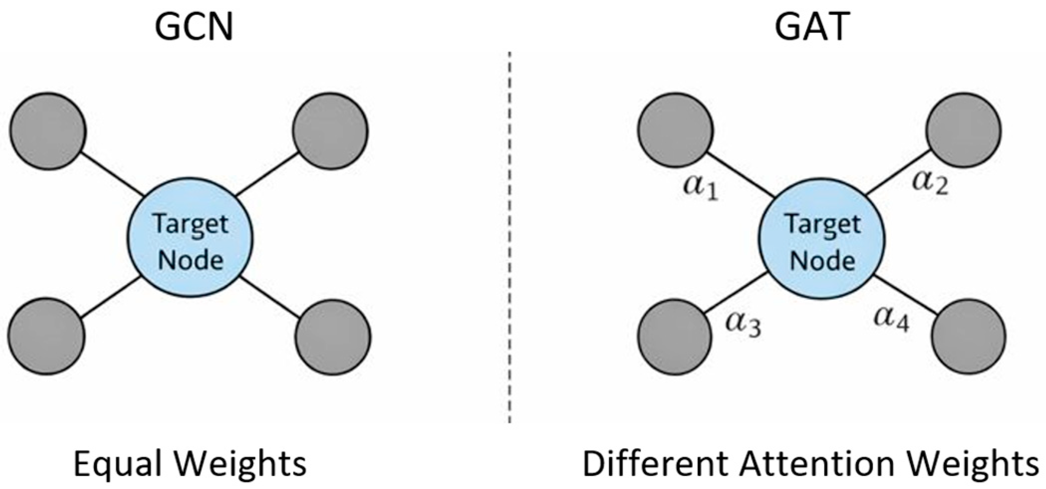
Graph attention networks (GAT) are an advanced architecture within the GNN family that introduces an attention mechanism into the process of information propagation among graph nodes. In contrast to conventional GCNs, which aggregate information from neighbors in a uniform manner (averaging), GATs learn a dynamic weight (attention score) for each edge. This enables the model to differentiate the influence that various neighboring nodes have on a given currency. The central concept behind GAT is that not all nodes adjacent to a given node are equally important. The attention mechanism allows the network to autonomously decide which neighbors are more critical, assigning them proportionally higher weights. The difference between uniform aggregation in GCN and attention-based aggregation in GAT is illustrated in Figure 1.

To better understand this mechanism, one can use an analogy of a social network. Imagine a group of friends where each person (node) is deciding on a weekend activity. While everyone provides suggestions, an individual does not value every friend’s opinion equally. They might pay more attention to a friend who is an expert in travel and less to someone who rarely goes out. In the GAT framework, the model acts like this individual: for a specific currency, it dynamically ‘listens’ more to the movements of currencies that are currently most relevant to its own price formation (e.g., a major trading partner), while assigning lower weights to others. This weighting is not fixed but changes based on the current market situation, much like a person might value a different friend’s advice when the topic changes from travel to finance.

Instead of treating all neighboring currencies as equally important, the model calculates a ‘relevance score’ for each pair. This score determines how much the information from a neighboring currency should influence the forecast of the target currency. In the context of modeling exchange rates, each node (currency) possesses a feature representation (e.g., log returns). This process proceeds through the following steps for every node $i$:

1.

Node Feature Transformation: The initial node features $x_i$ are transformed using a linear projection. This involves a weight matrix $W$ and results in a new feature representation:

$$h_i=W{x}_i$$

(2)

In practical terms, this transformation acts as a ‘feature filter.’ It projects the raw historical data into a higher-dimensional space where the model can more easily identify relevant patterns.

2.

Calculation of Raw Attention Coefficient: For every pair of connected nodes $(v_i,v_j)$ a raw attention coefficient ${ϵ}_{ij}$ is computed. This coefficient serves to evaluate the influence of node $v_j$ on node $v_i$. It is calculated by applying the attention weight vector $a$ to the concatenation of the transformed features of both nodes:

$${ϵ}_{ij}=\mathrm{L}\mathrm{e}\mathrm{a}\mathrm{k}\mathrm{y}\mathrm{R}\mathrm{e}\mathrm{L}\mathrm{U}\left(a^T\right[h_i‖h_j\left]\right)$$

(3)

This step evaluates the potential ‘importance’ of one currency to another. The raw coefficient represents an unrefined measure of influence; it asks: ‘How much should the price movement of currency j matter to currency i?’ This allows the model to consider the unique relationship between every pair of connected currencies in the network.

3.

Normalization of Attention Weights: To ensure the weights are comparable and sum to 1, the raw attention coefficients are normalized using the softmax function. The resulting attention weight ${\alpha }_{ij}$ shows the relative influence of neighbor $v_j$ on node $v_i$:

$${\alpha }_{ij}={\displaystyle \frac{\mathrm{e}\mathrm{x}\mathrm{p}\left({ϵ}_{ij}\right)}{{\sum }_{v_k\in \mathcal{N}\left(v_i\right)}\mathrm{e}\mathrm{x}\mathrm{p}\left({ϵ}_{ik}\right)}}$$

(4)

By using the softmax function, the model converts raw scores into percentages (weights). For instance, if the EUR ‘listens’ to three other currencies, this step might determine that 60% of its focus should be on the USD, 30% on the GBP, and 10% on the JPY.

4.

Information Aggregation: The new, aggregated representation of node $v_i$ is formed by the weighted sum of its neighbors’ representations, where the weights are the previously computed attention weights ${\alpha }_{ij}$:

$$h_i^{\prime }=\mathsf{\sigma }\left(\sum _{v_j\in \mathcal{N}\left(v_i\right)}{\alpha }_{ij}{h}_j\right)$$

(5)

where σ is an activation function (e.g., ReLU). In this manner, the node effectively ‘listens’ more intently to those neighbors that exert a greater influence on it. In this step, the architecture performs spatial information fusion. By summarizing weighted information from adjacent nodes, the model produces a comprehensive representation for each currency. This output accounts for both the individual currency’s performance and the significant cross-currency spillover effects identified by the attention mechanism.

In contrast to the fixed weights used in GCNs, the attention weights in GAT (${\alpha }_{ij}$) are dynamically learned during training and are entirely dependent on the features of the nodes. Consequently, even within a static graph structure, the attention weights can change based on the current market data.

GAT networks are highly versatile. They can operate effectively with both binary (unweighted) and weighted graphs, allowing for flexible modeling of diverse relationships between currencies. Furthermore, to enhance the model’s capacity to capture various types of dependencies, GAT often utilizes a multi-head attention architecture. Each attention head learns an independent set of weights and generates its own distinct node representation. The outputs from the individual heads are subsequently combined (e.g., through concatenation or averaging), which bolsters the model’s stability and predictive power. In our study, the initial layer employs 4 heads to capture diverse relationships, while the final layer reduces the number of heads to 1 to focus on the ultimate prediction.

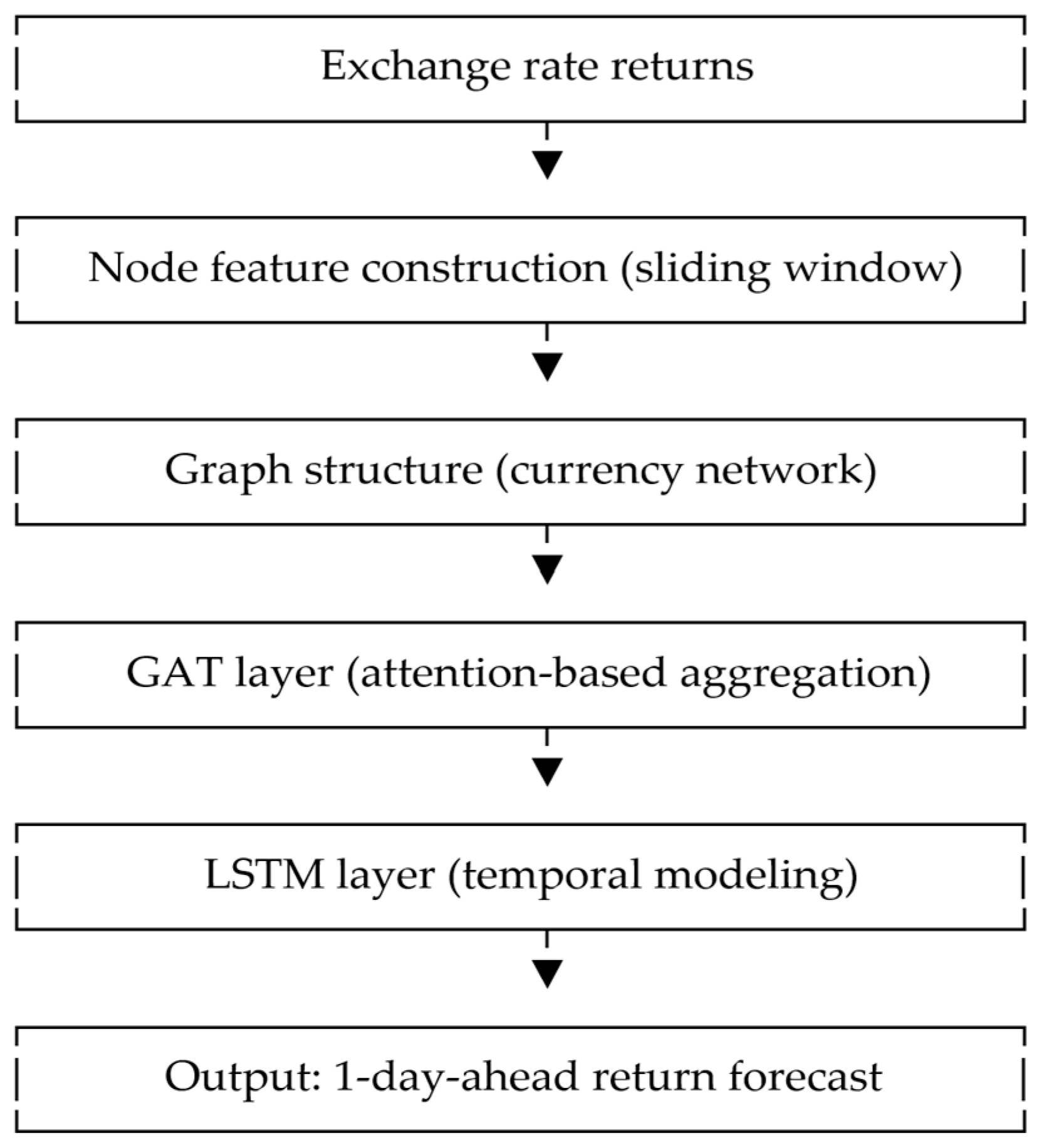
To enhance modeling capabilities, GAT can be integrated with other deep learning architectures. In the context of time series, a combination with Long Short-Term Memory (LSTM) networks is particularly useful. As a variant of RNNs, LSTMs are specifically designed to process sequential data. The key element of the LSTM is the cell state $c_v^{\left(t\right)}$, which functions as the network’s ‘memory’, enabling it to store information over long time intervals. In a hybrid LSTM-GNN architecture, the GNN component (e.g., GAT) is responsible for aggregating spatial information from the graph. It aggregates data from neighbors, factoring in their differentiated influence through the attention mechanism. Subsequently, this aggregated information is passed to the LSTM cell, which then updates the node’s hidden state over time. This combination allows the model to merge GAT’s ability to capture dynamic relationships between currencies (spatial information) with LSTM’s capacity to remember and process historical exchange rate data (temporal information). Such an integration facilitates the construction of more complex and accurate predictive models. The overall forecasting pipeline of the proposed model is summarized in Figure 2.

The training of GAT models utilizes a loss function that quantifies the difference between the model’s predictions and the actual observed values. In this study, the Mean Squared Error (MSE) was employed as the loss function, which heavily penalizes large errors due to the squaring operation.

$$L\left(y,\widehat{y}\right)={\displaystyle \frac{1}{n}}\sum _{i=1}^n{\left(y_i-{\widehat{y}}_i\right)}^2$$

(6)

Predictions are generated based on the learned embedding of the nodes, which represents their final, information-rich features:

$${\widehat{y}}_i=\varphi (z_i{W}_{out}+b_{out})$$

(7)

where $\varphi$ is a linear function, $z_i$ is the final node embedding, $W_{out}$ is the weight matrix, and $b_{out}$ is the bias. The final node embedding is a vector that encapsulates all information relevant to that specific node, which the model has gathered and processed up to the point of prediction. This embedding is a numerical vector that represents the currency in the feature space: it essentially summarizes the most critical information about the currency (its historical price, connections to others, i.e., information from its neighbors in the graph), and includes its ‘influence strength’ as seen in how much that currency changes the embeddings of its neighbors.

4. Data

The analysis utilized daily exchange rate data for 15 currencies against the New Zealand Dollar (X/NZD) for the period from 2 January 2020 to 31 December 2024 (1293 trading days), sourced from https://stooq.com. The selection of the time frame from January 2020 to December 2024 is intentional, as it provides a rigorous testing ground for the GAT model’s robustness during periods of extreme market regime shifts. This interval encompasses three major global shocks: the COVID-19 pandemic, the geopolitical crisis in Ukraine, and the subsequent global inflationary cycle with aggressive monetary tightening. By utilizing such a volatile period, we can effectively evaluate the GAT’s attention mechanism and its capacity to adapt to abrupt structural breaks and shifting inter-currency dependencies that static models often fail to capture.

The selection of 15 major currencies against the New Zealand Dollar (NZD) is based on their high global liquidity and economic significance. These currencies represent a broad spectrum of reserve (USD, EUR, GBP), regional (SGD), and commodity-linked (CAD) assets, ensuring a representative network for testing the GAT model. Furthermore, the NZD’s prominent role in global carry trade strategies makes it an ideal base currency for evaluating how the attention mechanism captures complex, time-varying interdependencies across diverse economic regimes. The list of currencies examined, along with their abbreviations and descriptive statistics, is presented in

Table 1. List of analyzed currencies with descriptive statistics.

Abbreviation	Currency Name	Mean	Standard Deviation	Range	Coefficient of Variation
CAD	Canadian Dollar	1.1807	0.0454	0.2301	0.0384
CHF	Swiss Franc	1.7068	0.1330	0.4972	0.0779
CNY	Chinese Yuan	0.2271	0.0075	0.0422	0.0329
EUR	Euro	1.7278	0.0639	0.3365	0.0370
GBP	Pound Sterling	2.0015	0.0800	0.3704	0.0400
HKD	Hong Kong Dollar	0.2005	0.0130	0.0568	0.0647
ILS	New Israeli Shekel	0.4489	0.0170	0.0943	0.0378
JPY	Japanese Yen	0.0124	0.0013	0.0060	0.1038
KRW	South Korean Won	0.0012	0.0000	0.0002	0.0326
NOK	Norwegian Krone	0.1601	0.0058	0.0261	0.0361
PLN	Polish Zloty	0.3840	0.0245	0.1156	0.0637
RUB	Russian Ruble	0.0203	0.0032	0.0206	0.1570
SEK	Swedish Krona	0.1597	0.0062	0.0291	0.0387
SGD	Singapore Dollar	1.1528	0.0735	0.2900	0.0637
USD	US Dollar	1.5635	0.1043	0.4539	0.0667

Source: Own calculations based on data from https://stooq.com.

.

The New Zealand Dollar (NZD), a currency of minor global significance, was chosen as the numéraire (base currency). The selection of an independent base currency is a complex issue for which no standard solution exists, and different choices may lead to varying results (see Basnarkov et al., 2019; Andrzejak et al., 2024).

The exchange rates were transformed into logarithmic returns according to the formula: $r_t=\mathit{log}\left(P_t/P_{t-1}\right)\times 100$. Stationarity of the time series is desirable during the network training phase, as it facilitates more reliable forecasting. Furthermore, to enhance the stability of the learning process, the logarithmic returns for each currency were normalized via standardization. This step is crucial in deep learning as it prevents larger-scale values from dominating and accelerates model convergence.

A time window of 30 days was used for modeling. This means that historical data from the preceding 30 days were utilized to forecast the logarithmic return for the subsequent day. To evaluate the model’s performance, the entire dataset was divided into three parts:

• Training Set: 70% of the data (883 observations), used for model learning;
• Validation Set: 15% of the data (189 observations), used for fine-tuning the model’s hyperparameters;
• Test Set: 15% of the data (190 observations), used for the final assessment of model performance. This set covered the period from 9 April 2024, to 31 December 2024, corresponding to 190 trading days.

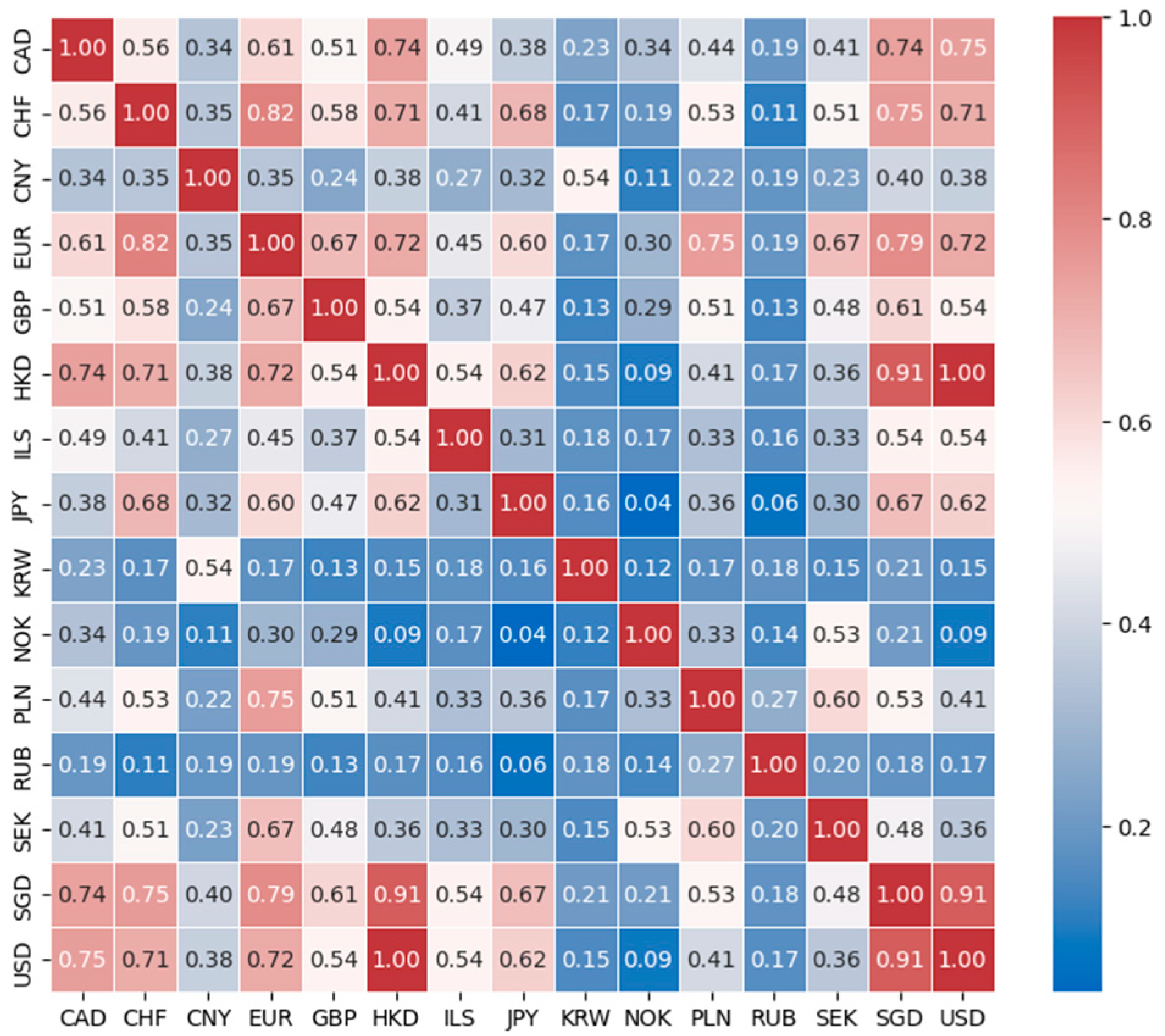
Figure 3 illustrates the correlation matrix of logarithmic returns for the examined currencies.

Figure 3 serves as the empirical foundation for constructing the currency network’s adjacency matrix. The heatmap reveals several distinct clusters of high positive correlation, particularly among major European currencies (e.g., EUR, CHF, and GBP). These strong dependencies justify the use of a graph-based approach, as they indicate that price movements in one node are significantly mirrored by its neighbors. Conversely, the varying intensity of colors illustrates the non-uniform nature of global currency relationships; for instance, the USD shows a more complex correlation pattern. By using these correlation coefficients as edge weights, our GAT model can prioritize information flow from the most statistically relevant neighbors, effectively filtering market noise during the forecasting process.

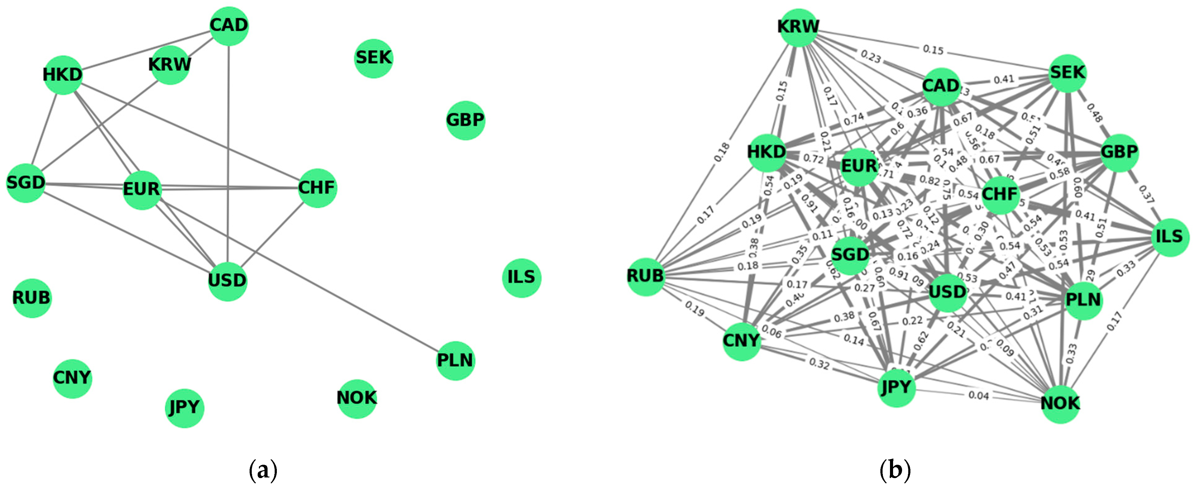
To conduct the analysis, a currency graph was constructed where the nodes represent the 15 selected currencies, and the edges reflect the dependencies between them. The edges were established based on the correlation of logarithmic returns. Two versions of the graph were tested in the experiments:

• Binary Graph: Edges existed if the correlation between the returns of two currencies exceeded a threshold of 0.7 (cf. Figure 4a);
• Weighted Graph: Edges were assigned weights equal to the actual correlation values (cf. Figure 4b).

5. Experiments

5.1. Comparison of Forecasting Results with Benchmarks

To assess the effectiveness of the proposed GAT architecture, a series of experiments was conducted, comparing its forecasting results against several benchmark models. The computations were performed in Python 3.10.0, leveraging libraries such as torch, torch_geometric, pandas, numpy, random, networkx, and scikit-learn. The analysis encompassed both classical statistical methods and modern neural network models. The primary research architecture applied was the GAT, including a hybrid variant integrated with LSTM networks (LSTM-GAT). The GAT models were constructed with several key components:

• GAT Layers: The networks consisted of two GAT layers, enabling the model to learn complex, hierarchical dependencies;
• Multi-Head Attention: Four attention heads were utilized, allowing for the simultaneous capture of diverse relationships among the currencies;
• Dropout: This technique was applied to randomly ‘switch off’ a portion of node features during training, which prevented model overfitting and improved generalization;
• Non-linear Activation: The ReLU activation function was applied after each GAT layer, introducing non-linearity to facilitate the learning of complex relationships.

The experiment differentiated between GAT models using a binary input graph and those using a weighted input graph. In the former case, the model receives a graph where edges are either ‘on’ (existing) or ‘off’ (non-existent). In the latter, the input graph provides pre-calculated weights (correlation values) that the GAT can use as additional information when learning its own attention weights. To evaluate the impact of the initial graph structure on the forecasting performance, we developed two variants for each model:

• Binary variant (_b): e.g., GAT_b, where the adjacency matrix is based on a binary threshold (0 or 1) of historical correlations;
• Weighted variant (_w): e.g., GAT_w, where the adjacency matrix incorporates the actual correlation values as initial edge weights.

In the final stage of network training, after passing through the GAT layers, each node obtained a final embedding, which was a combination of its own features and those of its neighbors, weighted by the attention mechanism. This representation was subsequently utilized to forecast the logarithmic return.

The results obtained from the GAT models were compared against the benchmarks:

• Naive Model;
• ARIMA Model;
• GARCH Model;
• Multilayer Perceptron (MLP);
• Convolutional Neural Network (CNN);
• Graph Convolutional Network (GCN): This model aggregates information from neighbors through simple averaging, lacking an attention mechanism;
• Hybrid LSTM-GCN Model: A combination of an LSTM network (for processing temporal sequences) and GCN (for graph processing).

The architecture and key parameters of the models used in the experiment are presented in

Table 2. Architecture and parameters of the models used in the experiment.

Model	Architecture	Number of Parameters
Naive	none	0
ARIMA	ARIMA(1,0,1), mi = 0	3 $\times$ 15 = 45
GARCH	GARCH(1,1), mi = 0	3$\times$ 15 = 45
MLP	num_features = 15, window = 30, 2 hidden layers, input_dim = 15∙30 = 450, hidden_dim = 32, output_dim = 15, ReLU activation, epochs = 50 (early stop 13), lr = 0.01, patience = 10	(15$\times$ 30$\times$ 32) + 32 + (32$\times$ 32) + 32 + (32$\times$ 15) + 15 = 15,983
CNN	num_nodes = 15, window = 30, 2 convolutional layers, 2 fully connected layers, hidden_cnn = 32, kernel_size = 3, ReLU activation, dropout = 0.2, epochs = 50 (early stop 20), lr = 0.005, patience = 10	(15$\times$ 32$\times$ 3) + 32 + (32$\times$ 15$\times$ 3) + 15 + (15$\times$ (30 − 4)) $\times$ 64 + 64 + (64$\times$ 15) + 15 = 28,926
GCN	num_nodes = 15, num_features = 30, 2 convolutional layers, hidden_gcn = 16, output_dim = 1, ReLU activation, dropout = 0.2, epochs = 50 (early stop 17), lr = 0.01, patience = 10	(30$\times$ 16) + 16 + (16$\times$ 1) + 1 = 513
LSTM-GCN	1 LSTM layer and 2 convolutional layers, hidden_lstm = 16, hidden_gcn = 16, output_dim = 1, ReLU activation, dropout = 0.2, epochs = 50 (early stop 11), lr = 0.01, patience = 10	4$\times$ 16$\times$ (1 + 16 + 1) + (16$\times$ 16) + 16 + (16$\times$ 1) + 1 = 1441
GAT_b	2 GAT layers, input_dim = 30, hidden_gat = 16, output_dim = 1, heads = 4, ReLU activation, dropout = 0.2, graph_mode = binary, thresh = 0.7, epochs = 50 (early stop 22), lr = 0.01, patience = 10	(30$\times$ 16$\times$ 4) + (16$\times$ 4) + (2$\times$ 16$\times$ 4) + (16$\times$ 4$\times$ 1$\times$ 1) + (1$\times$ 1) + (2$\times$ 1$\times$ 1) = 2179
GAT_w	2 GAT layers, input_dim = 30, hidden_gat = 16, output_dim = 1, heads = 4, ReLU activation, dropout = 0.2, graph_mode = weighted, epochs = 50 (early stop 22), lr = 0.01, patience = 10	((30 + 1) $\times$ 16$\times$ 4) + (16$\times$ 4$\times$ 2) + (2$\times$ 16$\times$ 4) + ((16$\times$ 4 + 1)$\times$ 1 $\times$ 1) + (1$\times$ 1$\times$ 2) + (2$\times$ 1$\times$ 1) = 2309
LSTM-GAT_b	2 LSTM layers and 2 GAT layers, hidden_lstm = 32, num_layers = 2, gat_hidden = 32, output_dim = 1, heads = 4, ReLU activation, dropout = 0.2, graph_mode = binary, thresh = 0.7, epochs = 50 (early stop 20), lr = 0.001, patience = 10	4$\times$ (1 + 32)$\times$ 32 + 4$\times$ 32 + 4$\times$ (32 + 32)$\times$ 32 + 4$\times$ 32 + (32$\times$ 32 + 32 + 2$\times$ 32)$\times$ 4 + (128$\times$ 1$\times$ 1) + (1$\times$ 1) + (2$\times$ 1$\times$ 1) = 17,283
LSTM-GAT_w	2 LSTM layers and 2 GAT layers, hidden_lstm = 32, num_layers = 2, gat_hidden = 32, output_dim = 1, heads = 4, ReLU activation, dropout = 0.2, graph_mode = weighted, epochs = 50 (early stop 17), lr = 0.001, patience = 10	4$\times$ (1 + 32)$\times$ 32 + 4$\times$ 32 + 4$\times$ (32 + 32)$\times$ 32 + 4$\times$ 32 + ((32 + 1)$\times$ 32 + 32$\times$ 2 + 2$\times$ 32)$\times$ 4 + ((128 + 1)$\times$ 1$\times$ 1) + (1$\times$ 1$\times$ 2) + (2$\times$ 1$\times$ 1) = 17,541

The suffixes _b and _w refer to the GAT models utilizing a binary and weighted input graph, respectively.

.

Table 2 details the architectural configurations and hyperparameter settings for all evaluated models. The choice of these parameters is informed by established practices in deep learning for financial time series (comp. Zhong et al., 2023). For instance, the use of 2 LSTM layers in LSTM-GAT model provides sufficient capacity to capture temporal dependencies without leading to rapid overfitting on noisy FX data. The ReLU activation function in the GAT layers was selected to mitigate the vanishing gradient problem, a standard approach in modern GNN literature (Veličković et al., 2017). Furthermore, the look-back window (input sequence length) was set to capture short-to-medium term market cycles, aligning with the methodology used by Xu et al. (2021) for high-frequency financial forecasting. This standardized configuration ensures that the performance gains observed in our hybrid models are attributable to their structural innovations rather than arbitrary parameter tuning.

As previously mentioned, to ensure a valid assessment of model performance, the return data were divided into three sets: training (70%), validation (15%), and test (15%). This partitioning was strictly chronological, simulating real market conditions where the model learns from historical data and verifies its effectiveness on newly emerging information (i.e., the test set). All predictive models generated one-day-ahead forecasts. This means that, based on data from a defined rolling time window, the model predicted the value for the single subsequent day. This process was repeated for every day in the test set, allowing for a comprehensive evaluation of model performance across the entire predictive horizon.

In order to establish a reliable, conservative baseline forecast, the GARCH(1,1) model was used. Based on a preliminary estimation, which showed that the estimated conditional mean is statistically insignificant and extremely close to zero (confirming the Efficient Market Hypothesis), the model was ultimately configured with a zero mean. This configuration is the most rigorous benchmark, forcing other models to prove their superiority in capturing dynamic market relationships.

In the case of the ARIMA model, it was estimated once on the training data, and then its parameters were ‘frozen’ and used in a loop to forecast subsequent test days. After each forecast, the model state was updated with new, actual observation.

All neural network models were trained using the Adam optimization algorithm. Among the baseline models, the LSTM-GCN served as a close benchmark for the proposed LSTM-GAT architecture. Their comparison enabled an isolated assessment of the influence of the attention mechanism on the final forecasting results, checking whether it genuinely improves predictive precision.

The evaluation metrics used to assess forecasting performance were the Mean Absolute Error (MAE) and the Mean Squared Error (MSE). The selection of these metrics is dictated by their complementary nature. MAE, in contrast to MSE, treats all errors linearly, which makes it robust against the influence of extreme observations (outliers). Conversely, MSE heavily penalizes large errors, causing models that minimize MSE to strive for avoiding significant deviations from actual values. Both metrics were calculated globally (for all currencies combined) and separately for each currency, allowing for an asset-specific analysis of model performance.

Table 3. Average 1-day forecast errors for returns on the test set.

Model	MAE	MSE
Naive	0.589831	0.699702
ARIMA	0.419779	0.354605
GARCH	0.417343	0.351605
MLP	0.419828	0.355416
CNN	0.419100	0.353761
GCN	0.421377	0.358629
LSTM-GCN	0.418693	0.352437
GAT_b	0.419229	0.353282
GAT_w	0.428371	0.370248
LSTM-GAT_b	0.418660	0.353307
LSTM-GAT_w	0.418745	0.353689

The four lowest error values for both MAE and MSE are highlighted in bold.

presents the average 1-day forecast errors for returns on the test set.

Among all tested models, the four best results were achieved by the GARCH, LSTM-GCN, LSTM-GAT_b, and LSTM-GAT_w models. Notably, the hybrid models combining GNNs with LSTM (LSTM-GCN, LSTM-GAT_b, LSTM-GAT_w) demonstrated exceptionally low errors, placing them at the top of the ranking. Their performance is comparable to that of the best statistical model (GARCH). This suggests that LSTM’s capability to model time series, combined with the GNN’s ability to capture dynamic inter-currency dependencies, is crucial for significantly increasing forecasting precision.

The observation that the basic GARCH(1,1) model, particularly when configured with a zero conditional mean, achieves forecasting errors (MSE and MAE) that are highly competitive with, or even superior to, the complex LSTM-GAT architectures warrants a crucial discussion. This outcome is consistent with the Efficient Market Hypothesis, which posits that exchange rates exhibit near-random walk characteristics. The fact that the estimated non-zero constant mean in the GARCH model is empirically indistinguishable from zero confirms the strong form of market efficiency in predicting the mean return. Consequently, the performance of classical linear models establishes a robust, theoretically grounded market benchmark, proving the difficulty of obtaining a statistically significant predictive edge in forecasting the value of the exchange rate return itself.

The GAT models, particularly the one utilizing the binary graph (GAT_b), achieved very strong results, thus confirming the effectiveness of the attention mechanism in prediction. An interesting observation is the minimal difference between the LSTM-GAT_b model (MAE = 0.418660) and LSTM-GAT_w (MAE = 0.418745), which indicates that adding input weights (GAT_w) did not yield a significant improvement compared to the simpler, binary approach. This fact, coupled with the higher error values observed in the GAT_w model, may suggest that the attention weights generated internally by the model itself are more adequate than those initially imposed a priori.

The empirical results indicate that weighted graphs do not improve prediction quality relative to binary graphs. This outcome underscores an important insight: static correlation-based weights may not reflect rapidly changing FX relationships. GAT attention mechanisms dynamically infer optimal weights from the data, rendering externally imposed weights less effective. This affirms the advantage of allowing the architecture to autonomously learn dependency strengths.

The top-performing models surpassed the GCN, CNN, and MLP benchmarks, underscoring the importance of incorporating graph structure and dynamic attention in the analysis of currency markets. The GCN and GAT_w models registered distinctly higher errors, which may signify that both the absence of an attention mechanism (GCN) and the imposition of predefined weighted connections (GAT_w) negatively affect the model’s ability to adapt to dynamically changing market conditions.

5.2. Forecasting Results for Individual Currencies

Table 4. Average 1-day forecast errors for individual currencies on the test set obtained from the LSTM-GAT_b model.

Currency	MAE	MSE
CAD	0.344229	0.187115
CHF	0.392264	0.250695
CNY	0.369795	0.235781
EUR	0.317761	0.160647
GBP	0.310959	0.159891
HKD	0.438469	0.325966
ILS	0.546127	0.466346
JPY	0.521049	0.467863
KRW	0.363379	0.219205
NOK	0.325627	0.15619
PLN	0.379758	0.231868
RUB	0.867362	1.705885
SEK	0.329075	0.186000
SGD	0.328826	0.211675
USD	0.445226	0.334482

For both MAE and MSE, the three lowest error values are presented in bold, and the three highest error values are presented in italics.

presents the averaged 1-day forecast errors for each individual currency, calculated on the test set using the LSTM-GAT_b model, which was shown in the previous section to be one of the most effective architectures. An analysis of these results allows us to identify which currencies are the easiest and which are the most difficult for the model to predict.

The LSTM-GAT_b model achieved the lowest MAEs and MSEs for currencies such as GBP, EUR, NOK, SGD, and SEK. Both the GBP and EUR are well-established market currencies whose returns are characterized by relatively stable dynamics compared to other assets. The model’s ability to precisely model these currencies may stem from their strong outgoing influence on other network currencies. The low errors for NOK and SEK indicate that the model performs well with the Scandinavian currencies.

Conversely, the model recorded the highest errors for RUB, ILS, and JPY. These currencies were clearly the most challenging to forecast. The extremely high errors for the RUB are not surprising. The Ruble is known for its high volatility and susceptibility to geopolitical factors, which makes it exceptionally difficult to predict. Its returns are likely based on a fundamentally different dynamic that lies outside the model’s scope. High errors for the ILS and JPY also suggest that their unique specificities and reactions to macroeconomic and geopolitical factors pose a significant challenge to the algorithm. In the case of the Japanese Yen, this difficulty may be attributed to the specific policies pursued by the Bank of Japan, which differentiate it from other major currencies.

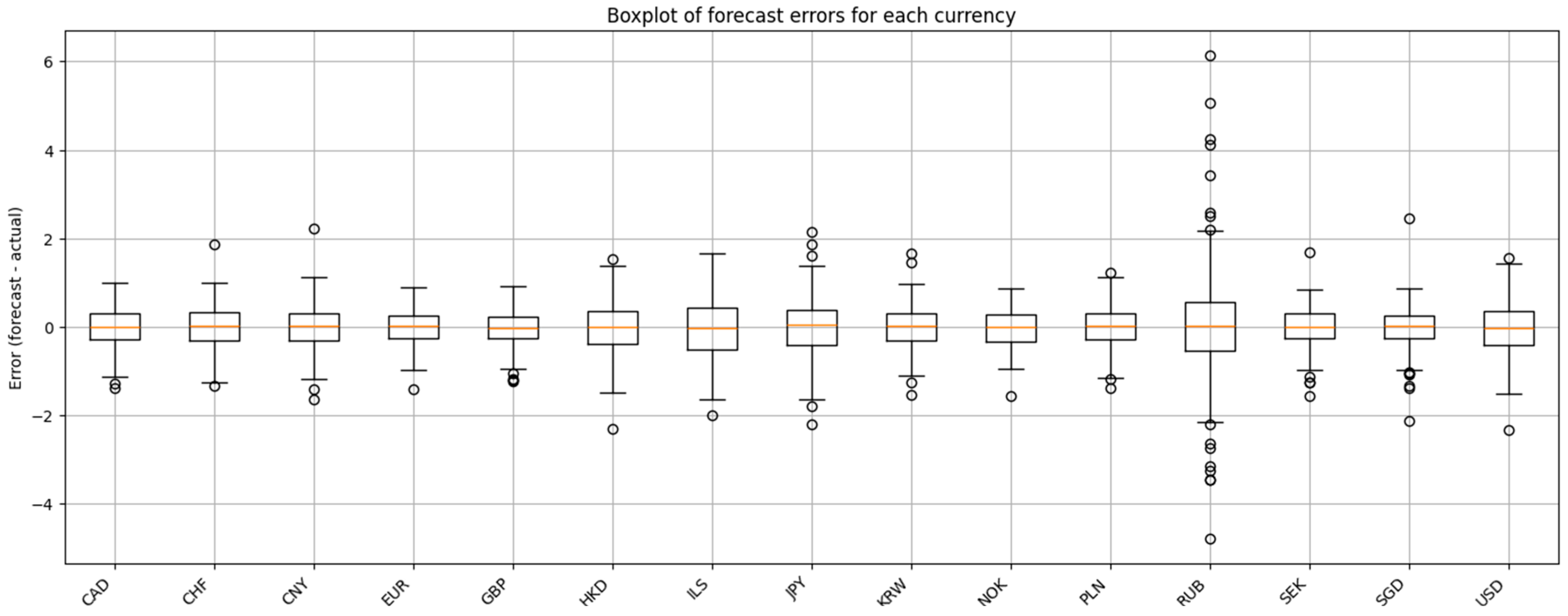
The analysis of the forecast error distribution, conducted using box plots (Figure 5), allows for an assessment of the forecast characteristics for each currency, particularly for identifying the dispersion (spread) and the presence of extreme values (outliers) within the error distribution.

The analysis of the error distribution confirmed the conclusions drawn from the table of average errors. For instance, an exceptionally large number of outliers was observed for the Russian Ruble (RUB), indicating that the LSTM-GAT_b model had significant difficulty accurately forecasting its returns during critical periods. A large dispersion (spread), visible in the length of the box plot ‘whiskers’ and the size of the box itself, was also characteristic of the ILS and USD. Conversely, currencies such as the EUR and GBP featured a much more compact error distribution and fewer outliers, which supports their stability and predictability for the model.

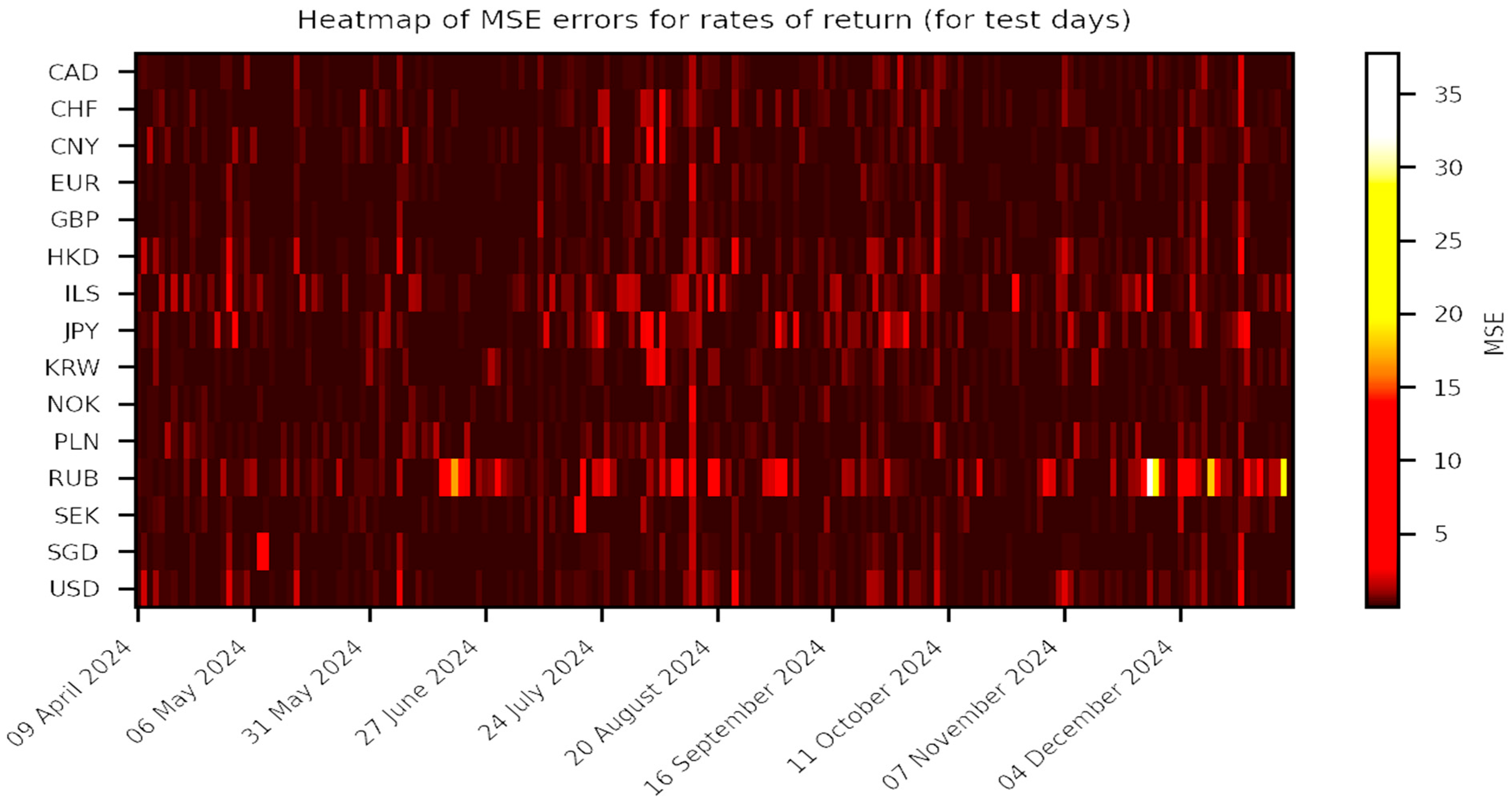
A heatmap of MSEs as a function of currency and day (Figure 6) allows for the identification of specific currencies and time periods that were particularly challenging to forecast.

In contrast to the table of average errors, which provides aggregated values, the heatmap reveals the dynamics and specific moments when the model encountered the greatest difficulties. The chart clearly demonstrates that the model had the most significant problems forecasting the Russian Ruble (RUB). The bright, horizontal bands in the RUB row indicate that errors for this currency were consistently high, and at certain points represented by the intense yellow color, extremely high (e.g., in June 2024, the US imposed sanctions on the Moscow Exchange (MOEX) and the National Clearing Center (NCC), and at the end of 2024, there was a ‘black November for the Russian economy’ when sanctions led to a 50% depreciation of the RUB against the USD). Specific periods where the model performed poorly in forecasting multiple currencies simultaneously can also be identified. Visible vertical bright bands appear, particularly around mid-August and December. This may suggest the occurrence of unforeseen macroeconomic factors that affected overall market volatility.

6. Discussion

The conducted study demonstrates that hybrid models based on the GAT architecture, particularly when combined with LSTM networks, achieve exceptionally high efficacy in forecasting currency return time series. The results of the LSTM-GAT_b and LSTM-GAT_w models, as measured by the averaged MAEs and MSEs, place them on par with the most effective statistical model tested, GARCH. This conclusion is consistent with the increasing trend in the scientific literature that points to the advantage of GNNs in tasks involving the modeling of complex dependencies in financial data. Research by authors such as Wu et al. (2021) and Kipf and Welling (2017) confirms that GNNs are capable of capturing sophisticated spatio-temporal dependencies, which leads to an improvement in forecast quality compared to traditional models like ARIMA or GARCH.

Our findings specifically highlight how the attention mechanism serves as a bridge between pure statistical forecasting and financial reality. The novelty of our implementation is demonstrated by the model’s ability to maintain high predictive accuracy even when the underlying market correlations are non-linear and asymmetric. While traditional methods suffer from ‘parameter lag’ when market regimes change, the GAT-based framework adapts its attention weights instantly based on the current market state. This means the model does not just aggregate data; it intelligently selects which information is most relevant at any given moment, effectively capturing the current dynamics of the FX network in a way that traditional linear and static models cannot replicate.

Our results have interesting implications when viewed through the lens of the Efficient Market Hypothesis (EMH). According to the weak form of EMH, all past price information is already reflected in current prices, making it impossible to achieve superior returns through technical analysis or historical data modeling. However, the high forecasting accuracy of our GAT-based models suggests that the FX market may not be perfectly efficient in its weak form. The success of the attention mechanism indicates that there are complex, non-linear dependencies and ‘lead-lag’ relationships between currencies that traditional models fail to capture. By dynamically weighing the influence of neighboring nodes, the GAT model identifies patterns of information diffusion across the currency network that occur over time. This aligns with the Adaptive Market Hypothesis (AMH), which suggests that market efficiency is not a static state but an evolving process.

The EMH suggests that one-step-ahead returns behave nearly as a martingale difference sequence, limiting the achievable predictive edge. Therefore, the fact that LSTM-GAT achieves performance comparable to GARCH confirms that the model has successfully captured the available signal without overfitting. The value-added dimension of GAT lies in its structural representation: it extends forecasting analysis beyond temporal prediction and into the domain of network-based financial interpretation.

The advantages of hybrid network models have been previously emphasized in the literature, and these architectures similarly achieved strong performance in our study. Specifically, the effective integration of LSTM with GCN has been successfully implemented by several researchers across various financial domains. For example, C. Liu and Paterlini (2023) presented a method for forecasting stock returns based on the LSTM-GCN model. Their model, trained on datasets representing the Eurostoxx 600 and S&P 500 indices, demonstrated that the inclusion of spatial information (i.e., relationships between companies) enhanced predictability, outperforming standard benchmarks. Similarly, Shi et al. (2025) utilized an LSTM-GCN architecture, where the GCN captured spatial relationships between stocks and the LSTM modeled temporal return dynamics. Tested across the DJIA, SSE50, and CSI100 indices, their model achieved superior metrics (lower MSE and MAE, and better R2) compared to competing models (such as LSTM, GCN, and GRU). For instance, they reported an MSE of approximately 0.0055 and an R2 between 0.89 and 0.92 for the DJIA. Further, Sonani et al. (2025) created a hybrid LSTM-GNN model where the GNN component modeled inter-stock dependencies while the LSTM handled temporal dynamics. This synergistic combination resulted in a significantly better MSE, showing a 10.6% decrease in error compared to a standalone LSTM model, and better results than linear regression, CNN, and dense networks. The conclusion across these studies is clear: combining a GNN as a spatial layer with LSTM as a temporal layer is highly effective. Finally, Foroutan and Lahmiri (2024) applied an ST-GNN, confirming that the attention mechanism effectively improved forecast accuracy. They showed that ST-GNN models outperform standard deep learning methods (like CNNs, LSTMs, and TCNs). It is worth noting that their methodology is easily transferable to FX problems.

Our study focused directly on the FX market. Although analyses applying these advanced network models to this area are scarce in the existing literature, the work of Guan and Ge (2024) serves as a valuable comparative reference. The authors constructed a currency graph-based model, the ST-GAT, utilizing a GAT layer to capture spatial dependencies and a Transformer block to process temporal dynamics. Their results, on a dataset covering 17 major currencies over 2092 trading days, demonstrated that the ST-GAT surpasses classical LSTM and GCN in terms of MSE and directional accuracy. Furthermore, their STGAT model with a hierarchical transformer outperformed both standard ST-GNNs and classic sequential models. This provides compelling evidence that graph attention is directly beneficial in FX forecasting, a conclusion strongly supported by our own findings regarding the validity of utilizing the attention mechanism.

One of the greatest strengths of the GAT model is its ability to reveal complex, asymmetric relationships between currencies. In contrast to traditional models based on static correlation, GAT generates attention weights that are dynamic and can evolve over time. Our particularly interesting finding is the fact that the model with the binary graph (GAT_b) achieved results no worse than the model with the weighted graph (GAT_w). This suggests that the flexibility to independently learn attention weights, rather than imposing them a priori, is a key advantage of the model. Instead of relying on static, predefined measures (like correlation), the GAT model is able to autonomously develop optimal connections. The observed superiority of GNN models over simpler architectures like MLP and CNN unequivocally underscores that incorporating graph structure and the dynamic attention mechanism constitutes a fundamental advantage in financial market analysis.

While classical models such as GARCH achieve highly competitive performance in forecasting FX returns, the objective of this study was not to surpass these benchmarks in error metrics. Instead, the goal was to assess whether graph-based architectures—particularly GAT and hybrid LSTM-GAT models—can offer predictive accuracy comparable to traditional econometric models while providing additional structural insights unavailable in ARIMA or GARCH frameworks. In contrast to linear models focused solely on temporal dynamics, GAT-based models learn asymmetric, dynamic inter-currency dependencies represented through attention weights. These weights reveal evolving influence patterns that enhance interpretability of the global FX network.

7. Conclusions

To understand the significance of this study for the broader financial market, it is helpful to view the global currency exchange as a ‘living network’ rather than a set of isolated numbers. Traditionally, forecasting models look at one currency’s past to predict its future. Our research shifts this perspective by showing that currencies ‘talk’ to each other; an event in one corner of the globe sends ripples through the entire network. By using GAT networks, we have essentially created a dynamic map that tracks these invisible connections in real-time. This approach allows us to see not just how much a rate might change but why, by identifying which other currencies are currently driving that movement. For the non-technical reader, the key takeaway is that our model provides a more intuitive and ‘human-like’ way of understanding market interdependencies, offering a clearer picture of global financial stability.

Building on this intuition, our empirical analysis provides direct answers to the research questions posed in this study. Regarding Q1, we have validated the high utility of hybrid forecasting models, demonstrating that the LSTM-GAT architecture constitutes a structurally superior framework compared to standard deep learning methods and traditional benchmarks. While the GARCH model remains highly competitive in terms of MSE, the hybrid GNN-based approach offers a more comprehensive analytical depth. In response to Q2, our results confirm that integrating attention-based spatial dependencies significantly improves the model’s capacity to capture dynamic and asymmetric relationships between currencies, which is a clear advantage over models that ignore network interconnectedness. Finally, addressing Q3, our experiments indicate that weighted graph structures (_w) provide a more nuanced foundation for the attention mechanism than simple binary networks (_b), as they allow the model to leverage prior information about correlation strengths to better prioritize relevant neighbor influences.

The results obtained in this study have several concrete implications for real-world financial practice. From the perspective of short-term trading strategies, the proposed LSTM–GAT framework may serve as a decision-support tool by identifying currencies whose short-horizon returns are relatively more predictable due to their stable position within the FX network (e.g., EUR or GBP). Conversely, currencies characterized by rapidly changing or highly volatile attention patterns (such as RUB or ILS) may indicate elevated uncertainty, suggesting the need for reduced exposure, tighter stop-loss rules, or higher risk premiums.

In the context of portfolio management, the dynamically learned attention weights offer information that goes beyond static correlation matrices typically used in currency diversification. By capturing time-varying and asymmetric inter-currency dependencies, the GAT-based model can help portfolio managers detect periods when diversification benefits weaken due to increasing network interconnectedness, thereby supporting more adaptive allocation and hedging decisions.

Finally, from a macro-financial and policy perspective, the attention mechanisms embedded in the GAT architecture provide a novel way to monitor shifts in global currency influence and spillover intensity. Central banks and financial authorities could potentially use such models as complementary monitoring tools to identify emerging dominance structures or heightened systemic interconnectedness in the FX market, particularly during periods of financial stress.

However, the limitations of these sophisticated models must be acknowledged. They suffer from high computational complexity and implementation costs, particularly for ST-GAT architectures dealing with many currency pairs and short time intervals. Crucially, the inherent non-stationarity of financial markets—where relationships can change abruptly (e.g., correlations breaking during crises)—requires continuous graph adaptation. Finally, the frequent omission of real-world constraints like transaction costs (spread, slippage, liquidity limits) in academic evaluation limits the realism of reported results, often inflating perceived performance.

Despite these challenges, the potential of GNNs in financial market analysis is immense. Future research could further enhance the model’s accuracy by addressing several key areas. First, the framework could be extended to include real-time adaptation, allowing the attention weights and network structure to update instantaneously as new market data arrives. Second, incorporating external data sources, such as news sentiment, social media trends, or geopolitical event indicators, would provide the model with a multi-modal context that numerical price data alone cannot capture. Furthermore, rigorous comparative studies between GAT and Transformer-based hybrids are needed to precisely determine the advantage of graph-based spatial insights over purely temporal attention models. Finally, continued efforts should be directed toward developing techniques that improve the interpretability of these models, showing more clearly how the graph perspective explains the underlying drivers of financial market movements.