Simple Approximations and Interpretation of Pareto Index and Gini Coefficient Using Mean Absolute Deviations and Quantile Functions

Abstract

The Pareto distribution has been widely used to model income distribution and inequality. The tail index and the Gini index are typically computed by iteration using Maximum Likelihood and are usually interpreted in terms of the Lorenz curve. We derive an alternative method by considering a truncated Pareto distribution and deriving a simple closed-form approximation for the tail index and the Gini coefficient in terms of the mean absolute deviation and weighted quartile differences. The obtained expressions can be used for any Pareto distribution, even without a finite mean or variance. These expressions are resistant to outliers and have a simple geometric and “economic” interpretation in terms of the quantile function and quartiles. Extensive simulations demonstrate that the proposed approximate values for the tail index and the Gini coefficient are within a few percent relative error of the exact values, even for a moderate number of data points. Our paper offers practical and computationally simple methods to analyze a class of models with Pareto distributions. The proposed methodology can be extended to many other distributions used in econometrics and related fields.

1. Introduction

The Pareto distribution Pareto (1897) is commonly used for modeling income inequality Coelho et al. (2008) due to its heavy-tailed nature, capturing wealth concentration Bennett et al. (2019); Brzezinski (2014); Catalano et al. (2009); Chotikapanich et al. (2007); Pinsky et al. (2024). The tail index $\alpha$ and Gini coefficient G are key parameters Catalano et al. (2009); Gini (1912, 1936). Traditional methods like maximum likelihood Beirlant et al. (1996); Grimshaw (1993); Rytgaard (1990) and the method of moments are sensitive to outliers and can fail when moments do not exist Beirlant et al. (1996); Hill (1975). Recent literature has turned to quantile-based methods for their robustness and applicability to heavy-tailed distributions Brazauskas and Serfling (2007); Pickands (1975). However, existing quantile and moment estimators often involve complex calculations or require multiple quantiles Chotikapanich et al. (2007); Dekkers et al. (1989); Hussain et al. (2018). A comparison of recent methods for parameter estimation for the Pareto distribution is presented in Warsono et al. (2019).

This paper presents a simple method for estimating $\alpha$ and G using only the first quartile $Q_1$, median M, and third quartile $Q_3$. Our approach uses the mean absolute deviation (MAD) Bloomfield and Steiger (1983) and truncation to estimate and interpret the parameters in terms of the corresponding sub-areas computed as integrals of the underlying quantile function. Our approximation formulas directly yield simple closed-form formulas relating the tail index and the Gini coefficient to quartiles. The proposed MAD-based method is robust (50% breakdown point), making it ideal for heavy-tailed data Hampel (1974) with outliers often present in income and wealth distributions data Bennett et al. (2019); Brzezinski (2014).

One of our main results is the approximation of the tail index $\alpha$ and the Gini coefficient G using the median and weighted average of the other two quartiles. By considering different quadrature approximation methods, we obtain different weights and a number of approximations to the parameters. For example, in one such approximation, the tail index $\alpha$ is shown to be half the inverse Bowley–Galton skewness coefficient Bowley (1920), and the Gini index G is one-half of the ratio of the quartile difference to the lower quartile difference. These approximations allow us to connect classical quantile statistics Huber (2009) and Pareto parameters. Our approach offers several advantages:

• Computational simplicity—order statistics readily available from standard software;
• Applicability to truncated distributions (e.g., income surveys with top-coding);
• Elegant geometric and economic interpretation via areas under the quantile function and income groups.

This paper is organized as follows. In Section 2, we introduce the Pareto distribution and discuss its quantile function. In Section 3, we derive and interpret mean absolute deviation for a continuous distribution in terms of the subareas of the quantile functions. In Section 4, we apply these ideas to the Pareto distribution. In Section 5, we interpret the indices in terms of the ratio of the appropriate subarea integrals. In Section 6, we provide an economic interpretation of these indices. In terms of a truncated Pareto distribution. In Section 7, we consider the truncated Pareto distribution and derive its mean absolute deviation. This will allow us to express the tail index $\alpha$ and the Gini coefficient in terms of quartiles and, at the same time, address the practical issue of dealing with outliers in real data sets. In Section 8, we derive an approximation to indices using the mean absolute deviation of a truncated distribution. By contrast, in Section 9, we derive several approximations to these indices using the mean of the truncated distributions and several integral quadrature methods. The proposed approximations have simple geometric and economic interpretations. The obtained formulas are expressed in terms of very simple expressions involving the median and weighted average of the other two quartiles. In Section 10, we provide a summary of the proposed approximation formulas. In Section 11, we summarize our proposed estimation formula and compare it to the Maximum Likelihood Estimation. In Section 12, we present simulation results to illustrate our approach. These simulations show that the proposed estimators achieve relative errors within a few percent of true values for even small sample sizes. In Section 13, we illustrate our approximations on several real datasets. Finally, in Section 14, we present some concluding remarks and discuss future directions.

In this paper, we focus on income inequality. Many economists focus on other components of income, such as wages and earnings, or on some utility functions like consumption and leisure Attanasio and Pistaferri (2016). We do not advocate a particular viewpoint on established theories in finance and economics (permanent income hypothesis, lifecycle models, wealth accumulation, and others). Our objective is to show that the proposed formulas for the Pareto distribution allow for the derivation of simple economic interpretations in terms of quantile-based metrics. We emphasize that these approximations do not require full knowledge of the underlying distributions. Since the obtained metrics are available in closed form in terms of simple quantile measures, one can study the effect of changes by examining the differences in quantiles over time. This allows for the application of the proposed methodology to time-varying or dynamic quantile models. Therefore, our methodology and formulas are general and can be used to interpret other models described by the Pareto distribution.

2. Pareto Distribution

Suppose X is distributed according to the Pareto distribution Feller (1956); Johnson and Kotz (1970); Papoulis (1984) over the domain $x\ge \beta$ with scale $\beta >0$ and shape $\alpha >0$. Its density $f\left(x\right)$ and its cumulative distribution function $F\left(x\right)$ are given by

$$f\left(x\right)={\displaystyle \frac{\alpha {\beta }^{\alpha }}{x^{\alpha +1}}}\mathrm{and}F\left(x\right)=1-{\left({\displaystyle \frac{\beta }{x}}\right)}^{\alpha }$$

(1)

For this distribution, no moments exist for $\alpha \le 1$ Arnold (2015). The first moment is finite for $\alpha >1$, and the second moment exists only for $\alpha >2$. The mean $\mu$ and variance ${\sigma }^2$ for this distribution are

$$\mu ={\displaystyle \frac{\alpha \beta }{(\alpha -1)}}\mathrm{for}\alpha >1\mathrm{and}{\sigma }^2={\displaystyle \frac{\alpha {\beta }^2}{{(\alpha -1)}^2(\alpha -2)}}\mathrm{for}\alpha >2$$

(2)

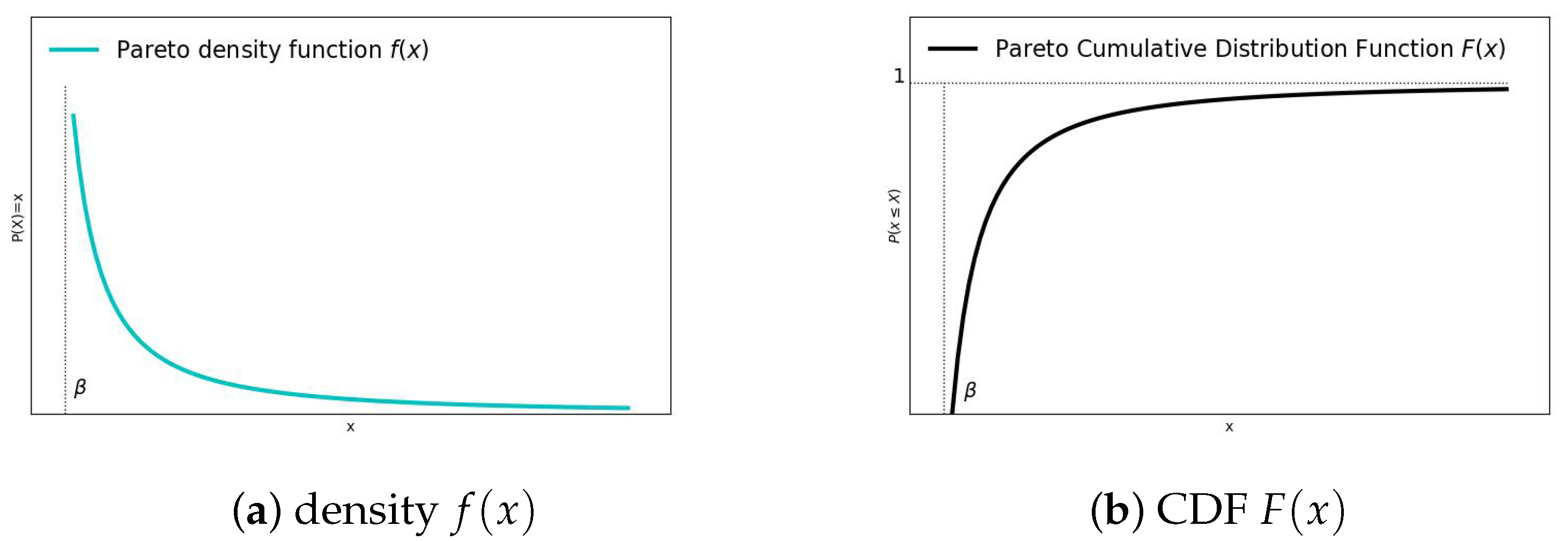
Of practical interest is the case $\alpha >1$. For example, many datasets have $\alpha$ in the range $1<\alpha <2$ Dallas (1976). Pareto density $f\left(x\right)$ and cumulative distribution function $F\left(x\right)$ are illustrated in Figure 1.

The Pareto distribution is right-skewed, with more data points on the lower end Dallas (1976); MacGillivray (1986). In economic terms, this can be interpreted as stating that lower-income people have a disproportionately lower share of the total wealth.

Let $Q\left(p\right)$ be the quantile function defined by $Q\left(p\right)=inf\{x:F(x)\ge t\}$ with $t\in [0,1]$. For the Pareto distribution, the quantile function is Gilchrist (2000)

$$Q\left(p\right)=\beta {(1-p)}^{-1/\alpha }$$

(3)

and therefore, for the quartiles $Q_1$, $Q_2=M$, and $Q_3$ we have

$$Q_1=\beta {(4/3)}^{1/\alpha },M=\beta 2^{1/\alpha }\mathrm{and}{Q}_3=\beta 4^{1/\alpha }$$

(4)

Since $\alpha >1$ and $0\le p\le 1$, for the first and second derivatives of $Q\left(p\right)$, we have

$$Q^{\prime }\left(p\right)={\displaystyle \frac{Q\left(p\right)}{\alpha (1-p)}}>0\mathrm{and}{Q}^{″}\left(p\right)={\displaystyle \frac{(\alpha +1)Q\left(p\right)}{{\alpha }^2{(1-p)}^2}}>0$$

(5)

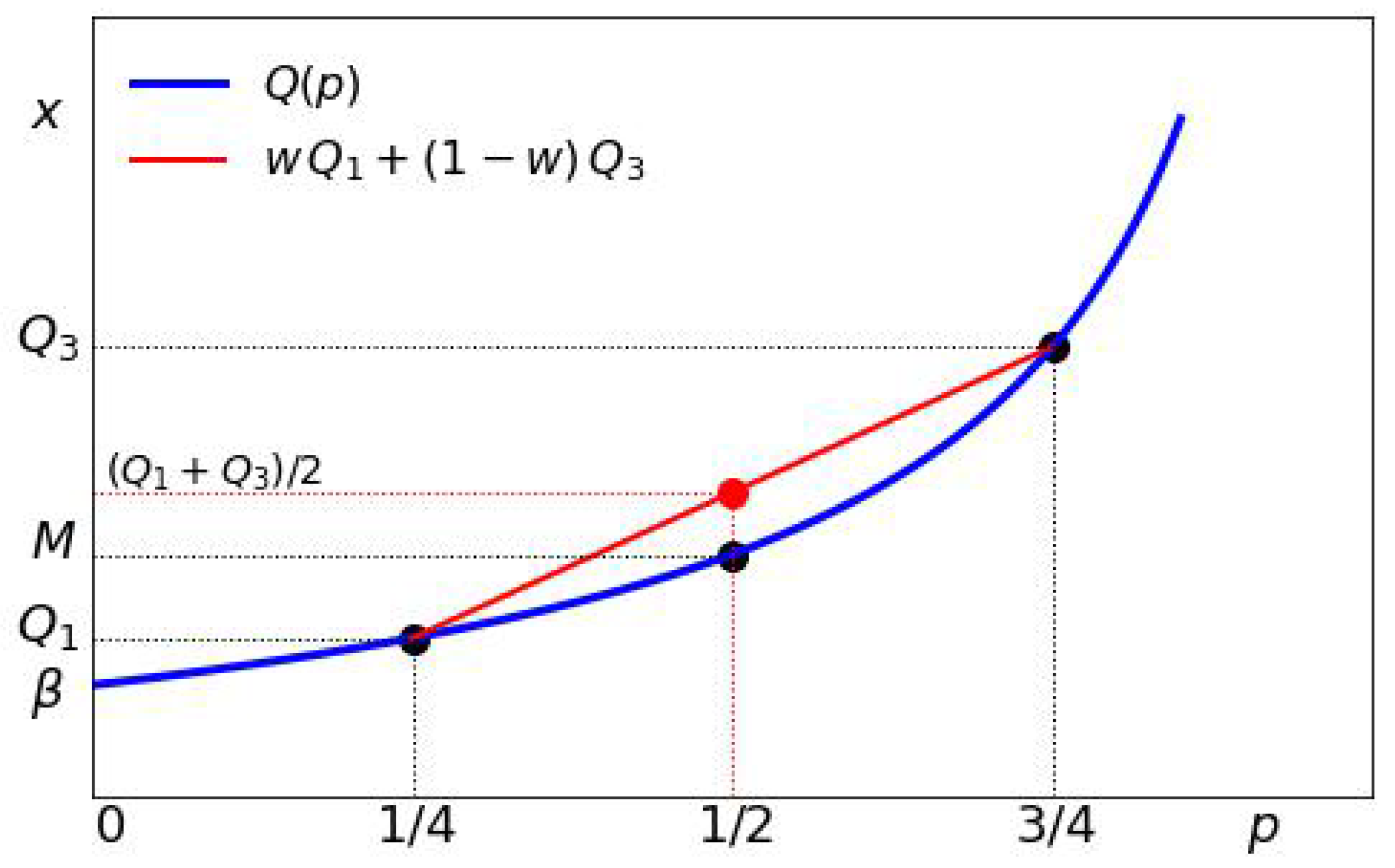
and therefore, the quantile function $Q\left(p\right)$ is an increasing convex function with a minimum $Q\left(0\right)=\beta$. It follows then that for any $0\le p_1<p_2\le 1$ and any $0\le w\le 1$ we have $wQ\left(p_1\right)+(1-w)Q\left(p_2\right)>Q\left(w{p}_1+(1-w)p_2\right)$. This is illustrated in Figure 2.

In Figure 2, we take $p_1=1/4$, $p_2=3/4$, and $w=1/2$. The convexity of $Q\left(p\right)$ implies that $M<(Q_1+Q_3)/2$. We may consider other choices for $p_1$, $p_2$, and w and obtain the following inequalities that will be useful later in this paper:

• $w=1/3$:  $\beta /2+2Q_3/3>Q_1$
• $w=1/2$:  $\beta /2+M/2>Q_1$ and $Q_1/2+Q_3/2>M$
• $w=2/3$:  $2\beta /3+Q_3/3>M$

3. Mean Absolute Deviation

Let us start by outlining our methodology. It is based on using mean absolute deviations to derive simple expressions for the tail index and the Gini coefficient as an alternative to the traditional approach of deriving them, mainly the maximum likelihood estimation. Using mean absolute deviation is a standard statistical technique of estimating parameters that minimizes the calculated mean absolute deviation. Specifically, we derive mean absolute deviations in terms of the integrals of the quantile function. With simple quadrature approximations to these integrals, we express metrics of interest in terms of simple expressions involving the quartiles. This allows a simple explanation of the results in terms of the quantile metrics.

The proposed approximations do not require the full knowledge of the underlying distribution. The main attractiveness of the proposed method is its simplicity—we express our results in terms of the weighted averages of the quartiles.

Let us start with mean absolute deviations. Suppose X is a real-valued random variable with density $f\left(x\right)$ and cumulative distribution function $F\left(x\right)$. Let $Q\left(p\right)$ be the quantile function defined by $Q\left(p\right)=inf\{x:F(x)\ge t\}$ with $t\in [0,1]$. Let $Q_1$, $Q_2=M$, and $Q_3$ denote the first quartile, median, and third quartile, respectively.

If X has a finite first moment $\mu$, then for any value a we can define the mean absolute deviation H of X around the a by Bloomfield and Steiger (1983).

$$H\left(a\right)=\int |x-a|f\left(x\right)dx={\int }_{x\le a}(a-x)f\left(x\right)dx+{\int }_{x>a}(x-a)f\left(x\right)dx$$

(6)

This is defined in Lebesque–Stieltjesintegration Convertito and Cruz-Uribe (2023); Rudin (1976) and applies to continuous and discrete distributions. If $a=\mu$, then $H\left(\mu \right)$ denotes the mean absolute deviation around the mean. If $a=M$, then $H\left(M\right)$ denotes the mean absolute deviation around the median M.

It is well-known Bloomfield and Steiger (1983); E. Elsayed (2022); Schwertman et al. (1990); Shad (1969) that for any distribution with finite variance, $H(X,M)\le H(X,\mu )\le \sigma$. On the other hand, mean absolute deviations require only the existence of the first-order moment. Throughout this paper, we focus on the mean absolute deviation around the median, and we will use the notation $H=H\left(M\right)$.

Mean absolute deviations have been used for a long time, as early as the 18th century by Boscovitch and Laplace Farebrother (1987); Portnoy and Koenker (1997). For a historical survey, see Gorard (2005); Pham-Gia and Hung (2001). There is currently a renewed interest in using the $L_1$ norm for robust statistical modeling and inference (e.g., Dodge (1987); K. Elsayed (2015); Gorard (2015a, 2015b); Habib (2012); Leys et al. (2013); Yager and Alajilan (2014), to name just a few). A MAD-based alternative to kurtosis based on $H\left(M\right)$ was recently introduced in Pinsky and Klawansky (2023).

Since the well-known work of Fisher (1920), standard deviation has been used as the primary metric for deviation. The convenience of differentiation and optimization, and the summation of variances for independent variables, has contributed to the widespread use of the standard deviation in estimation and hypothesis testing. On the other hand, using MAD offers a direct measure of deviation and is more resilient to outliers. In computing standard deviation, we square the differences between values and the central point, such as the mean or median. As a result, standard deviation emphasizes larger deviations. The computation of mean absolute deviation offers a direct and easily interpretable measure of deviation.

Usually, one computes mean absolute deviations from the density functions Kenney and Keeping (1962) as shown in Equation (6). It is also possible to derive mean absolute deviations from cumulative distribution functions (CDF) instead of density functions (PDF). For many well-known distributions, the CDFs are often expressed in terms of special functions, and indefinite integrals and sums for these functions are well-known, allowing one to derive expressions for MAD in closed form Pinsky (2025).

Alternatively, it is possible to derive mean absolute deviations in terms of the quantile functions. For many distributions, such as Pareto, quantile functions are available in closed form. Computing mean absolute deviations involves computing some integrals of these quantile functions. Using truncation, we derive the parametric solutions through integration of the quantile function between the quartiles. This ensures that the integrals are finite even for distributions exhibiting heavy tails or infinite moments Bock et al. (2013); Rousseeuw and Leroy (2005).

Our approach eliminates the computational burden of iterative optimization procedures while maintaining accuracy comparable to maximum likelihood estimation. As a result, our approach gives closed-form solutions for parameters that are resistant to outliers and achieves substantial reductions in complexity without sacrificing precision. We have applied this approach to a number of distributions with heavy tails and obtained very good approximations.

Our main idea is the following: for the Pareto distribution considered in this paper, the quantile function has a simple form. We consider a truncation at the first and third quartiles. This ensures that all integrals are finite. The MAD of the truncated distribution can be computed in terms of the corresponding integrals of the quantile functions and can be expressed in terms of the tail index $\alpha$ and quartiles. On the other hand, using simple quadrature methods for evaluating these integrals, we express MAD in terms of the corresponding quartiles only. From these two expressions for MAD, we derive simple approximations for the tail index $\alpha$ and for the Gini index G. The accuracy of the proposed approach depends on the form of the quantile function and on the numeric quadrature approximation. We show by extensive simulations that for the Pareto distribution, the proposed approximations to $\alpha$ and G give good accuracy. They are easy to compute and interpret.

The proposed approach of using the quantile functions and truncation offers many advantages. For many distributions, the quantile function is available in closed form even if the CDF or PDF is not (for example, the Levy or the Cauchy distribution). It is therefore possible to design parameter estimation procedures for these distributions (after truncation) and derive simple closed-form approximations. This allows us to connect the derived approximations for $\alpha$ and G and interpret them in terms of widely used quantile metrics such as interquartile range and Galton skewness.

One of the interesting applications of our method is to study volatility in financial asset prices and investment returns. The standard approach is to use the standard deviation of returns as a measure of risk and to compare investments in terms of Sharpe ratios (returns per unit of risk). Mean absolute deviation is a robust measure of risk and provides an alternative to variance-based risk measures. It has been suggested as an alternative for risk management for non-normal return distributions Lam et al. (2021).

Let us elaborate on this connection with risk and volatility. First, consider the Pareto distributions with $\alpha >1$. These distributions have finite mean $\mu$, and from Equation (2), we have $\alpha =\mu /(\mu -\beta )$. We can interpret $(\mu -\beta )$ as a measure of deviation from the mean and interpret it as volatility. Then, if we interpret $\mu$ as some measure of average returns, then the above expression is analogous to the Sharpe ratio widely used in finance to measure risk-adjusted returns. In the more general case for any $\alpha$, we can consider truncation and show that the mean absolute deviations can be expressed via the integrals of the quantile functions, and in turn, these integrals can be approximately evaluated via quartiles using a number of quadrature approximation methods. For example, in one such method (“midpoint”) applied for the Pareto distribution in Section 9.2, we obtain $H\approx (Q_3-Q_1)$ and $\alpha \approx (Q_1+Q_3)/2(Q_3-Q_1)$. If we think of X as measuring returns, then the term $(Q_3-Q_1)$ for H can be interpreted as risk, whereas the term $(Q_1+Q_3)/2$ can be interpreted as some measure of average returns. Therefore, with this analogy, the tail index $\alpha$ can again be interpreted as the analogy of Sharpe’s ratio. Higher volatility would translate into higher values of the tail index.

Finally, for distributions with finite mean, we have the following result Pham-Gia and Hung (2001) for confidence intervals:

$$P\left(|X-\mu |\ge kH\left(\mu \right)\right)\le {\displaystyle \frac{1}{k}}\mathrm{and}P\left(|X-M|\ge kH\left(M\right)\right)\le {\displaystyle \frac{1}{k}}$$

(7)

where $k>1$. With truncation at the quartiles considered in this paper, the median M of the truncated distribution $X^{\ast }$ is unchanged, the mean ${\mu }^{\ast }$ of $X^{\ast }$ is always finite, and the above equation can be rewritten as

$$P\left(|X^{\ast }-{\mu }^{\ast }|\ge kH(X^{\ast },{\mu }^{\ast })\right)\le {\displaystyle \frac{1}{k}}\mathrm{and}P\left(|X^{\ast }-M|\ge kH(X^{\ast },M)\right)\le {\displaystyle \frac{1}{k}}$$

(8)

where $H(X^{\ast },{\mu }^{\ast })$ and $H(X^{\ast },M)$ denote the mean absolute deviations of $X^{\ast }$ around the mean ${\mu }^{\ast }$ and the median M, respectively. This is somewhat analogous to the well-known Chebyshev’s inequality for distributions with finite variance Feller (1956):

$$P(|X-\mu |\ge k\sigma )\le {\displaystyle \frac{1}{k^2}}$$

(9)

For many cases of interest with Pareto distribution $1<\alpha <2$, resulting in infinite variance. As a result, Chebyshev’s inequality in Equation (9) cannot be used. However, the bounds with mean absolute deviations in Equation (7) are applicable, giving us additional inequalities relating mean absolute deviations (“volatility”) and confidence intervals.

On the other hand, our method has limitations. Although the quantile function is available in closed form for many well-known distributions (including Pareto, Weibull, log-normal, and exponential), for many distributions, such as the beta distribution, quantile functions are not available in closed form. For such distributions, we can compute MAD from PDF or CDF (if they are available in closed form) or from some estimated quantile function. One approach that we think may be promising is to consider a convex sum of well-known quantile functions to model a distribution, as suggested in Gilchrist (2000). In this case, the resulting Mean Absolute Deviation can be computed in terms of Mean Absolute Deviations of these quantile functions, and the resulting parameters can be expressed in terms of the quantiles of these functions. We hope to address this in future work.

Another limitation of the proposed method is dealing with small sample sizes. With truncation, we eliminate 50% of the points and derive approximations to parameters from the “central” part of the distribution. Our preliminary results of applying this method for a number of distributions seem to be promising, even for relatively small sizes.

4. Mean Absolute Deviation for Pareto Distribution

For the Pareto distribution, the mean is finite for $\alpha >1$. Most of the data sets on income inequality have the tail index $\alpha$ satisfying $1.5<\alpha <1.7$ (Brzezinski (2014); Catalano et al. (2009)). Throughout this paper, we assume $\alpha >1$ and use H to denote the mean absolute deviation around the median M. From the above Equation (6) for $a=M$, we immediately obtain

$$H={\int }_{x>M}xf\left(x\right)dx-{\int }_{x\le M}xf\left(x\right)dx$$

(10)

We can express H in terms of the integrals of the quantile function $Q\left(p\right)$ as follows. For continuous distributions, we have $x=Q\left(p\right)$, $p=F\left(x\right)$, and $dp=F^{\prime }\left(x\right)dx=f\left(x\right)dx$. For any $x_1<x_2$, let $p_1=F(x_1$ and $p_2=F\left(x_2\right)$. Then, we have

$${\int }_{p_1}^{p_2}Q\left(p\right)dp={\int }_{x_1}^{x_2}xf\left(x\right)dx$$

(11)

We will use the following result for the Pareto distribution: for any $0<p_1<p_2<1$, we have Olver (1974)

$${\int }_{p_1}^{p_2}Q\left(p\right)dp={\displaystyle \frac{\alpha }{(\alpha -1)}}\left((1-p_1)Q\left(p_1\right)-(1-p_2)Q\left(p_2\right)\right)$$

(12)

Let us define two subarea integrals $I_1$ and $I_2$ as

$$I_1={\int }_0^{{\displaystyle \raisebox{1ex}{$1$}\!\left/ \!\raisebox{-1ex}{$2$}\right.}}Q\left(p\right)dp\mathrm{and}{I}_2={\int }_{{\displaystyle \raisebox{1ex}{$1$}\!\left/ \!\raisebox{-1ex}{$2$}\right.}}^{1}Q\left(p\right)dp$$

(13)

Therefore, we can rewrite equation Equation (10) for MAD as

$$H=I_2-I_1={\displaystyle \frac{\alpha }{(\alpha -1)}}M-\mu$$

(14)

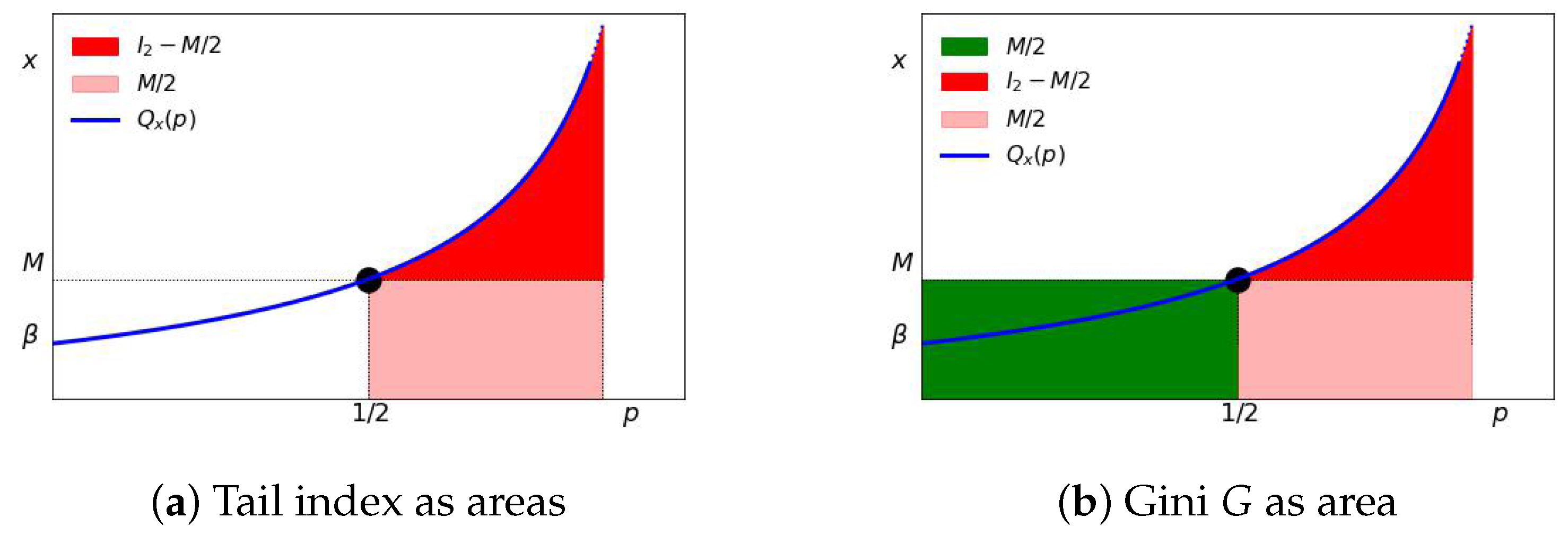
If we re-write this as $H=(I_2-M/2)+(M/2-I_1)$, then H has a simple geometrical interpretation as the shaded area shown in Figure 3b.

Unlike the standard deviation, which is based on the $L_2$-norm, the mean absolute deviation is an $L_1$-metric and offers a direct and more explainable metric of deviations Dodge (1987); K. Elsayed (2015); Pham-Gia and Hung (2001); Rousseeuw and Croux (1993). When applied to the Pareto distribution, the mean absolute deviation H also has a simple “economic” interpretation. We can interpret $I_1$ as one-half of the average income of the (0–50%) lower-half income households, whereas $I_2$ is one-half of the average income of the (50–100%) income households. The mean absolute deviation from the median H in Equation (14) can therefore be interpreted as one-half of the difference in mean incomes between the upper- and lower-half income groups.

Finally, let us now relate the mean absolute deviation to skewness. Consider the Groeneveld and Meeden’s skewness Groeneveld and Meeden (1984) coefficient S is defined as

$$S={\displaystyle \frac{\mu -M}{H}}$$

(15)

In economic terms, the numerator $(\mu -M)$ is the difference between the mean income $\mu$ and the median income M. The denominator $H=(I_2-I_1)$ is one-half of the difference between the average income of the upper half (50–100%) income bracket and the lower half (0–50%) income bracket.

5. Interpreting the Tail and the Gini Index

One of the metrics for this distribution is the Gini index G that measures the deviation from equitable distribution. Formally, it is defined in terms of the so-called Lorenz curve $L\left(p\right)$

$$L\left(x\right)={\displaystyle \frac{{\displaystyle {\int }_{\beta }^{x}tf\left(t\right)dt}}{{\displaystyle {\int }_{\beta }^{\infty }tf\left(t\right)dt}}}$$

(16)

The Lorenz curve shows the percentage of income earned by people below the value x. For the Pareto distribution, the Lorenz curve $L\left(p\right)$ and the Gini index G are

$$L\left(p\right)=1-{(1-p)}^{1-1/\alpha }\mathrm{and}G={\int }_0^{1}L\left(p\right)dp={\displaystyle \frac{1}{2\alpha -1}}$$

(17)

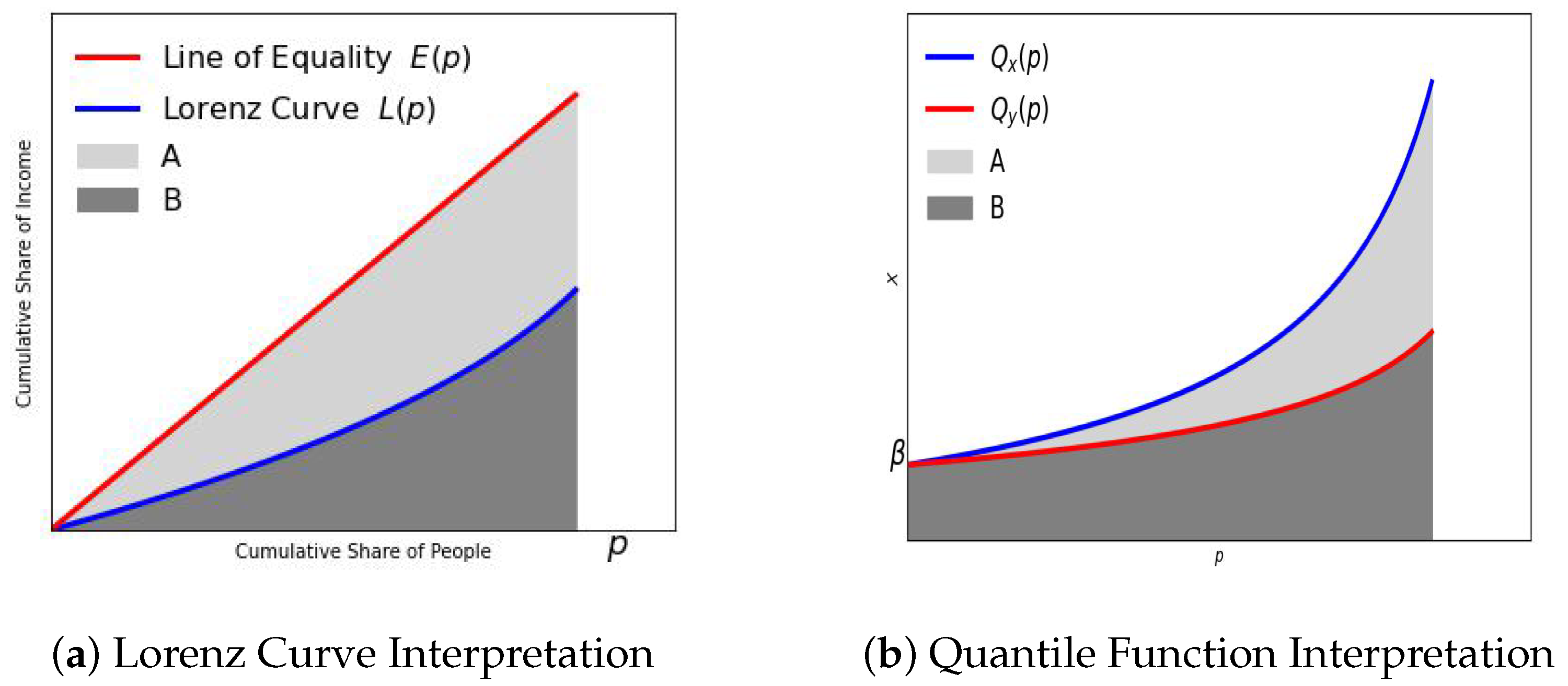
This index can be computed as the ratio of area $A/(A+B)$ under the Lorenz curve. This is illustrated in Figure 4a.

The coefficient G tells us how far the Lorenz curve $L\left(x\right)$ is from the line of equality $E\left(p\right)$. The Gini coefficient G is equal to the area $(A+B)$ below the line of perfect equality $E\left(p\right)$ minus the area B below the Lorenz curve $L\left(p\right)$, divided by the area $(A+B)$ below the line of perfect equality $E\left(p\right)$. In other words, $G=A/(A+B)$.

We can derive a similar interpretation in terms of the quantile functions. Consider two random variables, X and Y, both with the same $\beta$ but with tail indices $\alpha$ and $2\alpha$ respectively. As before, we assume $\alpha >1$. Note that a larger $\alpha$ represents a more equitable distribution.

Let $Q_x\left(p\right)$ and $Q_y\left(p\right)$ denote their corresponding quantile functions. The means ${\mu }_x$ and ${\mu }_y$ can be computed as areas under their quartile functions:

$${\mu }_x={\int }_0^1{Q}_x\left(p\right)dp\mathrm{and}{\mu }_y={\int }_0^1{Q}_y\left(p\right)dp$$

(18)

On the other hand, for Pareto distributions with $\alpha >1$, these means are ${\mu }_x=\alpha \beta /(\alpha -1)$ and ${\mu }_y=2\alpha \beta /(2\alpha -1)$ respectively. Then

$${\mu }_y-{\mu }_x={\displaystyle \frac{\alpha \beta }{(\alpha -1)}}\left({\displaystyle \frac{1}{2\alpha -1}}\right)={\mu }_x{G}_x⟹G_x={\displaystyle \frac{{\mu }_y-{\mu }_x}{{\mu }_x}}$$

(19)

If the means ${\mu }_x$ and ${\mu }_y$ represent the areas $(A+B)$ and B under the corresponding quantile functions, we can interpret the Gini coefficient as follows: The Gini coefficient G is equal to the area $(A+B)$ below the quantile function of X minus the area B below the quantile function of Y divided by the area $(A+B)$ below the quantile function of X. In other words, $G=A/(A+B)$. This is illustrated in Figure 4b. This explanation is analogous to the explanation of G in terms of the Lorenz curve shown in Figure 4a.

Finally, throughout this paper, we will use the following: for any two constants A and B such that

$${\displaystyle \frac{\alpha }{(\alpha -1)}}A=B$$

(20)

we have

$$\alpha =1+{\displaystyle \frac{A}{B-A}}\mathrm{and}G=1-{\displaystyle \frac{2A}{B+A}}$$

(21)

For example, if we apply this to the formula for the mean of the Pareto distribution with $A=\beta$ and $B=\mu$, then we obtain

$$\alpha =1+{\displaystyle \frac{\beta }{\mu -\beta }}\mathrm{and}G=1-{\displaystyle \frac{2\beta }{\mu +\beta }}$$

(22)

This has the following geometric explanation in terms of the quantile function shown in Figure 5.

In the case of perfect inequality (one person has all the wealth), the tail index $\alpha =1$ and the Gini coefficient is 1. The term $\beta /(\mu -\beta )$ in the expression for $\alpha$ and the term $2\beta /(\mu +\beta )$ in Equation (22) measure deviation from such a perfect inequality. On the other extreme, in the case of perfect equality (everyone has the same income $\beta$), the tail index $\alpha$ is infinite and the Gini coefficient $G=0$. In such a case, all income would be equal, and the mean income $\mu$ would be the same as the minimum income $\beta$. Therefore, the function $y\left(p\right)=\beta$ represents the quantile function of “total equality” with the area under $y\left(p\right)$ for $0\le p\le 1$ equal to $\beta$. The mean $\mu$ for the Pareto distribution is the area under the quantile curve shown in Figure 5a. The term $(\mu -\beta )$ is the average minus the minimum income $\beta$ and represents deviation from the equality case. Therefore, the term $\beta /(\mu -\beta )$ in Equation (22) represents deviation from perfect inequality for $\alpha$, whereas the term $2\beta /(\mu +\beta )$ represents the deviation of the Gini coefficient from the perfect inequality. This is shown in Figure 5b.

This interpretation of $\alpha$ and G in terms of the ratio of areas under the quantile function in Figure 5b in Equation (22) is analogous to the interpretation of G in terms of the ratios of areas under the Lorenz curve in Figure 4b in Equation (17).

Interpretation of the Tail Index and Gini Coefficient in Terms of Mean Absolute Deviation

Alternatively, we can interpret $\alpha$ and G in terms of the mean absolute deviations. First, we provide a geometric interpretation for $\alpha$.

For the Pareto distribution, from Equation (12) we have

$$\begin{array}{cc}\hfill I_1& ={\int }_{{\displaystyle \raisebox{1ex}{$1$}\!\left/ \!\raisebox{-1ex}{$2$}\right.}}^{1}Q\left(p\right)dp=\left({\displaystyle \frac{\alpha }{\alpha -1}}\right)\left(\beta -{\displaystyle \frac{M}{2}}\right)\hfill \\ \hfill I_2& ={\int }_0^{{\displaystyle \raisebox{1ex}{$1$}\!\left/ \!\raisebox{-1ex}{$2$}\right.}}Q\left(p\right)dp=\left({\displaystyle \frac{\alpha }{\alpha -1}}\right){\displaystyle \frac{M}{2}}\hfill \end{array}$$

(23)

Since for the Pareto distribution with $\alpha >1$, the mean $\mu$ is finite and $\mu =\alpha \beta /(\alpha -1)$, we can easily evaluate H from Equation (14) as follows:

$$H=I_2-I_1=\mu -\left({\displaystyle \frac{\alpha }{\alpha -1}}\right)M$$

(24)

After some simple algebra, we obtain

$$\alpha ={\displaystyle \frac{H+\mu }{H+\mu -M}}={\displaystyle \frac{I_2}{I_2-M/2}}\mathrm{and}G={\displaystyle \frac{H+\mu -M}{H+\mu +M}}={\displaystyle \frac{I_2-M/2}{I_2+M/2}}$$

(25)

This is illustrated in Figure 6.

Finally, let us relate the mean absolute deviation H, the mean $\mu$, and the Lorenz curve. Since $L(1/2)=1-2^{1/\alpha -1}$, we have

$$I_1={\displaystyle \frac{\alpha \beta }{(\alpha -1)}}L\left({\displaystyle \raisebox{1ex}{$1$}\!\left/ \!\raisebox{-1ex}{$2$}\right.}\right),\mathrm{and}{I}_2={\displaystyle \frac{\alpha \beta }{(\alpha -1)}}\left(1-L\left({\displaystyle \raisebox{1ex}{$1$}\!\left/ \!\raisebox{-1ex}{$2$}\right.}\right)\right)$$

(26)

This gives us

$$H={\displaystyle \frac{\alpha \beta }{\alpha -1}}=\mu \left(1-2L\left({\displaystyle \raisebox{1ex}{$1$}\!\left/ \!\raisebox{-1ex}{$2$}\right.}\right)\right)$$

(27)

6. “Economic” Interpretation of Tail Index, Gini Index, and MAD

Let us interpret our results in economic terms. If the distribution of income X follows a Pareto distribution, then we can define any subgroup with income in the range $x_1\le X\le x_2$ and compute the average income in this group by considering the corresponding truncated distribution of X as follows. For any two values, $x_1<x_2$ let $p_1=F\left(x_1\right)$ and $p_2=F\left(x_2\right)$. Let $\mathrm{E}(x_1\le X\le x_2)$ denote the corresponding average income for that group. Then, using the truncation, we have

$$\begin{array}{cc}\hfill E(x_1\le X\le x_2)& ={\displaystyle \frac{1}{F\left(x_2\right)-F\left(x_1\right)}}{\int }_{x_1}^{x_2}xf\left(x\right)dx={\displaystyle \frac{1}{(p_2-p_1)}}{\int }_{p_1}^{p_2}Q\left(p\right)dp\hfill \\ \hfill & ={\displaystyle \frac{1}{(p_2-p_1)}}·{\displaystyle \frac{\alpha }{(\alpha -1)}}\left[(1-p_1)Q\left(p_1\right)-(1-p_2)Q\left(p_2\right)\right]\hfill \end{array}$$

(28)

For example, if we define a low-income group as households with income $\beta \le X\le Q_1$, then we have $p_1=0$ and $p_2=1/4$. From Equation (28) we obtain

$$E(\beta \le X\le Q_1)={\displaystyle \frac{4\alpha }{(\alpha -1)}}\left(\beta -{\displaystyle \frac{3}{4}}{Q}_1\right)={\displaystyle \frac{\alpha }{(\alpha -1)}}(4\beta -3Q_1)$$

(29)

In the same manner, we can define other income groups and explicitly compute their average income in terms of $\alpha$ and quartiles. This is summarized in

Table 1. Interpretation of incomes via quartiles.

Income Group	X	p	Average
0–100%	$X\ge \beta$	$0\le p\le 1$	${\displaystyle \frac{\alpha }{\alpha -1}·\beta }$
0–25%	$\beta \le X\le Q_1$	$0\le p<1/4$	${\displaystyle \frac{\alpha }{\alpha -1}·(4\beta -3Q_1)}$
25–50%	$Q_1\le X\le M$	$1/4\le p\le 1/2$	${\displaystyle \frac{\alpha }{\alpha -1}·(3Q_1-2M)}$
50–75%	$M\le X\le Q_3$	$1/2\le p\le 3/4$	${\displaystyle \frac{\alpha }{\alpha -1}·(2M-Q_3)}$
25–100%	$X\ge Q_3$	$3/4\le p\le 1$	${\displaystyle \frac{\alpha }{\alpha -1}·(4\beta -Q_3)}$
0–50%	$\beta \le X\le M$	$0\le p\le 1/2$	${\displaystyle \frac{\alpha }{\alpha -1}·(2\beta -M)}$
50–100%	$X\ge M$	$1/2\le p\le 1$	${\displaystyle \frac{\alpha }{\alpha -1}·M}$
25–75%	$Q_1\le X\le Q_3$	$1/4\le p\le 3/4$	${\displaystyle \frac{\alpha }{\alpha -1}·\left(\frac{3Q_1-Q_3}{2}\right)}$
0–75%	$\beta \le X\le Q_3$	$0\le p\le 3/4$	${\displaystyle \frac{\alpha }{\alpha -1}·\left(\frac{4\beta -Q_3}{3}\right)}$
75–100%	$X\ge Q_1$	$1/4\le p\le 1$	${\displaystyle \frac{\alpha }{\alpha -1}·\left(\frac{4\beta +3Q_1}{3}\right)}$

.

From this table, we can interpret $I_1$ as one-half of the average income of the (25–50%) lower-half income households, whereas $I_2$ is one-half of the average income of the (50–75%) income households. The mean absolute deviation from the median H in Equation (14) can be interpreted as one-half of the difference in mean incomes between the upper- and lower-half income groups.

The tail index $\alpha$ in Equation (25) can be written as $\alpha =2I_2/(2I_2-M)$. This gives us the following simple interpretation: The tail index is the ratio of the average income $2I_2$ of the (50–75%) income group divided by the differences between this average and the median income, namely $(2I_2-M)$.

The Gini index $\alpha$ in Equation (25) can be written as $G=(2I_2-M)/(2I_2+M)$. This gives us the following simple interpretation: The Gini index is the ratio of the difference between the average income and the median $(2I_2-M)$ of the (50–75%) income divided by the sum of this average and the median income, namely $(2I_2+M)$.

Finally, we note that for the Pareto distribution, for any average income above some $x=Q\left(p\right)$, we have

$$\mathrm{E}(X\ge x)={\displaystyle \frac{\alpha }{(\alpha -1)}}Q\left(p\right)$$

(30)

Therefore, the ratio of the average income above any threshold $X=x$ to the corresponding rank $Q\left(p\right)$ is independent of x and is just $b=\alpha /(\alpha -1)$. The term b is referred to as the inverted Pareto coefficient. It represents a measure of income at the top of the distribution and describes the tail of the distribution. In this paper, we will continue to express our formulas in terms of the tail index $\alpha$.

7. Truncated Pareto Distribution

If X does not have a finite first moment (case $\alpha \le 1$), then at least one of the integrals on the right-hand side of Equation (6) does not converge. Moreover, in practice, we often have extreme values (“outliers”) that could have a significant effect on the results. The mean absolute deviation is not as sensitive to outliers as the standard deviation, especially if one uses mean absolute deviation around the median (as we do) and not around the mean Leys et al. (2013).

Many models in statistical analysis assume finite mean or variance. Many models with a Pareto distribution assume a finite mean ($\alpha >1$). However, there are many models for datasets with heavy tails for which the finite moment does not exist. Such models are used to describe catastrophic losses in risk management.

To address this, we can consider a truncated random variable $X^{\ast }$ restricted to $Q_1\le x\le Q_3$. When applied to real datasets, truncation allows the removal of extreme values in the distribution. For this truncated distribution, its density $f^{\ast }\left(x\right)$ and its cumulative distribution $F^{\ast }\left(x\right)$ are Papoulis (1984)

$$f^{\ast }\left(x\right)=2f\left(x\right),F^{\ast }\left(x\right)=2F\left(x\right)-1/2,x\in (Q_1,Q_3)$$

(31)

The median of the truncated random variable $X^{\ast }$ is $M^{\ast }=M\left(F\left(Q_1\right)+F\left(Q_3\right)\right)=M$ and coincides with the median M of the original distribution X.

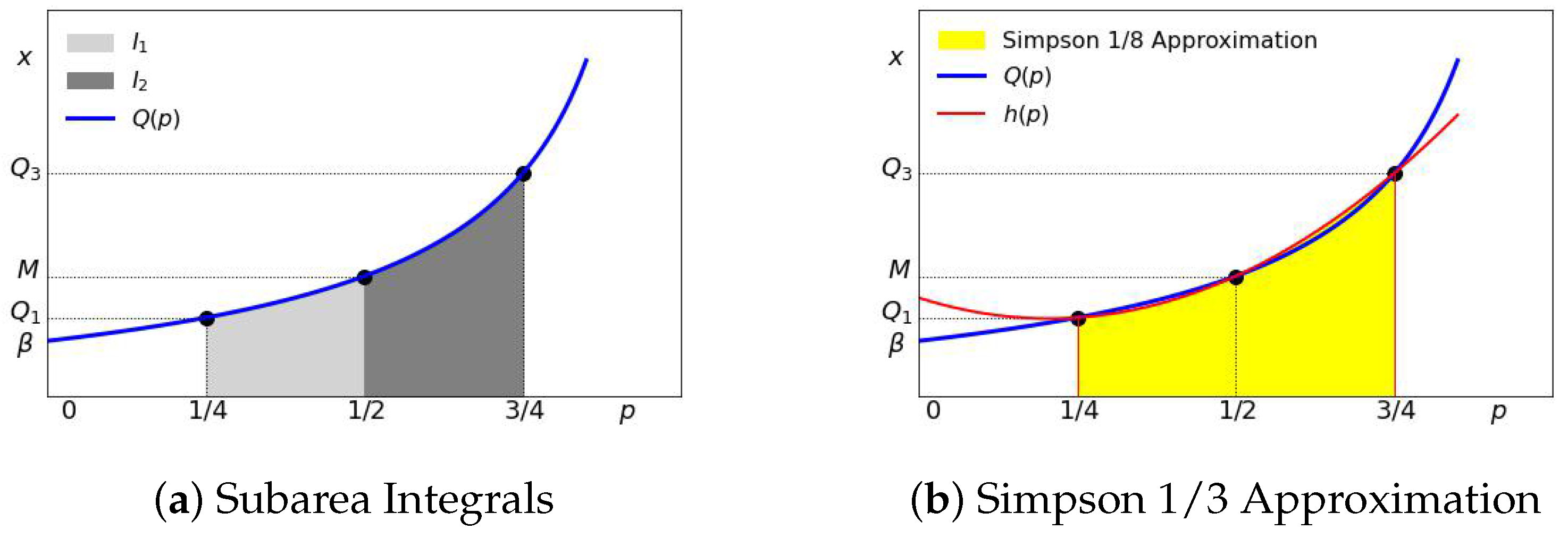
We now address the issue of computing the mean absolute deviation $H^{\ast }\left(M\right)$ of a truncated random variable $X^{\ast }$ around its median M using the original quantile function $Q\left(p\right)$ for X. To that end, we will find it convenient to introduce the following two “subarea” integrals:

$$I_1^{\ast }={\int }_{{\displaystyle \raisebox{1ex}{$1$}\!\left/ \!\raisebox{-1ex}{$4$}\right.}}^{{\displaystyle \raisebox{1ex}{$1$}\!\left/ \!\raisebox{-1ex}{$2$}\right.}}Q\left(p\right)dp\mathrm{and}{I}_2^{\ast }={\int }_{{\displaystyle \raisebox{1ex}{$1$}\!\left/ \!\raisebox{-1ex}{$2$}\right.}}^{{\displaystyle \raisebox{1ex}{$3$}\!\left/ \!\raisebox{-1ex}{$4$}\right.}}Q\left(p\right)dp$$

(32)

Then, we can write the equation for the mean absolute deviation $H^{\ast }$ of the truncated distribution $H^{\ast }$ around its median $M=Q_2$ as follows:

$$\begin{array}{cc}\hfill H^{\ast }& ={\int }_{Q_1}^{Q_3}|x-M|f^{\ast }\left(x\right)dx=2{\int }_{Q_1}^M(M-x)f\left(x\right)dx+2{\int }_M^{Q_3}(x-M)f\left(x\right)dx\hfill \\ \hfill & =2\left[M{\int }_{Q_1}^{M}f\left(x\right)dx-{\int }_{Q_1}^{M}xf\left(x\right)dx\right]+2\left[{\int }_M^{Q_3}xf\left(x\right)dx-M{\int }_M^{Q_3}f\left(x\right)dx\right]\hfill \\ \hfill & =2\left[{\displaystyle \frac{M}{4}}-{\int }_{{\displaystyle \raisebox{1ex}{$1$}\!\left/ \!\raisebox{-1ex}{$4$}\right.}}^{{\displaystyle \raisebox{1ex}{$1$}\!\left/ \!\raisebox{-1ex}{$2$}\right.}}Q\left(p\right)dp\right]+2\left[{\int }_{{\displaystyle \raisebox{1ex}{$1$}\!\left/ \!\raisebox{-1ex}{$2$}\right.}}^{{\displaystyle \raisebox{1ex}{$3$}\!\left/ \!\raisebox{-1ex}{$4$}\right.}}Q\left(p\right)dp-{\displaystyle \frac{M}{4}}\right]=2(I_2^{\ast }-I_1^{\ast })\hfill \end{array}$$

(33)

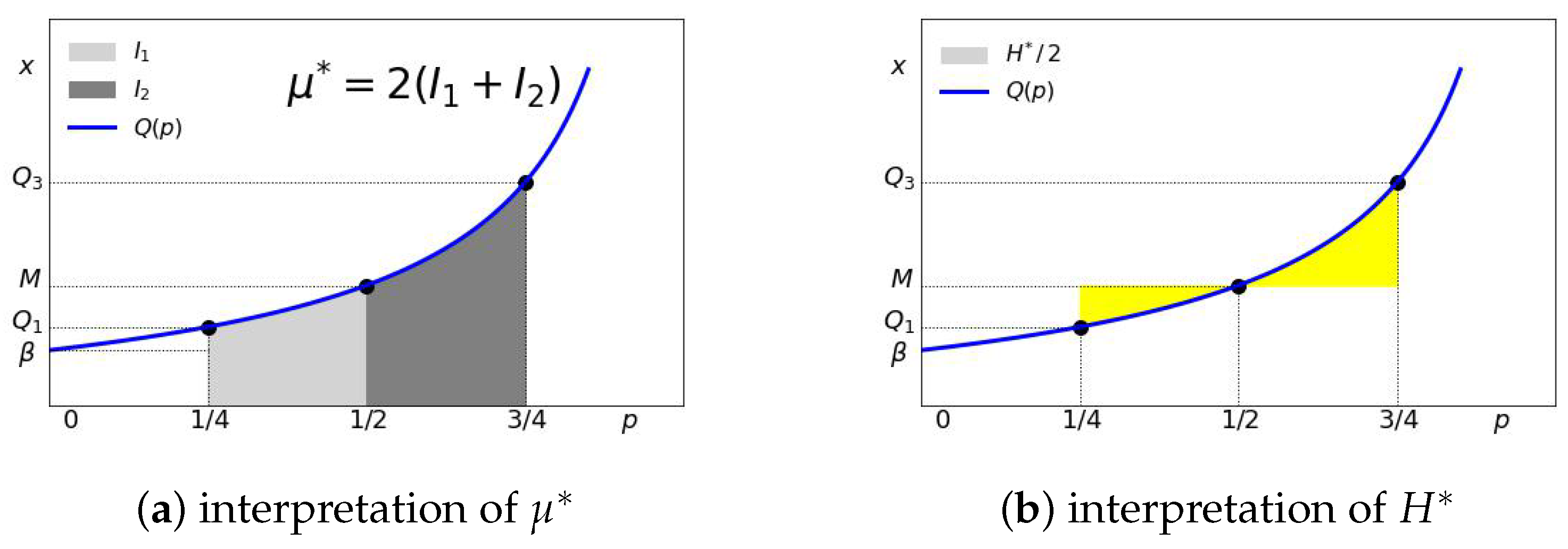
The mean absolute deviation $H^{\ast }$ of the truncated variable $X^{\ast }$ around the median M is twice the difference between the right and left sub-means. Note that the mean ${\mu }^{\ast }$ of the truncated distribution

$${\mu }^{\ast }={\int }_{Q_1}^{Q_3}x{f}^{\ast }\left(x\right)dx=2{\int }_{{\displaystyle \raisebox{1ex}{$1$}\!\left/ \!\raisebox{-1ex}{$4$}\right.}}^{{\displaystyle \raisebox{1ex}{$3$}\!\left/ \!\raisebox{-1ex}{$4$}\right.}}Q\left(p\right)dp=2(I_1^{\ast }+I_2^{\ast })$$

(34)

The subareas $I_1^{\ast }$ and $I_2^{\ast }$ correspond to left and right sub-means for $X^{\ast }$ between $p=1/4$ and $p1/2$ and between $1/2$ and $3/4$, respectively. This is illustrated in Figure 7.

The subarea $I_1^{\ast }$ represents the average income in the $25=50\%$ income group, whereas the subarea $I_2$ represents the average income in the 50–75% income group. It is interesting to compare the above expression for the mean absolute deviation of $H^{\ast }=2(I_2^{\ast }-I_1^{\ast })$ of the truncated random variable $X^{\ast }$ in Equation (34) with the equation for the mean absolute deviation $H=(I_2-I_1)$ of X in Equation (24). As we discussed in Section 6, the mean absolute deviation H can be interpreted as a difference in average incomes of the top (50–100%) and bottom (50–100%) income groups. By contrast, the mean absolute deviation $H^{\ast }$ can be interpreted as twice the difference in average incomes of the top (50–75%) and bottom (25–50%) income groups in the truncated distribution.

We now compute the subareas $I_1^{\ast }$ and $I_2^{\ast }$ explicitly. For the left sub-area $I_1^{\ast }$, from Equation (12), we have

$$I_1^{\ast }={\int }_{{\displaystyle \raisebox{1ex}{$1$}\!\left/ \!\raisebox{-1ex}{$4$}\right.}}^{{\displaystyle \raisebox{1ex}{$1$}\!\left/ \!\raisebox{-1ex}{$2$}\right.}}Q\left(p\right)dp={\displaystyle \frac{\alpha }{\alpha -1}}\left({\displaystyle \frac{3}{4}}{Q}_1-{\displaystyle \frac{1}{2}}M\right)$$

(35)

Similarly, for the right sub-area $I_2^{\ast }$ from Equation (12), we have

$$I_2^{\ast }={\int }_{{\displaystyle \raisebox{1ex}{$1$}\!\left/ \!\raisebox{-1ex}{$2$}\right.}}^{{\displaystyle \raisebox{1ex}{$3$}\!\left/ \!\raisebox{-1ex}{$4$}\right.}}Q\left(p\right)dp={\displaystyle \frac{\alpha }{\alpha -1}}\left({\displaystyle \frac{1}{2}}M-{\displaystyle \frac{1}{4}}{Q}_3\right)$$

(36)

For the mean absolute deviation $H^{\ast }=2(I_2^{\ast }-I_1^{\ast })$, we obtain

$$H^{\ast }={\displaystyle \frac{\alpha }{\alpha -1}}\left[2M-\left({\displaystyle \frac{3}{2}}{Q}_1+{\displaystyle \frac{1}{2}}{Q}_3\right)\right]$$

(37)

whereas for mean ${\mu }^{\ast }=2(I_1^{\ast }+I_2^{\ast })$ we obtain

$$\begin{array}{|c|}\hline {\mu }^{\ast }={\displaystyle \frac{\alpha }{\alpha -1}}·\left({\displaystyle \frac{3}{2}}{Q}_1-{\displaystyle \frac{1}{2}}{Q}_3\right)\\ \hline\end{array}$$

(38)

We will use the above result in Equation (38) and consider different approximations to subarea integrals. The problem of estimating such integrals is called numerical integration or numerical quadrature and is a classical and well-researched problem in numerical analysis Conte and De Boor (1972). This problem arises when the integration cannot be carried out or when the function is known only at a finite number of points.

When applied to estimating the subarea integrals with numerical quadrature, these integrals are approximated at points $p={\displaystyle \raisebox{1ex}{$1$}\!\left/ \!\raisebox{-1ex}{$/$}\right.}4$, $p={\displaystyle \raisebox{1ex}{$1$}\!\left/ \!\raisebox{-1ex}{$2$}\right.}$, and $p={\displaystyle \raisebox{1ex}{$3$}\!\left/ \!\raisebox{-1ex}{$4$}\right.}$. This would allow us to derive explicit closed-form approximations for $\alpha$ and G in terms of quartiles. This would be addressed in Section 9.

We can rewrite this in terms of the Lorenz curve. From Equations (3) and (17) we have:

$$L\left({\displaystyle \raisebox{1ex}{$1$}\!\left/ \!\raisebox{-1ex}{$4$}\right.}\right)=1-{(4/3)}^{1/\alpha -1},L\left({\displaystyle \raisebox{1ex}{$1$}\!\left/ \!\raisebox{-1ex}{$2$}\right.}\right)=1-{(1/2)}^{1/\alpha -1},L\left({\displaystyle \raisebox{1ex}{$3$}\!\left/ \!\raisebox{-1ex}{$4$}\right.}\right)=1-4^{1/\alpha -1}$$

(39)

and therefore, we can rewrite Equations (35) and (36) for subarea integrals $I_1^{\ast }$ and $I_2^{\ast }$ as:

$$I_1^{\ast }={\displaystyle \frac{\alpha \beta }{(\alpha -1)}}\left[L\left({\displaystyle \raisebox{1ex}{$1$}\!\left/ \!\raisebox{-1ex}{$2$}\right.}\right)-L\left({\displaystyle \raisebox{1ex}{$1$}\!\left/ \!\raisebox{-1ex}{$4$}\right.}\right)\right]\mathrm{and}{I}_2^{\ast }={\displaystyle \frac{\alpha \beta }{(\alpha -1)}}\left[L\left({\displaystyle \raisebox{1ex}{$3$}\!\left/ \!\raisebox{-1ex}{$4$}\right.}\right)-L\left({\displaystyle \raisebox{1ex}{$1$}\!\left/ \!\raisebox{-1ex}{$2$}\right.}\right)\right]$$

(40)

This immediately gives us

$$H^{\ast }={\displaystyle \frac{2\alpha \beta }{(\alpha -1)}}\left[2L\left({\displaystyle \raisebox{1ex}{$1$}\!\left/ \!\raisebox{-1ex}{$2$}\right.}\right)-L\left({\displaystyle \raisebox{1ex}{$1$}\!\left/ \!\raisebox{-1ex}{$4$}\right.}\right)-L\left({\displaystyle \raisebox{1ex}{$3$}\!\left/ \!\raisebox{-1ex}{$4$}\right.}\right)\right],{\mu }^{\ast }={\displaystyle \frac{2\alpha \beta }{(\alpha -1)}}\left[L\left({\displaystyle \raisebox{1ex}{$3$}\!\left/ \!\raisebox{-1ex}{$4$}\right.}\right)-L\left({\displaystyle \raisebox{1ex}{$1$}\!\left/ \!\raisebox{-1ex}{$4$}\right.}\right)\right]$$

(41)

Note that the expression for the mean ${\mu }^{\ast }$ in the above Equation (41) can be written in terms of the mean $\mu$ of the original distribution as

$${\mu }^{\ast }=2\mu \left[L\left({\displaystyle \raisebox{1ex}{$3$}\!\left/ \!\raisebox{-1ex}{$4$}\right.}\right)-L\left({\displaystyle \raisebox{1ex}{$1$}\!\left/ \!\raisebox{-1ex}{$4$}\right.}\right)\right]$$

(42)

For income distributions that follow the Pareto distribution, $\mu$ represents the average income of all individuals, whereas ${\mu }^{\ast }$ represents the average income of individuals with income in the range $(Q_1,Q_3)$. The term in brackets represents the fraction of total wealth held by such individuals. For $\alpha \mapsto 1$ (equal distribution), we have

$${\mu }^{\ast }=2\mu \left[\left(1-{\displaystyle \frac{1}{4}}{\left({\displaystyle \frac{1}{4}}\right)}^{1/\alpha }\right)-\left(1-{\displaystyle \frac{3}{4}}{\left({\displaystyle \frac{4}{3}}\right)}^{1/\alpha }\right)\right]\mapsto \mu /2$$

(43)

as expected.

We can provide a quantile interpretation of income inequality. The average income in the (25–75%) income bracket is ${\mu }^{\ast }$, shown in Figure 8a. If everyone had the same (minimum) income $\beta$, then we would have ${\mu }^{\ast }=\beta$. The difference $({\mu }^{\ast }-\beta )$ between the average (truncated) income ${\mu }^{\ast }$ and the minimum income $\beta$ represents the deviation from the equality. This is illustrated in Figure 8b.

This is analogous to the interpretation of inequality in terms of the overall mean $\mu$ and $\beta$ shown in Figure 6.

The approach outlined above of truncating the distribution at the quartiles and estimating the parameters by computing the subarea integrals of the quantile functions between ${\displaystyle \raisebox{1ex}{$1$}\!\left/ \!\raisebox{-1ex}{$4$}\right.}$ and ${\displaystyle \raisebox{1ex}{$3$}\!\left/ \!\raisebox{-1ex}{$4$}\right.}$ is quite general. It can be applied to distributions with or without finite moments or variances if the quantile function is available. Such distributions arise in many areas of risk management and finance Chen and Wang (2025).

We can consider such an approach and obtain closed-form approximations for parameters for a number of important distributions, including the Levy distribution, which does not have any moments, and the Gumbel extreme-value distribution. These distributions are widely used in risk management and finance Rachev (2003).

In particular, for the Levy distribution, the quantile function can be expressed in terms of the inverse of the Gaussian CDF $\Phi (·)$ and is

$$Q\left(p\right)=\mu +{\displaystyle \frac{c}{{\left[{\Phi }^{-1}(1-p/2)\right]}^2}}$$

(44)

and using the approach outlined above, we were able to derive simple approximations for the parameters by truncating the distribution at the quartiles and expressing the subarea integrals in terms of the corresponding quartiles and octiles of the normal distribution.

For the Gumbel distribution with location $\mu$ and scale $\beta$, the quantile function is

$$Q\left(p\right)=\mu -\beta log(-log(p\left)\right)$$

(45)

Using our approach, we should be able to compute the parameters in terms of quartiles and logarithmic integrals (constants).

When applied to Pareto, one immediate extension is the Generalized Pareto IV distribution with the quantile function

$$Q\left(p\right)=\mu +{\displaystyle \frac{\sigma }{\xi }}\left[{(1-p)}^{-\xi }-1\right]$$

(46)

This includes Pareto distribution ($\xi >0$ and $\mu =\sigma /\xi$), exponential ($\xi =\mu =0$), Lomax distribution ($\mu =0$), and many others. When applied to financial markets, this distribution can be used to model extreme events and estimate the Value at Risk (VaR) and the expected shortfall (ES). Our method would allow a simple estimation of these quantities via the quartiles. This would allow us to see the effect of the upper-tail behavior on volatility and returns.

Unlike the Pareto distribution considered in this paper, the generalized Pareto distribution has multiple parameters. To estimate these, we can consider an MAD-based approach: As before, we consider a truncated distribution, but we estimate three mean absolute deviations, $H\left(Q_1\right)$, $H\left(M\right)$, $H\left(Q_3\right)$, around the quartiles as well as the truncated mean ${\mu }^{\ast }$. This gives us four equations in four unknowns that can be solved numerically. For many other distributions, such as log-normal, Cauchy, and Weibull, we can derive closed-form solutions for the parameters in terms of simple formulas involving the quartiles. We hope to address the analysis of the generalized Pareto distribution in our future work.

8. Approximating Tail and Gini Index Using the Mean Absolute Deviation of the Truncated Distribution

In this section, we derive approximations to the tail index and Gini index using the mean absolute deviation $H^{\ast }$ of the truncated distribution. We will call this method $H^{\ast }$-based. We proceed as follows. From Equation (37), we obtain

$$\alpha ={\displaystyle \frac{H^{\ast }}{H^{\ast }-\left(M-(3Q_1+Q_3)/2\right)}},G={\displaystyle \frac{H^{\ast }-\left(M-(3Q_1+Q_3)/2\right)}{H^{\ast }+\left(M-(3Q_1+Q_3)/2\right)}}$$

(47)

In terms of subarea integrals, we can rewrite these expressions as

$$\alpha ={\displaystyle \frac{2(I_2^{\ast }-I_1^{\ast })}{2(I_2^{\ast }-I_1^{\ast })-\left(M-(3Q_1+Q_3)/2\right)}},G={\displaystyle \frac{2(I_2^{\ast }-I_1^{\ast })-\left(M-(3Q_1+Q_3)/2\right)}{2(I_2^{\ast }-I_1^{\ast })+\left(M-(3Q_1+Q_3)/2\right)}}$$

To compute $\alpha$ and G, we propose to approximate subarea integrals $I_1^{\ast }$ and $I_2^{\ast }$ by numeric quadrature. In quadrature approximation, we approximate the integral of a function with a weighted sum of functions, the so-called “abscissas” or “Quadrature points” Rudin (1976). When the function in question is a quantile function, its integral is approximated by a weighted sum of quantiles. To illustrate this with a very simple example, consider the integral of the quantile function between points $p_1$ and $p_2$. This integral is approximated by the area of a rectangle with base length $(p_2-p_1)$ and height $Q\left(p_1\right)$. In this paper, we will confine ourselves to very simple rules, such as the “midpoint”, trapezoid, and Simpson rules Olver et al. (2010). We will show that even these simple rules provide valuable insights into interpreting the shape metrics.

Let us consider the so-called trapezoid rule Rudin (1976): $I_1^{\ast }\approx (Q_1+M)/8$ and $I_2^{\ast }\approx (M+Q_3)/8$. From Table 1 this can be interpreted as setting the average income $\mathrm{E}(Q_1\le X\le M)$ of the (25–50%) group to $(Q_1+M)/2$ and setting the average income $\mathrm{E}(M\le X\le Q_3)$ of the (50–75%) group to $(Q_3+M)/2$. The difference of subarea integrals $(I_2^{\ast }-I_1^{\ast })$ is then $(Q_3-Q_1)/8$. This is illustrated in Figure 9.

With this approximation for $(I_2-I_1)$, we obtain

$$\begin{array}{cc}\hfill H^{\ast }& \approx {\displaystyle \frac{1}{4}}(Q_3-Q_1),\alpha \approx {\displaystyle \frac{1}{2}}\left({\displaystyle \frac{Q_3-Q_1}{Q_1+Q_3-2M}}\right),G\approx {\displaystyle \frac{1}{2}}\left({\displaystyle \frac{Q_1+Q_3-2M}{M-Q_1}}\right)\hfill \end{array}$$

(48)

These equations have a simple interpretation in terms of well-known metrics used in quantile statistics Gilchrist (2000) summarized in

Table 2. Common quantile metrics.

Name	Formula
lower quartile difference	$M-Q_1$
upper quartile difference	$Q_3-M$
quartile difference	$Q_1+Q_3-2M$
interquartile range (IQR)	$Q_3-Q_1$
Galton skewness	$(Q_1+Q_3-2M)/(Q_3-Q_1)$
skewness ratio	$(Q_3-M)/(M-Q_1)$

.

We can interpret the performance metrics in Equation (48). In terms of these metrics, obtain the following simple interpretation:

• The mean absolute deviation $H^{\ast }$ of the truncated distribution around its median is approximately a quarter of the interquartile range $(Q_3-Q_1)$;
• The tail index $\alpha$ is approximately one-half of the inverse of the Galton skewness;
• The Gini index G is one-half of the ratio of the quartile difference to the lower quartile difference $(M-Q_1)$.

We will find it convenient to consider the weighted quartile difference $R\left(w\right)$ with $0\le w\le 1$, defined as

$$R\left(w\right)=w·(M-Q_1)+(1-w)·(Q_3-M)$$

(49)

This quantile metric $R\left(w\right)$ measures the spread of data with different weights w and $(1-w)$ assigned to lower and upper quartile differences $(M-Q_1)$ and $(Q_3-M)$, respectively. With this metric, we can express our results in Equation (48) as

$$H^{\ast }\approx {\displaystyle \frac{R\left(0\right)+R\left(1\right)}{8}},\alpha \approx {\displaystyle \frac{1}{2}}\left({\displaystyle \frac{R\left(0\right)+R\left(1\right)}{R\left(0\right)-R\left(1\right)}}\right)G\approx {\displaystyle \frac{1}{2}}\left({\displaystyle \frac{R\left(0\right)}{R\left(1\right)}}-1\right)$$

(50)

9. Approximating Tail and Gini Index Using the Mean of the Truncated Distribution

In this section, we will derive approximations for $\alpha$ and G using the mean ${\mu }^{\ast }$ of the truncated distribution. In economic terms, we estimate these parameters by different approximations to the mean income. To proceed, let us define $I^{\ast }=(I_1+I_2)$ as the total subarea under $Q\left(p\right)$ with $1/4\le p\le 3/4$. Then, ${\mu }^{\ast }=2I^{\ast }$, and from Equation (38), we have

$$I^{\ast }={\displaystyle \frac{\alpha }{\alpha -1}}\left({\displaystyle \frac{3}{4}}{Q}_1-{\displaystyle \frac{1}{4}}{Q}_3\right)$$

(51)

From this, we obtain the following expressions for $\alpha$ and G:

$$\alpha ={\displaystyle \frac{{\mu }^{\ast }}{{\mu }^{\ast }-(3Q_1-Q_3)/2}}\mathrm{and}G={\displaystyle \frac{{\mu }^{\ast }-(3Q_1-Q_3)/2}{{\mu }^{\ast }+(3Q_1-Q_3)/2}}$$

(52)

We can now consider a number of approximation methods to approximate ${\mu }^{\ast }$ using integral quadrature methods to obtain simple approximations to the tail index $\alpha$ and the Gini coefficient G (For a comprehensive survey of integral quadrature methods, see Masud et al. (2024)). We will compare the relative error of the proposed approximations at the end of this section. We will consider the following methods:

• “Midpoint” method: approximate the mean ${\mu }^{\ast }$ by the median M;
• “One-Trapezoid” method: approximate the mean ${\mu }^{\ast }$ by the average of the first and third quartiles $Q_1$ and $Q_3$;
• “Two-Trapezoids” method: approximate the mean by the average of the median M with the average of the first and third quartiles $Q_1$ and $Q_3$;
• “Quartile Average” method: approximate the mean income ${\mu }^{\ast }$ by the average of the three quartiles $Q_1$, M, and $Q_3$;
• “Simpson 1/3” method: approximate the quantile function $Q\left(p\right)$ by a parabola passing through the quartiles. This will be shown to be equivalent to approximating the mean ${\mu }^{\ast }$ by the weighted average of “Two-Trapezois” and “Quartile Average” methods.

9.1. “Midpoint” Method for Approximating Tail and Gini Indices

Recall the midpoint rule for approximation of the integral of $g\left(x\right)$ between a and b:

$${\int }_a^{b}g\left(x\right)dx\approx (b-a)·g\left({\displaystyle \frac{a+b}{2}}\right)$$

(53)

This is illustrated in Figure 10.

Using this rule, we have $(I_1^{\ast }+I_2^{\ast })\approx M/2$, and from Equation (38), we have

$${\displaystyle \frac{\alpha }{\alpha -1}}\left({\displaystyle \frac{3Q_1-Q_3}{2}}\right)\approx M$$

(54)

From Table 1, we can interpret this approximation as follows: The average income $\mathrm{E}(Q_1\le X\le Q_3)$ of the middle (25–75%) income group is approximately the median income M.

From Equations (38) and (54), we obtain the following approximation for $\alpha$ and G:

$$\alpha =1+\left({\displaystyle \frac{3Q_1-Q_3}{2M-3Q_1+Q_3}}\right)\mathrm{and}G=1-2\left({\displaystyle \frac{3Q_1-Q_3}{2M+3Q_1-Q_3}}\right)$$

(55)

In terms of the weighted interquartile range defined in Equation (49) we can rewrite the above expression for $\alpha$ and G as

$$\alpha =1+{\displaystyle \frac{1}{2}}\left({\displaystyle \frac{M-R\left(\raisebox{1ex}{$1$}\!\left/ \!\raisebox{-1ex}{$2$}\right.\right)}{R\left(\raisebox{1ex}{$3$}\!\left/ \!\raisebox{-1ex}{$4$}\right.\right)}}\right)\mathrm{and}G=1-{\displaystyle \frac{M-R\left(\raisebox{1ex}{$1$}\!\left/ \!\raisebox{-1ex}{$2$}\right.\right)}{M-R\left(\raisebox{1ex}{$3$}\!\left/ \!\raisebox{-1ex}{$4$}\right.\right)}}$$

(56)

9.2. “One Trapezoid” Method for Approximating Tail and Gini Indices

Recall the trapezoid rule for approximation of the integral of $g\left(x\right)$ between a and b:

$${\int }_a^{b}g\left(x\right)dx\approx (b-a)·{\displaystyle \frac{g\left(a\right)+g\left(b\right)}{2}}$$

(57)

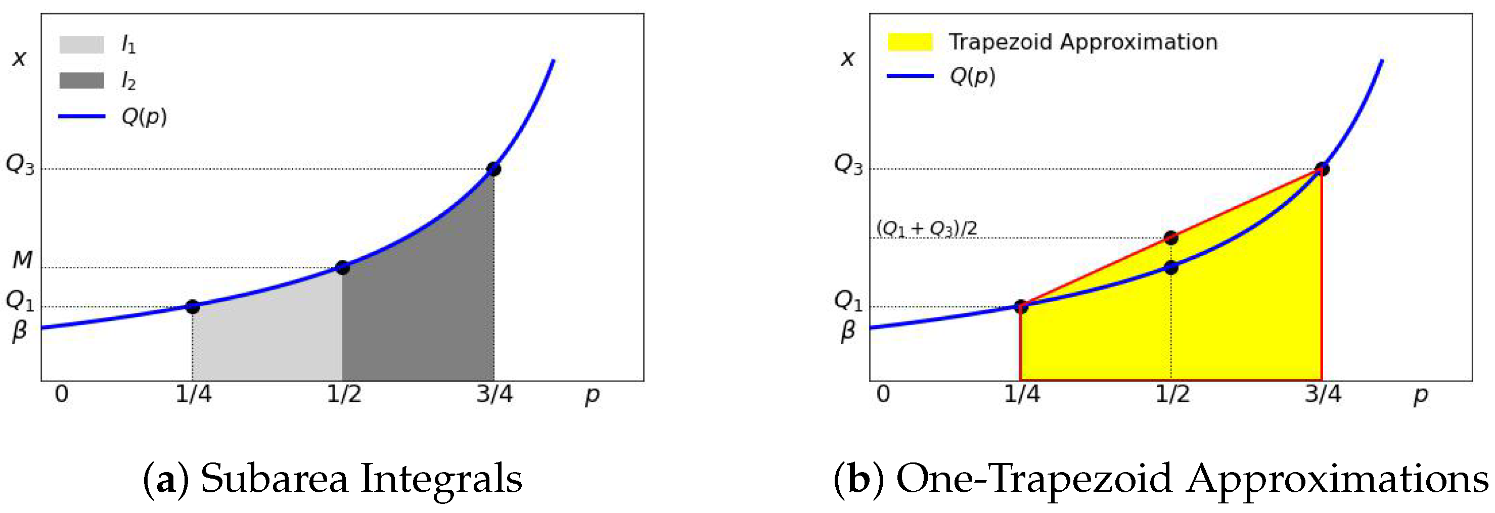
We approximate the subarea $I^{\ast }=(I_1^{\ast }+I_2^{\ast })$ by the corresponding trapezoid and obtain $I^{\ast }\approx (Q_1+Q_3)/4$. This is illustrated in Figure 11.

This can be rewritten using Equation (38) as

$${\displaystyle \frac{\alpha }{\alpha -1}}·\left({\displaystyle \frac{3Q_1-Q_3}{2}}\right)\approx {\displaystyle \frac{Q_1+Q_3}{2}}$$

(58)

From Table 1, the approximation in Equation (58) has a simple interpretation: the average income $\mathrm{E}(Q_1\le X\le Q_3)$ in the middle (25–75%) income group is approximately the average of the first and third quartiles.

From Equations (38) and (58), we get the following estimate of the tail index $\alpha$ and the Gini index G:

$$\alpha =1+{\displaystyle \frac{1}{2}}\left({\displaystyle \frac{3Q_1-Q_3}{Q_3-Q_1}}\right)\mathrm{and}G=1-{\displaystyle \frac{1}{2}}\left({\displaystyle \frac{3Q_1-Q_3}{Q_1}}\right)$$

(59)

With this approximation, the tail index $\alpha$ can be simplified to $\alpha =(Q_1+Q_3)/2(Q_3-Q_1)$. It is the average of the first and third quartiles, $Q_1$ and $Q_3$, divided by the interquartile range $\mathrm{IQR}=(Q_3-Q_1)$. The Gini coefficient can be simplified to $G=(Q_3-Q_1)/2Q_1$. The Gini coefficient G is one-half of the ratio of the interquartile range $(Q_3-Q_1)$ and the first quartile $Q_1$.

In terms of the weighted interquartile range defined in Equation (49), we can rewrite the above expression for $\alpha$ and G as

$$\alpha =1+{\displaystyle \frac{M-R\left(\raisebox{1ex}{$1$}\!\left/ \!\raisebox{-1ex}{$2$}\right.\right)}{R\left(\raisebox{1ex}{$1$}\!\left/ \!\raisebox{-1ex}{$2$}\right.\right)}}\mathrm{and}G=1-{\displaystyle \frac{M-R\left(\raisebox{1ex}{$1$}\!\left/ \!\raisebox{-1ex}{$2$}\right.\right)}{M-R\left(1\right)}}$$

(60)

9.3. “Two Trapezoids” Method for Approximating Tail and Gini Indices

If we divide the interval $[a,b]$ into n equal sub-intervals $a=x_0<x_1<\cdots <x_n=b$, then

$${\int }_a^{b}g\left(x\right)dx\approx {\displaystyle \frac{(b-a)}{n}}\sum _{i=1}^n{\displaystyle \frac{g\left(x_{i-1}\right)+g\left(x_i\right)}{2}}$$

(61)

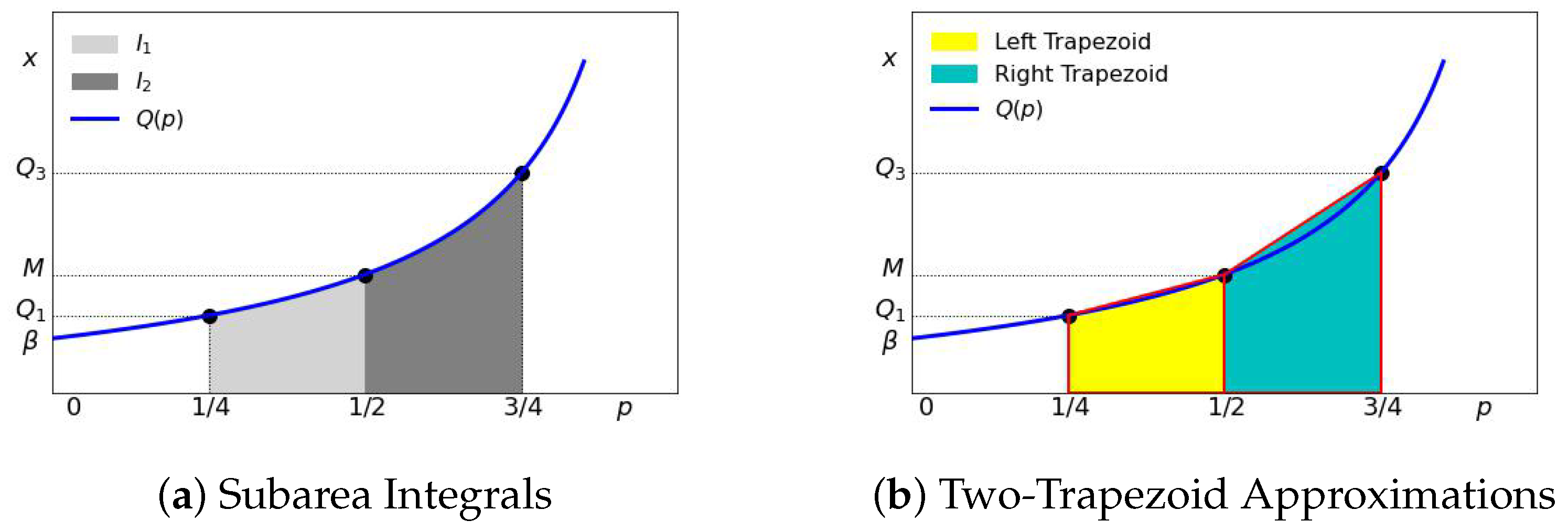
Therefore, we can consider two sub-intervals $[1/4,1/2]$ and $[1/2,3/4]$. We approximate each subareas $I_1^{\ast }$ and $I_2^{\ast }$ by separate (left and right) trapezoids: $I_1^{\ast }\approx (Q_1+M)/8$ and $I_2^{\ast }\approx (M+Q_3)/8$. This is illustrated in Figure 12.

From Table 1, this has a simple interpretation: the average income $\mathrm{E}(Q_1\le X\le M)$ in the (25–50%) income group is approximately the average of the first and second quartiles, whereas the average income $\mathrm{E}(M\le X\le Q_3)$ in the (50–75%) income group is approximately the average of the second and third quartiles.

We can rewrite this using Equation (38)

$${\displaystyle \frac{\alpha }{\alpha -1}}\left({\displaystyle \frac{3Q_1-Q_3}{2}}\right)\approx {\displaystyle \frac{Q_1+2M+Q_3}{4}}$$

(62)

From this, we get the following estimates for $\alpha$ and G:

$$\alpha =1+2\left({\displaystyle \frac{3Q_1-Q_3}{2M-5Q_1+3Q_3}}\right)\mathrm{and}G=1-4\left({\displaystyle \frac{3Q_1-Q_3}{2M+7Q_1-Q_3}}\right)$$

(63)

In terms of the weighted interquartile range defined in Equation (49), we can rewrite the above expression for $\alpha$ and G as

$$\alpha =1+{\displaystyle \frac{1}{2}}\left({\displaystyle \frac{M-R\left(\raisebox{1ex}{$1$}\!\left/ \!\raisebox{-1ex}{$2$}\right.\right)}{R\left(\raisebox{1ex}{$5$}\!\left/ \!\raisebox{-1ex}{$8$}\right.\right)}}\right)\mathrm{and}G=1-{\displaystyle \frac{M-R\left(\raisebox{1ex}{$1$}\!\left/ \!\raisebox{-1ex}{$2$}\right.\right)}{M-R\left(\raisebox{1ex}{$7$}\!\left/ \!\raisebox{-1ex}{$8$}\right.\right)}}$$

(64)

9.4. “Quartile Average” Method for Approximating Tail and Gini Indices

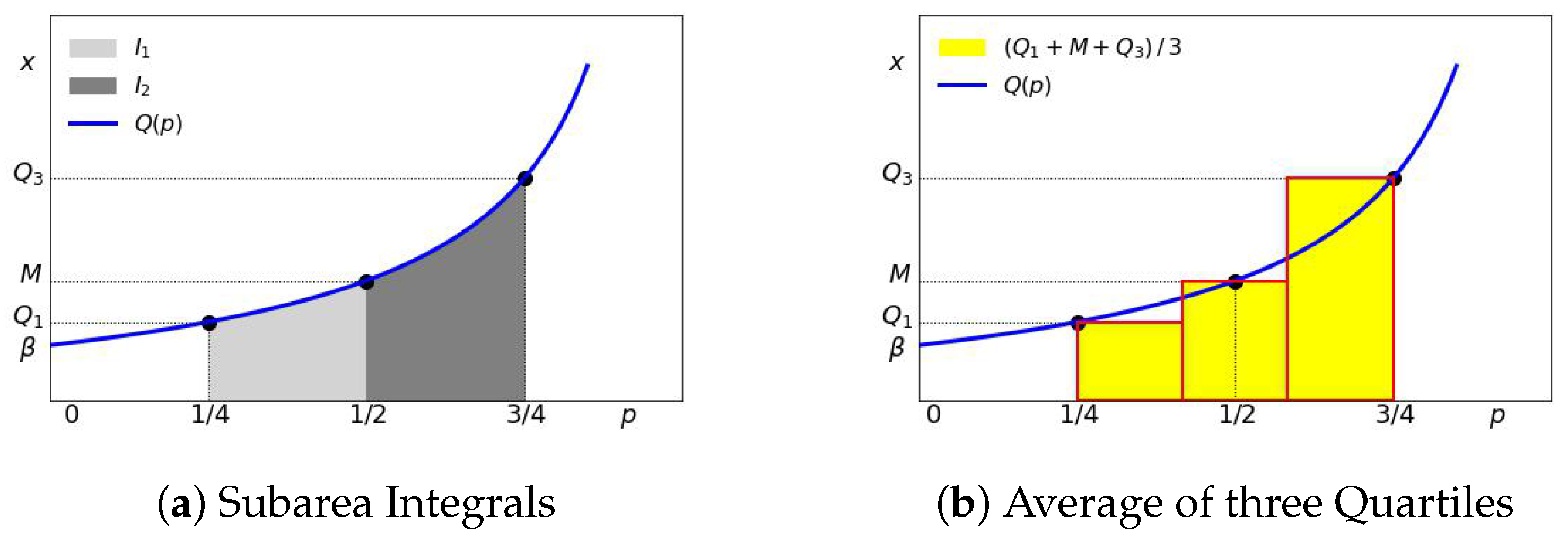
We approximate the subarea the mean value ${\mu }^{\ast }=2(I_1^{\ast }+I_2^{\ast })$ by the average $(Q_1+M+Q_3)/3$ of the three quartiles $Q_1$, M, and $Q_3$. This is illustrated in Figure 13.

From Table 1, this has a simple interpretation: the average income $\mathrm{E}(Q_1\le X\le Q_3)$ in the (25–75%) income group is approximately the average of the three quartiles $Q_1$, M, and $Q_3$.

From Equation (38), this gives us

$${\displaystyle \frac{\alpha }{\alpha -1}}\left({\displaystyle \frac{3}{2}}{Q}_1-{\displaystyle \frac{1}{2}}{Q}_3\right)={\displaystyle \frac{Q_1+M+Q_3}{3}}$$

(65)

From this, we obtain

$$\alpha =1+3\left({\displaystyle \frac{3Q_1-Q_3}{2M-7Q_1+5Q_3}}\right)\mathrm{and}G=1-6\left({\displaystyle \frac{3Q_1-Q_3}{2M+11Q_1-Q_3}}\right)$$

(66)

In terms of the weighted interquartile range defined in Equation (49) we can rewrite the above expression for $\alpha$ and G as

$$\alpha =1+{\displaystyle \frac{M-R\left(\raisebox{1ex}{$1$}\!\left/ \!\raisebox{-1ex}{$2$}\right.\right)}{R\left(\raisebox{1ex}{$7$}\!\left/ \!\raisebox{-1ex}{$12$}\right.\right)}}\mathrm{and}G=1-{\displaystyle \frac{M-R\left(\raisebox{1ex}{$1$}\!\left/ \!\raisebox{-1ex}{$2$}\right.\right)}{M-R\left(\raisebox{1ex}{$11$}\!\left/ \!\raisebox{-1ex}{$12$}\right.\right)}}$$

(67)

9.5. “Simpson 1/3” Method for Approximating Tail and Gini Indices

Recall Simpson’s rule Rudin (1976) for approximation of the integral of $g\left(x\right)$ between a and b:

$${\int }_a^{b}g\left(x\right)dx\approx {\displaystyle \frac{(b-a)}{6}}\left[g\left(a\right)+4g\left({\displaystyle \frac{a+b}{2}}\right)+g\left(b\right)\right]$$

(68)

This is accomplished by approximating the quantile function by a parabola $h\left(p\right)$ passing through the three points $({\displaystyle \raisebox{1ex}{$1$}\!\left/ \!\raisebox{-1ex}{$4$}\right.},Q_1)$, $({\displaystyle \raisebox{1ex}{$1$}\!\left/ \!\raisebox{-1ex}{$2$}\right.},M)$, and $({\displaystyle \raisebox{1ex}{$3$}\!\left/ \!\raisebox{-1ex}{$4$}\right.},Q_3)$. By the Lagrange interpolation formula Gradshteyn and Ryzhik (1980), a parabola $y\left(x\right)$ passing through three points $(x_1,y_1)$, $(x_2,y_2)$, and $(x_3,y_3)$ has the equation:

$$y\left(x\right)=y_1{\displaystyle \frac{(x-x_2)(x-x_3)}{(x_1-x_2)(x_1-x_3)}}+y_2{\displaystyle \frac{(x-x_1)(x-x_3)}{(x_2-x_1)(x_2-x_3)}}+y_3{\displaystyle \frac{(x-x_1)(x-x_2)}{(x_3-x_1)(x_3-x_2)}}$$

With this approximation, we replace the quantile function $Q\left(p\right)$ by a parabola $h\left(p\right)$:

$$\begin{array}{c}\hfill h\left(p\right)=Q_1{\displaystyle \frac{(p-\raisebox{1ex}{$1$}\!\left/ \!\raisebox{-1ex}{$2$}\right.)(p-\raisebox{1ex}{$3$}\!\left/ \!\raisebox{-1ex}{$4$}\right.)}{(-\raisebox{1ex}{$1$}\!\left/ \!\raisebox{-1ex}{$4$}\right.)·(-\raisebox{1ex}{$1$}\!\left/ \!\raisebox{-1ex}{$2$}\right.)}}+Q_2{\displaystyle \frac{(p-\raisebox{1ex}{$1$}\!\left/ \!\raisebox{-1ex}{$2$}\right.)(p-\raisebox{1ex}{$3$}\!\left/ \!\raisebox{-1ex}{$4$}\right.)}{\raisebox{1ex}{$1$}\!\left/ \!\raisebox{-1ex}{$4$}\right.·(-\raisebox{1ex}{$1$}\!\left/ \!\raisebox{-1ex}{$4$}\right.)}}+Q_3{\displaystyle \frac{(p-\raisebox{1ex}{$1$}\!\left/ \!\raisebox{-1ex}{$4$}\right.)(p-\raisebox{1ex}{$1$}\!\left/ \!\raisebox{-1ex}{$2$}\right.)}{\raisebox{1ex}{$1$}\!\left/ \!\raisebox{-1ex}{$2$}\right.·\raisebox{1ex}{$1$}\!\left/ \!\raisebox{-1ex}{$4$}\right.}}\end{array}$$

This is illustrated in Figure 14.

Applying this to the subarea integrals of the truncated distribution, we have from Equation (38)

$${\displaystyle \frac{\alpha }{\alpha -1}}\left({\displaystyle \frac{3}{2}}{Q}_1-{\displaystyle \frac{1}{2}}{Q}_3\right)\approx {\displaystyle \frac{Q_1+4M+Q_3}{6}}$$

(69)

With this method, we approximate the average ${\mu }^{\ast }$ by ${\mu }^{\ast }\approx (Q_1+4M+Q_3)/6$. From Table 1 and Equation (69), this has the following interpretation: The average income $\mathrm{E}(Q_1\le X\le Q_3)$ in the (25–75%) income group is approximately the weighted average of the quartiles, where the weight of the median M is $2/3$ and the weight of the other two quartiles, $Q_1$ and $Q_3$, is $1/6$.

This gives us

$$\alpha =1+{\displaystyle \frac{3}{4}}\left({\displaystyle \frac{3Q_1-Q_3}{M-2Q_1+Q_3}}\right)\mathrm{and}G=1-3\left({\displaystyle \frac{3Q_1-Q_3}{2M+5Q_1-Q_3}}\right)$$

(70)

In terms of the weighted interquartile range defined in Equation (49), we can rewrite the above expression for $\alpha$ and G as

$$\alpha =1+{\displaystyle \frac{1}{2}}\left({\displaystyle \frac{M-R\left(\raisebox{1ex}{$1$}\!\left/ \!\raisebox{-1ex}{$2$}\right.\right)}{R\left(\raisebox{1ex}{$2$}\!\left/ \!\raisebox{-1ex}{$3$}\right.\right)}}\right)\mathrm{and}G=1-{\displaystyle \frac{M-R\left(\raisebox{1ex}{$1$}\!\left/ \!\raisebox{-1ex}{$2$}\right.\right)}{M-R\left(\raisebox{1ex}{$5$}\!\left/ \!\raisebox{-1ex}{$6$}\right.\right)}}$$

(71)

10. Summary of Methods, Estimation Procedure, and Error Analysis

All of the proposed methods can be summarized by their approach to estimating the truncated mean ${\mu }^{\ast }$. We summarize these methods in

Table 3. Methods for estimating ${\mu }^{\ast }$.

Method	Estimate of ${\mathit{\mu }}^{\ast }$	Notes
$H^{\ast }$-based	${\displaystyle H^{\ast }=\frac{Q_3-Q_1}{4}}$
Midpoint	${\mu }^{\ast }=M$
One Trapezoid	${\displaystyle {\mu }^{\ast }=\frac{Q_1+Q_3}{2}}$	>M by convexity
Two Trapezoids	${\displaystyle {\mu }^{\ast }=\frac{Q_1+2M+Q_3}{4}}$	${\displaystyle \frac{1}{2}\left(\frac{Q_1+Q_3}{2}\right)+\frac{1}{2}M}$
Quartile Average	${\displaystyle {\mu }^{\ast }=\frac{Q_1+M+Q_3}{3}}$	${\displaystyle \frac{2}{3}\left(\frac{Q_1+2M+Q_3}{4}\right)+\frac{1}{3}\left(\frac{Q_1+Q_3}{2}\right)}$
Simpson 1/8	${\displaystyle {\mu }^{\ast }=\frac{Q_1+4M+Q_3}{6}}$	${\displaystyle \frac{2}{3}\left(\frac{Q_1+2M+Q_3}{4}\right)+\frac{1}{3}M}$

.

We summarize the obtained formulas in

Table 4. Approximation of $\alpha$ and G.

Method	Tail Index $\mathit{\alpha }$	Gini Index G
$H^{\ast }$-based	${\displaystyle \frac{1}{2}\left(\frac{Q_3-Q_1}{Q_1+Q_3-2M}\right)}$	${\displaystyle \frac{1}{2}\left(\frac{Q_1+Q_3-2M}{M-Q_1}\right)}$
Midpoint	${\displaystyle 1+\left(\frac{3Q_1-Q_3}{2M-3Q_1+Q_3}\right)}$	${\displaystyle 1-2\left(\frac{3Q_1-Q_3}{2M+3Q_1-Q_3}\right)}$
One Trapezoid	${\displaystyle 1+\frac{1}{2}\left(\frac{3Q_1-Q_3}{Q_3-Q_1}\right)}$	${\displaystyle 1-\frac{1}{2}\left(\frac{3Q_1-Q_3}{Q_1}\right)}$
Two Trapezoids	${\displaystyle 1+2\left(\frac{3Q_1-Q_3}{2M-5Q_1+3Q_3}\right)}$	${\displaystyle 1-4\left(\frac{3Q_1-Q_3}{2M+7Q_1-Q_3}\right)}$
Quartiles Average	${\displaystyle 1+3\left(\frac{3Q_1-Q_3}{2M-7Q_1+5Q_3}\right)}$	${\displaystyle 1-6\left(\frac{3Q_1-Q_3}{2M+11Q_1-Q_3}\right)}$
Simpson 1/8	${\displaystyle 1+\frac{3}{4}\left(\frac{3Q_1-Q_3}{M-2Q_1+Q_3}\right)}$	${\displaystyle 1-3\left(\frac{3Q_1-Q_3}{2M+5Q_1-Q_3}\right)}$

:

We can compare the values for $\alpha$ by re-writing the results in terms of the median M and the weighted quartile difference $R\left(w\right)$ from Table 2. These are summarized in

Table 5. Summary of approximation of $\alpha$ and G in terms of M and weighted quartile difference $R\left(w\right)$.

Method	Tail Index $\mathit{\alpha }$	Gini Index G
$H^{\ast }$-based:	${\displaystyle \frac{1}{2}\left(\frac{R\left(0\right)+R\left(1\right)}{R\left(0\right)-R\left(1\right)}\right)}$	${\displaystyle \frac{1}{2}\left(\frac{R\left(0\right)}{R\left(1\right)}-1\right)}$
Midpoint:	${\displaystyle 1+\frac{1}{2}\left(\frac{M-R\left(\raisebox{1ex}{$1$}\!\left/ \!\raisebox{-1ex}{$2$}\right.\right)}{R\left(\raisebox{1ex}{$3$}\!\left/ \!\raisebox{-1ex}{$4$}\right.\right)}\right)}$	${\displaystyle \frac{R\left(\raisebox{1ex}{$1$}\!\left/ \!\raisebox{-1ex}{$2$}\right.\right)-R\left(\raisebox{1ex}{$3$}\!\left/ \!\raisebox{-1ex}{$4$}\right.\right)}{M-R\left(\raisebox{1ex}{$3$}\!\left/ \!\raisebox{-1ex}{$4$}\right.\right)}}$
One-Trapezoid:	${\displaystyle 1+\frac{M-R\left(\raisebox{1ex}{$1$}\!\left/ \!\raisebox{-1ex}{$2$}\right.\right)}{R\left(\raisebox{1ex}{$1$}\!\left/ \!\raisebox{-1ex}{$2$}\right.\right)}}$	${\displaystyle \frac{R\left(\raisebox{1ex}{$1$}\!\left/ \!\raisebox{-1ex}{$2$}\right.\right)-R\left(1\right)}{M-R\left(1\right)}}$
Two-Trapezoids:	${\displaystyle 1+\frac{1}{2}\left(\frac{M-R\left(\raisebox{1ex}{$1$}\!\left/ \!\raisebox{-1ex}{$2$}\right.\right)}{R\left(\raisebox{1ex}{$5$}\!\left/ \!\raisebox{-1ex}{$8$}\right.\right)}\right)}$	${\displaystyle \frac{R\left(\raisebox{1ex}{$1$}\!\left/ \!\raisebox{-1ex}{$2$}\right.\right)-R\left(\raisebox{1ex}{$7$}\!\left/ \!\raisebox{-1ex}{$8$}\right.\right)}{M-R\left(\raisebox{1ex}{$7$}\!\left/ \!\raisebox{-1ex}{$8$}\right.\right)}}$
Quartile Average:	${\displaystyle 1+\frac{M-R\left(\raisebox{1ex}{$1$}\!\left/ \!\raisebox{-1ex}{$2$}\right.\right)}{R\left(\raisebox{1ex}{$7$}\!\left/ \!\raisebox{-1ex}{$12$}\right.\right)}}$	${\displaystyle \frac{R\left(\raisebox{1ex}{$1$}\!\left/ \!\raisebox{-1ex}{$2$}\right.\right)-R\left(\raisebox{1ex}{$11$}\!\left/ \!\raisebox{-1ex}{$12$}\right.\right)}{M-R\left(\raisebox{1ex}{$11$}\!\left/ \!\raisebox{-1ex}{$12$}\right.\right)}}$
Simpson 1/3:	${\displaystyle 1+\frac{1}{2}\left(\frac{M-R\left(\raisebox{1ex}{$1$}\!\left/ \!\raisebox{-1ex}{$2$}\right.\right)}{R\left(\raisebox{1ex}{$2$}\!\left/ \!\raisebox{-1ex}{$3$}\right.\right)}\right)}$	${\displaystyle \frac{R\left(\raisebox{1ex}{$1$}\!\left/ \!\raisebox{-1ex}{$2$}\right.\right)-R\left(\raisebox{1ex}{$5$}\!\left/ \!\raisebox{-1ex}{$6$}\right.\right)}{M-R\left(\raisebox{1ex}{$5$}\!\left/ \!\raisebox{-1ex}{$6$}\right.\right)}}$

.

We can compute the exact values of the relative errors for different $\alpha$ in the range $1<\alpha <2$. These values are summarized in

Table 6. Percent relative error of approximation for the tail index.

Method	Tail Index $\mathit{\alpha }$
	$1.1$	$1.2$	$1.3$	$1.4$	$1.5$	$1.6$	$1.7$	$1.8$	$1.9$
$H^{\ast }$-based	$1.26$	$2.34$	$3.29$	$4.14$	$4.92$	$5.63$	$6.30$	$6.92$	$7.51$
Midpoint	$0.86$	$1.50$	$2.01$	$2.40$	$2.72$	$4.61$	$3.20$	$3.38$	$3.53$
One Trapezoid	$1.53$	$2.71$	$3.62$	$4.35$	$4.94$	$5.43$	$5.83$	$6.17$	$6.45$
Two Trapezoids	$0.50$	$0.88$	$1.16$	$1.39$	$1.57$	$2.98$	$1.83$	$1.92$	$2.01$
Quartiles Average	$0.88$	$1.54$	$2.05$	$2.45$	$2.78$	$3.04$	$3.26$	$3.44$	$3.59$
Simpson 1/8	$0.09$	$0.16$	$0.20$	$0.23$	$0.25$	$0.27$	$0.28$	$0.29$	$0.30$

.

As can be seen from Table 6, using the $H^{\ast }$-based method gives us the worst results, similar to those using the “One-Trapezoid” method, with a typical relative error around 6–7%. The best results are obtained by the Simpson’s 1/8 method with relative errors of about 0.25%. We note that the error increases for larger values of $\alpha$. This can be explained by noting from Equation (5) that for larger $\alpha$, the quantile function increases faster. Asymptotically, as $p\mapsto 1$, the quantile function gets steeper (as in Figure 4b), resulting in less accuracy in the $p>{\displaystyle \raisebox{1ex}{$1$}\!\left/ \!\raisebox{-1ex}{$2$}\right.}$ region.

Similarly, for the Gini index, we can compute the exact values of the relative errors for different $\alpha$ in the range $1<\alpha <2$. These values are summarized in

Table 7. Percent relative error of approximation for the Gini index.

Method	Tail Index $\mathit{\alpha }$
	$1.1$	$1.2$	$1.3$	$1.4$	$1.5$	$1.6$	$1.7$	$1.8$	$1.9$
$H^{\ast }$-based	$2.36$	$4.18$	$5.65$	$6.89$	$7.96$	$8.92$	$9.79$	$10.60$	$11.36$
Midpoint	$1.54$	$2.51$	$3.16$	$3.61$	$3.93$	$4.16$	$4.34$	$4.47$	$4.57$
One Trapezoid	$2.89$	$4.86$	$6.25$	$7.26$	$8.01$	$8.57$	$9.00$	$9.34$	$9.60$
Two Trapezoids	$0.93$	$1.53$	$1.93$	$2.21$	$2.40$	$2.55$	$2.66$	$2.74$	$2.80$
Quartiles Average	$1.63$	$2.71$	$3.44$	$3.97$	$4.35$	$4.63$	$4.84$	$5.00$	$5.12$
Simpson 1/8	$0.17$	$0.27$	$0.33$	$0.36$	$0.38$	$0.39$	$0.40$	$0.41$	$0.41$

.

We get similar results: the best approximation is to use the Simpson 1/8 rule. The average relative errors of this approximation are less than 0.5%. These results from Table 6 and Table 7 suggest that the Simpson 1/8 method gives the most accurate result. The one-trapezoid method (estimating the truncated mean ${\mu }^{\ast }$ by the average of the first and last quartiles) gives the worst result but provides a simpler interpretation. The $H^{\ast }$-based method has similar accuracy to the One-Trapezoid and has a very simple and intuitive explanation.

The closed-form approximations for the tail index $\alpha$ and the Gini index G make it easier to incorporate income mobility to analyze changes in these metrics. For example, consider the case where both $Q_1$ and $Q_3$ are increased by the same amount $\Delta$. Let ${\alpha }^{\prime }$ denote the resulting tail index under this change. Then, with trapezoid approximation, we obtain

$$\begin{array}{cc}\hfill {\alpha }^{\prime }& =1+{\displaystyle \frac{1}{2}}\left({\displaystyle \frac{3(Q_1+\Delta )-(Q_3+\Delta )}{(Q_3+\Delta )-(Q_1+\Delta )}}\right)+{\displaystyle \frac{1}{2}}\left({\displaystyle \frac{3Q_1-Q_3}{Q_3-Q_1}}\right)+{\displaystyle \frac{\Delta }{(Q_3-Q_1)}}\hfill \\ \hfill & =\alpha +{\displaystyle \frac{\Delta }{(Q_3-Q_1)}}\hfill \end{array}$$

(72)

In particular, if $\Delta =C\alpha (Q_3-Q_1)$ for some C, then ${\alpha }^{\prime }=(1+C)\alpha$.

11. Estimation Procedures

Our estimation procedure is the following: Given N points $x_1\le x_2\le \cdots \le x_N$ drawn from a Pareto distribution with shape $\alpha$ and scale $\beta$. We can consider two approaches: using $H^{\ast }$ or using the truncated mean ${\mu }^{\ast }$. For both approaches, we compute the first quartile $Q_1$, the median $Q_2=M$, and the third quartile $Q_3$ and consider the n points $\{x_1,\dots ,x_n\}$ in the truncated distribution with $Q_1\le x_i\le Q_3$.

• Using Mean Absolute Deviation ${\mathit{H}}^{\ast }$:
  • Compute $\beta =min\{x_1,\dots ,x_N\}$;
  • Compute the first quartile $Q_1$, the median $Q_2=M$, and the third quartile $Q_3$;
  • Consider the n points $\{x_1,\dots ,x_n\}$ in the truncated distribution with $Q_1\le x_i\le Q_3$. Note that because we truncate at the quartiles, we have $n=N/2$;
  • Estimate the mean absolute deviation $H^{\ast }$ around the median M. This can be done either using the quartiles $H^{\ast }=(Q_3-Q_1)/4$ or by computing $H^{\ast }$ directly:

    $$H^{\ast }={\displaystyle \frac{|x_1-M|+|x_2-M|+\cdots +|x_n-M|}{n}}$$
  • Compute the $\alpha$ and G from Equation (47):

    $$\alpha ={\displaystyle \frac{H^{\ast }}{H^{\ast }-M+(3Q_1+Q_3)/2}},G={\displaystyle \frac{H^{\ast }-M+(3Q_1+Q_3)/2}{H^{\ast }+M-(3Q_1+Q_3)/2}}$$
• Using mean ${\mathit{\mu }}^{\ast }$ of the truncated distribution:
  • Compute $\beta =min\{x_1,\dots ,x_N\}$
  • Compute the first quartile $Q_1$, the median $Q_2=M$ and the third quartile $Q_3$
  • Consider the n points $\{x_1,\dots ,x_n\}$ in the truncated distribution with $Q_1\le x_i\le Q_3$. Note that because we truncate at the quartiles, we have $n=N/2$
  • Estimate the mean ${\mu }^{\ast }$. This can be done either using the quartiles with formulas presented in Table 4 or by computing the mean ${\mu }^{\ast }$ directly

    $${\mu }^{\ast }={\displaystyle \frac{x_1+x_2+\cdots +x_n}{n}}$$
  • Compute the $\alpha$ and the Gini coefficient G from Equation (22):

    $$\alpha =1+{\displaystyle \frac{(3Q_1-Q_3)/2}{{\mu }^{\ast }-(3Q_1-Q_3)/2}}\mathrm{and}G=1-{\displaystyle \frac{(3Q_1-Q_3)}{{\mu }^{\ast }+(3Q_1-Q_3)/2}}$$
    The formulas in terms of the quartiles are presented in Table 4. The preferred way based on theoretical analysis is the Simpson 1/8 approximation.
• Maximum Likelihood Estimation: The standard estimation procedure for estimating parameters in distributions is the Maximum Likelihood Estimation. In datasets conforming to the Pareto distribution, which may contain outliers, Maximum Likelihood Estimation (MLE) is prone to potential bias and reduced efficiency. The Maximum Likelihood Estimation for Pareto is

  $$\beta =min\{x_q,\dots ,x_N\}\mathrm{and}\alpha ={\displaystyle \frac{N}{log(x_1/\beta )+\cdots +log(x_N/\beta )}}$$
  Note that MLE uses all N points, whereas the proposed procedures use all points to compute $\beta$ and 50% of the points from $Q_1$ to $Q_3$. This means that MLE would be influenced by outlier(s) in the upper tail (beyond $Q_3$), whereas the estimates for the truncated distribution will not change. To see this, consider the following simple example. If we increase the value of the largest value $x_N$ by a factor of $c>1$, then the MLE estimate ${\alpha }^{\prime }$ based on $x_1,\dots ,x_{N-1},c{x}_N$ would change (decrease) since

  $$\begin{array}{cc}\hfill {\alpha }^{\prime }& ={\displaystyle \frac{N}{log(x_1/\beta )+\cdots +log(x_N/\beta )+logc}}\hfill \\ \hfill & <{\displaystyle \frac{N}{log(x_1/\beta )+\cdots +log(x_N/\beta )}}=\alpha \hfill \end{array}$$

  (73)
  On the other hand, it is easy to show that such a change will not affect the truncated values $Q_1\le x_i\le Q_3$ and therefore will not change estimates based on the quartiles or MAD of the truncated distribution. for fixed $x_1,\dots ,x_N$.
• Quantile Matching and other methods: We can consider other estimation methods, including the method of moments, fractional moments, quantile and log-quantile least squares, Bayesian methods, generalized order statistics, percentile points, least squares and weighted least squares, and Monte Carlo simulation, to name just a few Caeiro (2024); Habibullah and Ahsanullah (2000); Sharpe and Juarez (2023); Warsono et al. (2019). However, these methods do not yield a closed-form and easily explainable solution and require numerical iteration. By contrast, our proposed approximations are simple and easily explainable.

12. Numerical Results

We have conducted numerical evaluations to compare the performance of several of our proposed estimation methods against the traditional Maximum Likelihood Estimation (MLE), which utilizes the entire dataset, and to assess resilience to outliers. For this purpose, we generated 100 sample datasets with $N=1000$ points. Each dataset was generated from a Pareto distribution, with the tail index parameter $\alpha$ varying from $\alpha =1.1$ to $\alpha =2.0$ (the most interesting range for practical applications). The results of these simulations are summarized to compare the accuracy of each method.

In our analysis of the tail index, $\alpha$, as detailed in

Table 8. Average percentage errors for tail index $\alpha$ estimation ($n=1000$ and 100 simulations).

Method	Tail Index $\mathit{\alpha }$
	$1.1$	$1.2$	$1.3$	$1.4$	$1.5$	$1.6$	$1.7$	$1.8$	$1.9$	$2.0$
$H^{\ast }$ direct	$7.2$	$10.2$	$15.5$	$17.6$	$21.0$	$23.8$	$27.3$	$29.0$	$32.8$	$34.4$
$H^{\ast }$ estimate	$7.2$	$10.2$	$15.5$	$17.6$	$21.0$	$23.8$	$27.3$	$29.0$	$32.8$	$34.4$
Midpoint	$3.9$	$4.3$	$4.1$	$4.7$	$4.7$	$4.5$	$5.5$	$4.5$	$5.8$	$4.5$
One Trapezoid	$3.2$	$3.8$	$4.7$	$4.6$	$5.0$	$5.6$	$5.1$	$6.2$	$5.8$	$7.1$
Two Trapezoids	$3.4$	$3.6$	$3.5$	$3.8$	$3.5$	$3.7$	$3.2$	$3.6$	$4.0$	$4.0$
Quartiles Average	$3.3$	$3.6$	$3.8$	$3.9$	$3.7$	$4.2$	$3.5$	$4.2$	$4.3$	$4.7$
Simpson 1/8	$3.5$	$3.7$	$3.5$	$3.8$	$3.5$	$3.5$	$3.5$	$3.4$	$4.2$	$3.6$
MLE	$2.2$	$2.5$	$2.5$	$2.4$	$2.4$	$2.8$	$2.8$	$2.3$	$2.6$	$2.3$

, a clear performance hierarchy emerges. The Maximum Likelihood Estimation (MLE) method has the highest accuracy. The Simpson 1/8 method is a close second, exhibiting remarkable precision. The Two Trapezoids method also performs reliably, showing consistent results across the range of $\alpha$ values. In contrast, the $H^{\ast }$-based method yields the highest error rate. Notably, the performance of the One-Trapezoid method shows considerable variability with changes in $\alpha$, unlike the more stable Two-Trapezoids method.

A similar pattern is evident in the estimation of the Gini index G, as shown in

Table 9. Average percentage errors for Gini coefficient G estimation ($n=1000$ and 100 simulations).

Method	Gini Coefficient G
	1.1	1.2	1.3	1.4	1.5	1.6	$1.7$	$1.8$	$1.9$	$2.0$
$H^{\ast }$ direct	$15.4$	$22.8$	$36.4$	$40.5$	$50.9$	$57.9$	$67.7$	$71.2$	$86.8$	$89.4$
$H^{\ast }$ estimate	$15.4$	$22.8$	$36.4$	$40.5$	$50.9$	$57.9$	$67.7$	$71.2$	$86.8$	$89.4$
Midpoint	$6.9$	$6.9$	$6.4$	$6.7$	$6.5$	$6.1$	$7.1$	$5.7$	$7.1$	$5.6$
One Trapezoid	$6.2$	$7.1$	$8.4$	$7.9$	$8.3$	$9.2$	$8.1$	$9.7$	$8.8$	$10.9$
Two Trapezoids	$6.3$	$6.3$	$6.0$	$6.0$	$5.4$	$5.7$	$4.7$	$5.2$	$5.5$	$5.7$
Quartiles Average	$6.2$	$6.5$	$6.6$	$6.4$	$6.0$	$6.6$	$5.3$	$6.3$	$6.2$	$7.0$
Simpson 1/8	$6.4$	$6.3$	$5.8$	$5.8$	$5.2$	$5.2$	$4.9$	$4.8$	$5.5$	$5.0$
MLE	$4.0$	$4.2$	$4.0$	$3.6$	$3.6$	$4.1$	$3.9$	$3.2$	$3.5$	$3.1$

. Once again, the Simpson 1/8 and Two-Trapezoids methods prove to be the most accurate, with their error rates being significantly lower than those of the other estimators.

Our simulation reveals that the Simpson 1/8 and MLE methods provide the most accurate estimations for both the tail index ($\alpha$) and the Gini index (G), consistently outperforming the $H^{\ast }$-based and One-Trapezoid approaches, especially at smaller sample sizes. However, as illustrated in Figure 15 for the tail index and Figure 16 for the Gini index, the performance of all methods improves as the sample size increases. Notably, the plots show that when the sample size is sufficiently large, such as $n=800$, the accuracy of the various estimators converges, with most methods yielding results that are within a narrow 1–2% error rate of each other. Note that we use 50% fewer points in computing $\alpha$ and G compared to the Maximum Likelihood estimation.

To assess the robustness of each method, the dataset was “contaminated” with outliers by artificially inflating the largest 1% of data points by a factor of ${10}^3$. As illustrated in Figure 17 and Figure 18, MLE proved highly sensitive to outliers, exhibiting increased relative errors for both the $\alpha$ parameter and the Gini coefficient by as much as 15%. On the other hand, the proposed estimators grounded in robust statistics and truncation, such as Simpson’s 1/8 and the Two-Trapezoids methods, demonstrated remarkable resilience by maintaining low error rates across all sample sizes.

13. Case Study

To evaluate the practical performance of our proposed closed-form approximation methods, we conduct an analysis using five real-world wealth distribution datasets. Our study includes the following:

• A synthetic Pareto dataset (n = 10,000, $\alpha$ = 1.5) generated for validation purposes. For this dataset, the quartiles are $Q_1=1.21$, $M=1.57$, and $Q_3=2.45$.
• The Asia Fortune dataset (n = 11,008), last accessed on 8 February 2025. https://corgis-edu.github.io/corgis/csv/billionaires/. This dataset contains wealth information of affluent individuals across Asian markets. For this dataset, the quartiles are $Q_1=13$, $M=19$, and $Q_3=32$.
• Global Billionaire (n = 30,497), last accessed on 8 February 2025. https://www.kaggle.com/datasets/vincentcampanaro/forbes-worlds-billionaires-list-2024. This dataset provides longitudinal wealth rankings spanning multiple years with demographic information. For this dataset, the quartiles are $Q_1=14$, $M=21$, and $Q_3=38$.
• The Gender Money dataset (n = 26,609), last accessed on 8 February 2025. https://www.kaggle.com/datasets/fedesoriano/gender-pay-gap-dataset. This dataset captures wealth distributions segmented by gender across a 14-year period (2010–2023), enabling analysis of inequality patterns across demographic groups. For this dataset, the quartiles are $Q_1=14$, $M=22$, and $Q_3=39$.
• North America dataset (n = 11,823), last accessed on 8 February 2025. https://github.com/open-numbers/ddf–gapminder–billionaires. This dataset focuses on wealthy individuals from the North American region. For this dataset, the quartiles are $Q_1=15$, $M=23$, and $Q_3=40$.
• The Forbes dataset ($n=2509$), last accessed on 8 February 2025. https://www.kaggle.com/datasets/guillemservera/forbes-billionaires-1997-2023. This dataset represents recent global billionaire wealth data with values reaching hundreds of billions of dollars. For this dataset, the quartiles are $Q_1=1.5$, $M=2.3$, and $Q_3=4.3$.

These datasets collectively span different scales of wealth (from hundreds of thousands to hundreds of billions), geographical regions, and time periods, providing a robust testbed for evaluating how well our quartile-based approximation methods ($H^{\ast }$, Midpoint, One Trapezoid, Two Trapezoids, Quartiles Average, and Simpson 1/8) estimate the tail index $\alpha$ and Gini coefficient G compared with maximum likelihood estimation and exact calculations.

For example, if we wish to calculate the tail index $\alpha$ for the Global Billionaire dataset with the midpoint method, we can use the formula from Table 4. Plugging in quartile values $Q_1=14$, $M=21$ and $Q_3=38$, we get:

$$\alpha =1+\left({\displaystyle \frac{3Q_1-Q_3}{2M-3Q_1+Q_3}}\right)==1+\left({\displaystyle \frac{3·14-38}{2·21-3·14+38}}\right)=1+{\displaystyle \frac{4}{38}}=1.105$$

Table 10. Gini coefficient values across datasets and methods.

Dataset	True	H*	Midpoint	One Trap	Two Trap	Quartiles	Simpson
Synthetic Pareto	0.46	0.71	0.46	0.52	0.49	0.50	0.48
Asia Fortune	0.47	0.58	0.69	0.73	0.71	0.72	0.70
Global Billionaire	0.51	0.71	0.83	0.86	0.84	0.85	0.84
Gender Money	0.52	0.56	0.87	0.89	0.88	0.89	0.88
North America	0.55	0.56	0.80	0.83	0.82	0.82	0.81
Forbes	0.56	0.75	0.92	0.93	0.93	0.93	0.92

presents the actual Gini coefficient values computed using the exact formula and six quartile-based approximation methods across all datasets, showing that true Gini values range from 0.46 to 0.56, while approximation methods exhibit varying degrees of accuracy.

Table 11. Alpha parameter values across datasets and methods.

Dataset	True	H*	Midpoint	One Trap	Two Trap	Quartiles	Simpson
Synthetic Pareto	1.53	1.20	1.59	1.47	1.52	1.50	1.54
Asia Fortune	1.21	1.36	1.23	1.18	1.20	1.20	1.21
Global Billionaire	1.07	1.20	1.11	1.08	1.09	1.09	1.10
Gender Money	1.04	1.39	1.07	1.06	1.07	1.06	1.07
North America	1.00	1.39	1.12	1.10	1.11	1.11	1.11
Forbes	1.00	1.17	1.05	1.04	1.04	1.04	1.04

displays the estimated tail index $\alpha$ parameters using maximum likelihood estimation (MLE) as the benchmark and six approximation methods, revealing that MLE estimates range from 1.00 to 1.53 across datasets, and our proposed approximation methods produce reasonable estimates.

Table 12. Percent relative error of approximation for the Gini coefficient.

Dataset	True	H*	Midpoint	One Trap	Two Trap	Quartiles	Simpson
Synthetic Pareto	0.00	55.20	0.09	12.59	6.61	8.68	4.46
Asia Fortune	0.00	24.17	46.64	55.56	51.42	52.87	49.91
Global Billionaire	0.00	40.51	62.51	68.62	65.86	66.84	64.82
Gender Money	0.00	8.19	67.79	71.73	69.93	70.57	69.26
North America	0.00	1.99	45.76	51.10	48.65	49.51	47.74
Forbes	0.00	34.14	63.95	66.93	65.60	66.08	65.09

demonstrates the relative percentage errors for Gini coefficient approximations, where the midpoint method achieves low error (0.09%) for the Synthetic Pareto dataset, while the H* method generally outperforms other methods with errors typically below 25%.

Finally,

Table 13. Percent relative error of approximation for the Alpha parameter.

Dataset	True	H*	Midpoint	One Trap	Two Trap	Quartiles	Simpson
Synthetic Pareto	0.00	21.65	3.67	4.34	0.80	2.06	0.57
Asia Fortune	0.00	11.79	0.97	2.45	0.91	1.46	0.33
Global Billionaire	0.00	12.11	3.26	1.21	2.12	1.79	2.47
Gender Money	0.00	33.22	2.94	1.67	2.24	2.04	2.46
North America	0.00	38.74	12.07	9.88	10.87	10.52	11.24
Forbes	0.00	16.55	4.44	3.47	3.90	3.74	4.06

shows the relative percentage errors for tail index $\alpha$ estimation, where the Simpson and Two Trapezoids methods showed errors generally below 5% across most datasets, while the H* method exhibits the highest errors, ranging from 11% to 39%.

As can be seen from these results, the proposed methods give a simple and fairly accurate approximation to the tail index $\alpha$ and the Gini index G.

14. Concluding Remarks and Future Work

In this paper, we presented simple and easily explainable closed-form approximations of the Pareto index and the Gini coefficient. These metrics are derived in terms of the integrals of the underlying quantile function. Using the truncated distribution and a number of quadrature approximation methods for these integrals, we showed that the tail index $\alpha$ and the Gini index G can be expressed in terms of the simple weighted averages of the quartiles. The resulting formulas are resistant to outliers and have explanations both in economic terms, as quadrature approximation methods, and in terms of mean absolute deviations and means.

In the future, we propose to extend this method to the generalized Pareto distributions and other distributions for which the quantile function is known. For distributions for which the closed-form of the quantile function is not available, such as beta distributions, we propose approximating such quantile functions as the convex sum of simpler quantile functions. We can then use the quadrature formulas with approximate estimation for these quantile functions to estimate the parameters of the underlying distributions.

The proposed approach connects quantile statistics, mean absolute deviations, and parameter estimation by deriving a general class of MAD-based approximations in terms of the quantile function. It can be generalized to many other distributions for which the quantile function can be computed or approximated in closed form. In this work, we illustrated our methodology by focusing on the Pareto distribution. Future work will extend our approach to other distributions widely used in econometrics and other disciplines.

References

1. Arnold, B. (2015). An introduction to the theory of statistics. Chapman and Hall/CRC. [Google Scholar]
2. Attanasio, O., & Pistaferri, L. (2016). Consumption inequality. Journal of Economic Perspectives, 30(2), 3–28. [Google Scholar] [CrossRef]
3. Beirlant, J., Vynckier, P., & Teugels, J. L. (1996). Tail index estimation, Pareto quantile plots, and regression diagnostics. Journal of the American Statistical Association, 91(436), 1659–1667. [Google Scholar]
4. Bennett, N., Hays, D., & Sullivan, B. (2019). The wealth of households: 2019. Available online: https://www.census.gov/library/publications/2022/demo/p70br-180.html (accessed on 1 June 2025).
5. Bloomfield, P., & Steiger, W. (1983). Least absolute deviations: Theory, applications and algorithms. Birkhauser. [Google Scholar]
6. Bock, H. G., Carraro, T., Jäger, W., Körkel, S., Rannacher, R., & Schlöder, J. P. (Eds.). (2013). Model based parameter estimation: Theory and applications (Vol. 4). Springer. [Google Scholar] [CrossRef]
7. Bowley, A. L. (1920). Elements of statistics. P.S. King & Son. [Google Scholar]
8. Brazauskas, V., & Serfling, R. (2007). Estimating tail weight in Pareto models. Journal of Statistical Planning and Inference, 142(7), 685–695. [Google Scholar]
9. Brzezinski, M. (2014). Do wealth distributions follow power laws? Evidence from “rich lists”. Physica A: Statistical Mechanics and its Applications, 406, 155–162. [Google Scholar] [CrossRef]
10. Caeiro, M., & Norouzirad, F. (2024). Comparing estimation methods for the power–Pareto distribution. Econometrics, 12(3), 20. [Google Scholar] [CrossRef]
11. Catalano, M. T., Leise, T. L., & Pfaff, T. J. (2009). Measuring resource inequality: The gini coefficient. Digital Commons @ University of South Florida, 1–24. [Google Scholar]
12. Chen, Y., & Wang, R. (2025). Infinite-mean models in risk management: Discussions and recent advances. Risk Sciences, 1, 100003. [Google Scholar] [CrossRef]
13. Chotikapanich, D., Griffiths, W. E., & Rao, D. P. (2007). Estimating and combining national income distributions using limited data. Journal of Business & Economic Statistics, 25(1), 97–109. [Google Scholar] [CrossRef]
14. Coelho, R., Richmond, P., & Barry, J. D. (2008). Double power laws in income and wealth distributions. Physica A: Statistical Mechanics and its Applications, 387, 3847–3851. [Google Scholar]
15. Conte, S., & De Boor, C. (1972). Numerical analysis: An algorithmic approach (2nd ed.). McGraw-Hill Publishing. [Google Scholar]
16. Convertito, G., & Cruz-Uribe, D. (2023). The stieltjes integral. Chapman and Hall/CRC. [Google Scholar] [CrossRef]
17. Dallas, A. C. (1976). Characterizing the Pareto and power distributions. Annals of the Institute of Statistical Mathematics, 28(1), 491–497. [Google Scholar] [CrossRef]
18. Dekkers, A. L., Einmahl, J. H., & De Haan, L. (1989). A moment estimator for the index of an extreme-value distribution. The Annals of Statistics, 17(4), 1833–1855. [Google Scholar] [CrossRef]
19. Dodge, Y. (1987). Statistical data analysis based on the l1 norm and related topics. North-Holland. [Google Scholar]
20. Elsayed, E. (2022). On uses of mean absolute deviation: Shape exploring and distribution function estimation. arXiv. [Google Scholar] [CrossRef]
21. Elsayed, K. (2015). Mean absolute deviation: Analysis and applications. International Journal of Business and Statistical Analysis, 2(2), 63–74. [Google Scholar] [CrossRef] [PubMed]
22. Farebrother, R. W. (1987). The historical development of the L1 and L estimation methods. In Y. Dodge (Ed.), Statistical data analysis based on the l1-norm and related topics (pp. 37–63). North-Holland. [Google Scholar]
23. Feller, J. (1956). Probability theory and applications. J. Wiley. [Google Scholar]
24. Fisher, R. A. (1920). A mathematical examination of the methods of determining the accuracy of observation by the mean error, and by the mean square error. Monthly Notices of the Royal Astronomical Society, 80, 758–770. Available online: https://api.semanticscholar.org/CorpusID:124194116 (accessed on 1 June 2025). [CrossRef]
25. Gilchrist, W. (2000). Statistical modelling with quantile functions. Chapman and Hall/CRC. [Google Scholar] [CrossRef]
26. Gini, C. (1912). Variabilità e mutuabilità. Contributo allo studio delle distribuzioni e delle relazioni statistiche. C. Cuppini. [Google Scholar]
27. Gini, C. (1936). On the measure of concentration with special reference to income and statistics. Colorado College Publication, General Series, 208, 73–79. [Google Scholar]
28. Gorard, S. (2005). Revisiting a 90-year-old debate: The advantages of the mean deviation. British Journal of Educational Studies, 53(4), 417–430. [Google Scholar] [CrossRef]
29. Gorard, S. (2015a). An absolute deviation approach to assessing correlation. British Journal of Education, Society and Behavioral Science, 53(1), 73–81. [Google Scholar] [CrossRef]
30. Gorard, S. (2015b). Introducing the mean deviation “effect” size. International Journal of Research and method in Education, 38(2), 105–114. [Google Scholar] [CrossRef]
31. Gradshteyn, I. S., & Ryzhik, I. M. (1980). Table of integrals, series, and products. Academic Press. [Google Scholar]
32. Grimshaw, S. D. (1993). Computing maximum likelihood estimates for the generalized Pareto distribution. Technometrics, 35(2), 185–191. [Google Scholar] [CrossRef]
33. Groeneveld, R. A., & Meeden, G. (1984). Measuring Skewness and Kurtosis. The Statistician, 33(4), 391–399. [Google Scholar] [CrossRef]
34. Habib, E. (2012). Mean absolute deviation about median as a tool of exploratory data analysis. International Journal of Research and Reviews in Applied Sciences, 11(3), 517–523. [Google Scholar]
35. Habibullah, M., & Ahsanullah, M. (2000). Estimation of parameters of a Pareto distribution by generalized order statistics. Communications in Statistics—Theory and Methods, 29(7), 1597–1609. [Google Scholar] [CrossRef]
36. Hampel, F. R. (1974). The influence curve and its role in robust estimation (Vol. 69, No. 346). Taylor & Francis. [Google Scholar]
37. Hill, B. M. (1975). A simple general approach to inference about the tail of a distribution. The Annals of Statistics, 3(5), 1163–1174. [Google Scholar] [CrossRef]
38. Huber, P. J. (2009). Robust statistics. J. Wiley. [Google Scholar]
39. Hussain, S., Bhatti, S., Ahmad, T., Aftab, M., & Tahir, M. (2018). Parameter estimation of Pareto distribution: Some modified moment estimators. Maejo International Journal of Science and Technology, 12, 11–27. [Google Scholar]
40. Johnson, N., & Kotz, S. (1970). Distributions in statistics. J. Wiley. [Google Scholar]
41. Kenney, J., & Keeping, E. (1962). Mathematics of statistics. Van Nostrand. [Google Scholar]
42. Lam, W. S., Lam, W. H., & Hafizah, J. S. (2021). Portfolio optimization with a mean–absolute deviation–entropy multi-objective model. Entropy, 23(10), 1266. [Google Scholar] [CrossRef]
43. Leys, C., Klein, O., Bernard, P., & Licata, L. (2013). Detecting outliers: Do not use standard deviation around the mean, use absolute deviation around the median. Journal of Experimental Social Psychology, 49(4), 764–766. [Google Scholar] [CrossRef]
44. MacGillivray, H. I. (1986). Skewness and asymmetry. The Annals of Statistics, 14(3), 994–1011. [Google Scholar] [CrossRef]
45. Masud, A., Shimi, F., & Gope, A. (2024). Numerical integration techniques: A comprehensive review. International Journal of Innovative Science and Research Technology (IJISRT), 9, 2744–2755. [Google Scholar] [CrossRef]
46. Olver, F. (1974). Introduction to asymptotics and special functions (1st ed.). Academic Press. [Google Scholar]
47. Olver, F., Lozier, D., Boisvert, R., & Clark, C. (2010). Nist handbook of mathematical functions. Cambridge University Press. [Google Scholar]
48. Papoulis, A. (1984). Probability, random variable, and stochastic processes (2nd ed.). McGraw-Hill. [Google Scholar]
49. Pareto, V. (1897). The new theories of economics. Journal of Political Economy. [Google Scholar] [CrossRef]
50. Pham-Gia, T., & Hung, T. (2001). The mean and median absolute deviations. Journal of Mathematical and Computer Modelling, 34, 921–936. [Google Scholar] [CrossRef]
51. Pickands, J., III. (1975). Statistical inference using extreme order statistics. The Annals of Statistics, 3(1), 119–131. [Google Scholar] [CrossRef]
52. Pinsky, E. (2025). Computation and interpretation of mean absolute deviations by cumulative distribution functions. Frontiers in Applied Mathematics and Statistics, 11, 1487331. [Google Scholar] [CrossRef]
53. Pinsky, E., & Klawansky, S. (2023). MAD (about median) vs. quantile-based alternatives for classical standard deviation, skew, and kurtosis. Frontiers in Applied Mathematics and Statistics, 9, 1206537. [Google Scholar] [CrossRef]
54. Pinsky, E., Zhang, W., & Wang, Z. (2024). Pareto distribution of the forbes billionaires. Computational Economics, 9, 1–28. [Google Scholar] [CrossRef]
55. Portnoy, S., & Koenker, R. (1997). The gaussian hare and the Laplacian tortoise: Computability of square-error versus abolute-error estimators. Statistical Science, 2(88), 279–300. [Google Scholar] [CrossRef]
56. Rachev, S. (2003). Handbook of heavy tailed didstributions in finance. Elsevier. [Google Scholar]
57. Rousseeuw, P., & Croux, C. (1993). Alternatives to the median absolute deviation. Journal of the American Statistical Association, 88(424), 1273–1283. [Google Scholar] [CrossRef]
58. Rousseeuw, P., & Leroy, A. (2005). robust regression and outlier detection. Wiley. [Google Scholar] [CrossRef]
59. Rudin, W. (1976). Principles of mathematical analysis. McGraw-Hill. [Google Scholar]
60. Rytgaard, M. (1990). Estimation in the Pareto distribution. ASTIN Bulletin, 20(2), 201–216. [Google Scholar] [CrossRef]
61. Schwertman, N., Gilks, A., & Cameron, J. (1990). A simple noncalculus proof that the median minimizes the sum of the absolute deviations. The American Statistician, 44(1), 38–41. [Google Scholar] [CrossRef]
62. Shad, S. (1969). On the minimum property of the first absolute moment. The American Statistician, 23, 27. [Google Scholar] [CrossRef] [PubMed]
63. Sharpe, J., & Juarez, M. (2023). Estimation of the Pareto and related distributions—A reference-intrinsic approach. Communications in Statistics—Theory and Methods, 52(3), 523–542. [Google Scholar] [CrossRef]
64. Warsono, G., Gustavia, E., Kurniasari, D. A. D., & Antonio, Y. (2019). On the comparison of the methods of parameter estimation for Pareto distribution. Journal of Physics: Conference Series, 1338(1), 012042. [Google Scholar] [CrossRef]
65. Yager, R., & Alajilan, N. (2014). A note on mean absolute deviation. Information Sciences, 279, 632–641. [Google Scholar] [CrossRef]
Figure 1. Illustration of Pareto density f ( x ) and CDF F ( x ) for α = 1.5 and β = 1 .
Econometrics 13 00030 g001
Figure 2. Illustration of convexity of Q ( p ) .
Econometrics 13 00030 g002
Figure 3. Area interpretation of mean (a) and mean absolute deviation (b).
Econometrics 13 00030 g003
Figure 4. Two area interpretations of the Gini coefficient (via Lorentz curve in (a) and via quantile function in (b).
Econometrics 13 00030 g004
Figure 5. Interpretation of Gini via mean μ (a) and quantile function (b).
Econometrics 13 00030 g005
Figure 6. Area interpretation of alpha α (a) and Gini G (b).
Econometrics 13 00030 g006
Figure 7. Area interpretation of the truncated mean μ (a) and mean deviation H (b).
Econometrics 13 00030 g007
Figure 8. Interpreting income inequality in terms of subareas (a) and β (b).
Econometrics 13 00030 g008
Figure 9. Approximating subarea integrals with Two Trapezoids.
Econometrics 13 00030 g009
Figure 10. Approximating truncated mean ( I 1 + I 2 ) (a) using the midpoint approximation (b).
Econometrics 13 00030 g010
Figure 11. Approximating truncated subarea integrals (a) with One Trapezoid (b).
Econometrics 13 00030 g011
Figure 12. Approximating truncated subarea integrals (a) with Two Trapezoids (b).
Econometrics 13 00030 g012
Figure 13. Approximating truncated subarea integrals (a) with three rectangles (b).
Econometrics 13 00030 g013
Figure 14. Approximating truncated subarea integrals (a) with Simpson 1/3 Rule (b).
Econometrics 13 00030 g014
Figure 15. Pareto Alpha values for different sample sizes. (Left): n = 100 , 200 , (Right): n = 400 , 800 .
Econometrics 13 00030 g015
Figure 16. Gini index for different sample sizes. (Left): n = 100 , 200 ; (Right): n = 400 , 800 .
Econometrics 13 00030 g016
Figure 17. Pareto Tail Index with outliers for different sample sizes. (Left): n = 100 , 200 ; (Right): n = 400 , 800 .
Econometrics 13 00030 g017
Figure 18. Gini index with outliers for different sample sizes. (Left): n = 100 , 200 ; (Right): n = 400 , 800 .
Econometrics 13 00030 g018