Investigating Some Issues Relating to Regime Matching

Abstract

Markov switching models are a common tool used in many disciplines as well as in Economics, and estimation methods are available in many software packages. Estimated models are commonly used for allocating observations to regimes. This allocation is usually done using a rule based on the estimated smoothed probabilities, such as, in the two regime case, when it exceeds the threshold of 0.5. The accuracy of the regime matching is often measured by the concordance index. Can regime matching be improved by using other rules? By replicating a number of published two-and three- regime studies and the use of simulation methods, it demonstrates that other rules can improve on the performance of the rule based on the threshold of 0.5. Using simulated models we extend the analysis of a single series to investigate, and demonstrate the efficacy of Markov switching models identifying a common factor in multiple time series.

1. Introduction

One often sees the Mark Twain quote “a favorite theory of mine [is that] no occurrence is sole and solitary, but is merely a repetition of a thing which has happened before, and perhaps often” Twain (1903, p. 64). This notion that events are recurrent has a long history. It has even been attributed to Pythagoras, who seems to have claimed that after some period of time, the same events would occur again. This recurrence is generally characterized by different regimes manifested in history. Names are often given to these regimes depending on the event being considered such as good and bad times when associated with outbreaks of plagues and pandemics, ups and downs in activity, as well as hot and cold property and asset markets.

Data are frequently available on some series that might be used to differentiate the regimes. It must then be assembled in some way in order to provide the requisite information about when the regimes occurred. Mostly, this involves the application of an accepted set of rules. The simplest of these would be that a regime change occurs when the available series exceeds some threshold. However, more complex rules have emerged to locate regimes in history. In recent decades, an increasingly common procedure has been to utilize statistical models to describe available data and to produce a rule. The chosen model has often been from the class of Hidden Layer Markov Chains, also referred to as Markov Switching (MS) models. This is because these models involve a latent variable ${\xi }_t$ whose outcomes could be thought of as different regimes. Examples range from whether there is influenza or not—Martínez-Beneito et al. (2008); whether there are COVID-19 outbreaks—Douwes-Schultz et al. (2023); whether there are heat waves—Shaby et al. (2016); to the types of business and financial cycles that one might have—Hamilton (1989) and Harding and Pagan (2016). When the state ${\xi }_t$ takes a finite number of values, these can be described as the regimes, and estimating the probability of getting a particular value at time t will produce the information that is to determine which regime one is in at that point. Mostly, the rule is based on the estimated probability exceeding some threshold c.

The first issue this paper explores is the choice of a value for c. This is rarely discussed, except for some comments on the range of estimated probabilities and whether it is likely that the choice of c from a wide range will change the allocation of events in time too much. Thus Hamilton (1989, p. 374) says “Note that the particular decision rule $P[S_t=0]$ > 0.5 seems to be largely irrelevant for these data. Very few of the smoothed probabilities ...lie between 0.3 and 0.7”. As this paper points out, there is information about how one might choose c that is available from the MS model that has been fitted, and Section 2 looks at that in the context of two regimes. The question addressed is how one might determine a value for c, based on matching the estimated regime states with the actual ones by simulating the fitted MS model for a long period. One possible way to get c is to maximize the concordance between these two quantities. After looking at that solution we turn to a new criterion that directly addresses the issue of regime matching, and which seems to be a better measure than concordance, in that it produces a closer overall match of the estimated and actual regime periods, rather than favouring the regime that occurs more frequently, as concordance does.

The section continues on to apply the just mentioned principles to three examples of MS models with two regimes, in order to question whether it is sufficient to set a probability threshold of c = 0.5. Hamilton did this and it has largely been followed by later researchers.1 By simulating the fitted MS model one can get some perspective on this. The answer varies with the application. This suggests that it is important to always ask how good the regime match can be made by using the information from the fitted models.

Section 3 turns to the same issues as in Section 2 but now when there are more than two regimes. The rule used above, that sets c = 0.5 to determine which regime holds, has obvious flaws with three states. Since one may never find that there is any probability that exceeds 0.5, in which case there would be no state selected at time $t.$ As Krolzig and Toro (2005) noted setting c = 0.5 in the two state case corresponds to choosing the state that has highest probability, and that suggests one could do that for three states. If that is done, we investigate whether one can improve on the regime match it gives by extending the criterion in some other dimension than probability. A criterion we propose does do this, although whether there are other rules that would do as well is not resolved.

Finally, Section 4 looks at an issue that comes up when there are many series available and they need to be compressed in some way to locate a smaller number of regimes. Rules can be applied to each series to locate a set of candidate regimes. Let the estimated regimes for each of the M series be captured with $0/1$ indicators $S_{jt}$ ($j=1,\dots ,M).$ To produce a single set of regimes from this information requires an additional rule to reduce the regime information in $S_{jt}$ into a single set of regimes for $t,$${\zeta }_t.$ There have been suggestions about how to do this and we investigate the interrelationships in the context where there is a common underlying process that produces the regimes in all the series. Given the context of our paper, this will be a MS process and so each of the series is generated by that MS process, although they will differ in some other dimension. The set-up allows us to look at the relation between the true regimes coming from the ${\xi }_t$ of the common MS factor and the estimated ${\zeta }_t,$ and to discuss how good the latter are at recovering the former ${\xi }_t.$

Section 5 concludes.

2. Determining Regime Match with Two Regimes

The simplest version of the MS model is

$$y_t={\mu }_1{\xi }_t+{\mu }_2(1-{\xi }_t)+\sigma {\epsilon }_t,$$

(1)

where ${\xi }_t$ is a binary random variable taking values 0 and 1 and whose evolution is governed by the transition probabilities $p_{ij}=Pr({\xi }_t=j|{\xi }_{t-1}=i).$ Generally ${\epsilon }_t$ is $n.i.d(0,1)$.The term $\sigma {\epsilon }_t$ will be referred to as the idiosyncratic component, as distinct from that originating from the Hidden Layer Markov Chain. It may also be that $\sigma$ varies with the latent state ${\xi }_t.$ In that case it will only be ${\epsilon }_t$ that would be an idiosyncratic factor. Extensions of the simple model involve introducing dynamics over and above that which comes from the MS structure itself. As an example, Hamilton (1989) in his empirical work replaced $\sigma {\epsilon }_t$ with

$$u_t=\sum _{j=1}^r{\alpha }_r{u}_{t-r}+\sigma {\epsilon }_t.$$

There are other formulations where lagged ${\xi }_t$ determine $y_t$, where the basic equation has some exogenous variables, and where the $\sigma$ varies over time or perhaps with some exogenous variable. We will work with the simplest model in the discussion which follows but, in the empirical work, we will move to a broader set of data generating processes.

As noted in the introduction the Hidden Layer Markov Chain model has had a huge numbers of applications across many fields. The fitted MS model produces estimates of the coefficients ${\mu }_1,{\mu }_2$ and $\sigma$ (and others such as ${\alpha }_r)$ along with $Pr({\xi }_t=1|y_1,\dots ,y_T),$ i.e., the probability, given all the data, of being in regime 1 at each point in time t. This is called the smoothed probability at time $t.$ We will write it as $Pr({\xi }_t=1|y_1,\dots ,y_T)=E_T\left({\xi }_t\right).$ One could also get the filtered probability, which utilizes data $y_1,\dots ,y_t,$ but this seems to be used much less.

2.1. Principles

The last representation shows that we are forming an estimate of ${\xi }_t$ given the data, and one would naturally want to recover ${\xi }_t$ from that data. The available information is $E_T\left({\xi }_t\right)$ and so we need to look at recovery of ${\xi }_t$ with that data summary (estimate). Following the recovery literature, e.g., Chahrour and Jurado (2022) and Pagan and Robinson (2022), a perfect recovery has to have $var({\xi }_t-E_T\left({\xi }_t\right))=0.$ This can also be expressed as finding that the $R^2$ of the regression of ${\xi }_t$ on a constant and $E_T\left({\xi }_t\right)$ is unity.

Now an issue with using $E_T\left({\xi }_t\right)$ as a summary of what the data says about ${\xi }_t$ is that it is not binary, i.e., we cannot use it to say where in history regimes hold. Suppose we found that $E_T\left({\xi }_t\right)$ was 0.7. That might suggest that at t it is regime 1 which holds. But what if $E_T\left({\xi }_t\right)$ is 0.5? What do we do then? As noted earlier, Hamilton proposed the rule $S_t=1[E_T\left({\xi }_t\right)$≥ 0.5] to find where regime 1 occurred. Then we have binary series ${\xi }_t$ and $S_t$ and one could regress the former against the latter to find the $R^2.$ This in fact gives the concordance index between the two binary series.

Is a probability threshold (PT) of 0.5 the best rule?. One way of thinking about what it does is to think of a max probability ($MP$) rule where regime $j=1,2$ holds depending on whether $E_T\left({\xi }_t\right)$ is greater or less than 0.5. Another would be to choose a c that maximizes the concordance between $S_t\left(c\right)=1[E_T\left({\xi }_t\right)$$\ge c]$ and ${\xi }_t.$ Following Harding and Pagan (2006) concordance (CD) is defined as

$$CD={\displaystyle \frac{1}{T}}\sum _{t=1}^T[S_t\left(c\right){\xi }_t+(1-S_t\left(c\right))(1-{\xi }_t)].$$

In empirical work we don’t have ${\xi }_t,$ but once an MS model has been estimated, a long series of values on ${\xi }_t$ can be simulated and the concordance between those and $S_t\left(c\right)$ can be computed. This allows a maximum to the concordance to be found for some threshold value c. So this is a model based approach to determining $c,$ i.e., all it needs is the fitted MS model.

The CD criterion effectively places equal weights on each observation. Using utility function or cost function approaches would imply other weighting schemes. To illustrate these possibilities for determining c, we consider a different criterion that we will refer to as regime match $\left(RM\right).$ Let ${\xi }_t$ be a discrete random variable with values $j=1,2$ and let $m_j=\{\#{\xi }_t=j\}$ be the number of observations in state j over all $t=1,\dots ,T.$ Then

$$RM=\sum _{t=1}^T[{\displaystyle \frac{S_t\left(c\right){\xi }_t}{m_1}}+{\displaystyle \frac{(1-S_t\left(c\right))(1-{\xi }_t)}{m_2}}]$$

measures the ratio of the number of times for a given c that we get the correct classification for each regime divided by the number of actual occurrences of that regime. Defining ${\varphi }_j$ as the proportion of observations in state j, then $m_j={\varphi }_{j}T,$ and $RM$ can be written as

$$RM={\displaystyle \frac{1}{T}}\sum _{t=1}^T[{\varphi }_1^{-1}{S}_t\left(c\right){\xi }_t+{\varphi }_2^{-1}(1-S_t\left(c\right)(1-{\xi }_t)],$$

so it weights the elements of the concordance index with unequal weights. If the second regime has less probability of occurring then it gets more allocated weight in $RM$ than in the concordance index. If for example the first regime is a business cycle expansion in the NBER sense, then for US GDP ${\varphi }_1$ is about seven times ${\varphi }_2$ so that expansions last seven times longer than contractions. One does not have the true ${\varphi }_j$ when working with observed data but it can be found by simulating the model estimated from that data. The maximum value of this criterion is two when there is a perfect classification of regimes. In many ways $RM$ would seem to be the measure one would want to use as it directly addresses what we are interested in, i.e., regime match.

In this paper we therefore look at the issue of what is a good rule for locating where in history regimes are? By using the model we can also shed light on how reliable those dates for regimes are, i.e., how well can we recover ${\xi }_t?$ This is not an issue of statistical inaccuracy due to estimates of parameters.

2.2. Examples of Finding Two Regimes

We initially investigate this by looking at three two regime models. These include Hamilton’s (1989) example, one taken from the Stata 14 manual on Markov Switching models (StataCorp (2015)) that looks at shifting interest rate rules in history, and the argument by Romer and Romer (2020) that NBER dating procedures should focus on a “...change in the definition of a recession to emphasize significant and rapid increases in the shortfall of economic activity from normal rather than significant declines in economic activity” (p. 37) and that “...estimated recession probabilities from regime-switching models provide a valuable quantitative start for choosing the dates of recessions” (p. 38).

2.2.1. Hamilton (1989) on High and Low Growth Rates

We use the data and basic two regime model set out in Hamilton (1989). He fitted (1) but the error term $\sigma {\epsilon }_t$ was an AR(4). It has often been remarked that these AR(4) parameters were not significant and so often later work has omitted them. But, for comparative purposes, we use his original specification. The variable $z_t$ was quarterly US GNP growth. Simulating 500,000 observations from the model we consider the ability of ${\xi }_t$ to be recovered from the estimated smoothed probabilities. Using the $MP$ (and 0.5 $PT$ rules) the concordance between $S_t$ and ${\xi }_t$ is 0.9185. Allowing the threshold c to vary and maximizing the concordance between $S_t\left(c\right)$ and ${\xi }_t$ gives c = 0.51, with the same concordance. So Hamilton’s choice of c seems good. However, a rather different perspective on this comes from varying c to maximize $RM$ rather than concordance. Now the $PT$ value of c is 0.73. Utilizing this alternative the percentage of time spent in low growth states is 32.0% rather than the 21.4% when one uses the standard value of c = 0.5.

2.2.2. Interest Rate Rules—A Stata 14 Example

In the Stata 14 manual describing the estimation of MS models an example is given of a two state MS model for setting the Federal Funds rate (FFR). This rule connects the FFR to inflation (${\pi }_t)$ and the output gap ($o_t)$ as

$$i_t={\gamma }_j+{\alpha }_j{i}_{t-1}+{\beta }_j{\pi }_t+{\delta }_j{o}_t+\sigma e_t,$$

where each of the coefficients vary according to the same MS process and $j=1,2$ are the states. The estimates provided have ${\beta }_1$ being a small negative (not significant) number, while ${\beta }_2$ is positive. So state 1 looks like an interest rate rule that ignores inflation, while state 2 does respond in a standard way. The objective is to find out where in time these different rules are operating. The Stata 14 analysis fits the MS model to data over 1955:Q3 to 2010:Q4, treating ${\pi }_t$ and $o_t$ as exogenous. With the $MP$ and 0.5 $PT$ rules the concordance is the same and has value 0.8553. Determining c by maximizing concordance from the simulated model data yields a threshold value of c = 0.49, while working with $RM$ it is c = 0.35.2 Figure 1 looks at the period where the Fed is often regarded as being weak on inflation, i.e., up to 1979. It is clear from the two estimated thresholds of 0.5 and 0.35 that the latter places more of that period into a weak inflation response compared to the 0.5 $PT$ rule. It seems to provide a more reasonable account of the 1970s as well.

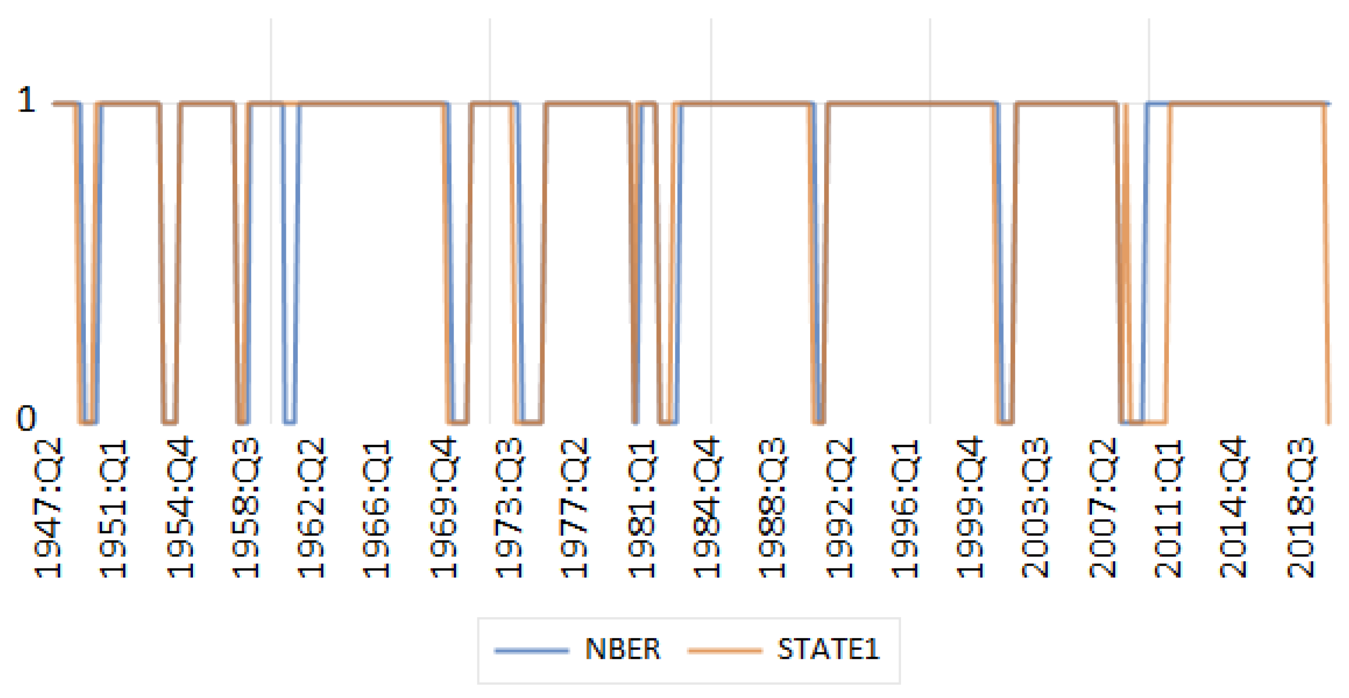
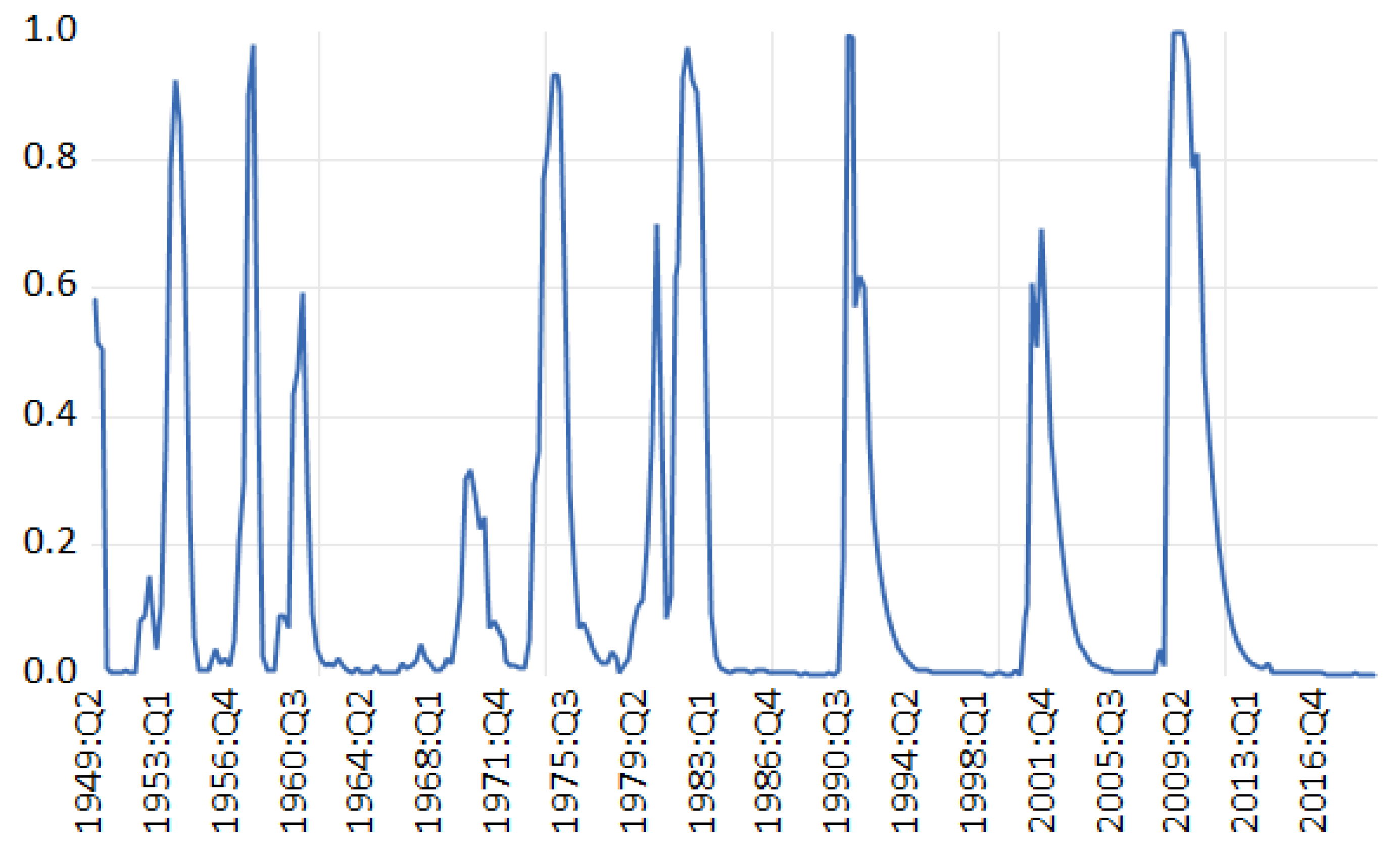
2.2.3. Romer and Romer (2020) on Upgrading NBER Recession Dates

Romer and Romer (RR) work with a two regime MS model, where $z_t$ is the deviation in some variable representing growth in activity from its “normal” level. Thus if one takes log of $GDP$ as the activity variable, the normal level is the log of potential $GDP$, and so one is looking at the change in an output gap. Large changes in that variable signal a recession. To capture potential $GDP$ they use the series given by the the Congressional Budget Office (CBO). The MS model is the simple one with no serial correlation and no changes in the regime variances. RR utilize the 2012 chained $GDP$, which is no longer readily available, and so we use the 2017 chained $GDP$ to get real $GDP$. Because the CBO estimates start in 1949:Q1, we begin at that point rather than backcasting it to 1948:Q1 as RR did. The estimates of the MS model from 1949:Q1 to 2019:Q4 are then

$${\mu }_1=0.89,{\mu }_2=-4.83,p_{11}=0.94,p_{22}=0.69,$$

compared to what RR give

$${\mu }_1=0.81,{\mu }_2=-5.16,p_{11}=0.95,p_{22}=0.68.$$

From the estimate of ${\mu }_2$ we see that the second regime is one of a large decline from “normal”, and so it would agree with their modified definition of a recession. They comment that a probability of the second state being greater than 0.8 would be a recession, and that the range between 0.2 and 0.8 is “..more ambiguous and requiring additional judgement” (p. 27). So it is worthwhile asking what the MS model would say about the threshold that produces a good match to a recession, as they define it. Following the same analysis as for Hamilton’s model, we find that, when concordance is the adopted criterion, c = 0.5 is appropriate. Using regime match however produces c = 0.84. To assess the implications of these different thresholds, the simulated data shows that if c = 0.5 is chosen the match of estimated recession states with the correct ones would be 75%. That rises to 90% when c = 0.84 is used.

In Figure 2, considering the estimates of the probability of the Romers’ defined recession regimes, computed from the fitted MS model for the change in the gap between GDP and its normal level, we see that are some issues about finding no recessions in the 1970s, they are borderline in the 1990s, and none in the 2000s and the 1950s. All of these correspond to recessions as identified by the NBER.

3. Determining Regime Match with Three Regimes

3.1. Principles

Locating three regimes in time is much more complex than doing so with only two regimes. There is little sense in choosing some threshold probability like 0.5 to find a regime from the three estimated $E_T\left({\xi }_{jt}\right)$, although there are many papers that have done that. Suppose we found that the smoothed probabilities of the three states at some t were 0.34, 0.33 and 0.33. Then using a $PT$ of 0.5 we would not be able to classify that observation into any regime. Using an $MP$ rule though would lead to the conclusion the first regime occurred at t. Whether one can improve on it to produce a better match to the true states is a more challenging question. We provide one rule that does do this, but there may be others, and at this date we do not have a final solution.

Concordance between any $S_{jt}=1(E_T\left({\xi }_{jt}\right)>$ 0.5) and any ${\xi }_{jt}$ can be computed, but it is not an overall measure, since it basically looks at combining the match of the estimated $j^{\prime }th$ state with ${\xi }_{jt}$ and the estimated “non-j’th” state with the actual “non-j’th” state. $RM$ is a better overall measure as it asks how well each state can be recovered, which is what we are ultimately interested in. Krolzig and Toro (2005) proposed the use of the highest smoothed probability to assign observations to regimes and noted that in 2-state models this rule was equivalent to using Hamilton’s rule of 0.5 $PT$. So the $MP$ rule applied with the $RM$ criterion seems to be a good start. One can then ask whether it can be improved on.

3.2. Examples of Determining Three Regimes

We now consider two models with three regimes. The first is an extension of the Stata 14 two state MS model to handle three types of interest rate rules. The second allows for expansions and two types of recession, as in Eo and Morley (2022).

3.2.1. Three State Interest Rate Rules—A Stata 14 Example

In the Stata 14 manual the two state MS model described above was discarded in favour of a three state rule. Regime 1 still had a negative coefficient on inflation but, for the other two states it was positive, with state 2 having a smaller value than state 3. So one might think of these as weak, moderately strong, and very strong policy on inflation. A problem that emerges in utilizing their reported results arises from their estimated transition probabilities of $p_{31}$ = 0.6178 and $p_{32}$ = 0.3482, as that seems to imply that $p_{33}$ is almost zero. So, once one gets into regime 3, one departs from it very quickly. This looks odd. However, there is always a labelling problem with MS models that can result in multiple maxima to the likelihood, unless one imposes sufficient restrictions to identify the nature of the states. This does not seem to be done with Stata 14. We re-estimated the model using the Stata 14 data with $EViews$ and got transition probabilities of $p_{31}$ = 0.1742, $p_{32}$ = 0.1044 and $p_{33}$ =0.7214, which seem more reasonable. There was a higher likelihood for the $EViews$ estimates. Nevertheless, the three rules still seemed to be the same types as reported in the Stata 14 manual.3

Utilizing the simulated model data it is found that the fractions of times the regimes are recovered with an $MP$ rule are $0.34$, $0.83$ and $0.12$. So it is very hard to recover periods of very strong and weak inflation policy, while moderate policy periods can be better found.

3.2.2. Three State Rule for Recession Types: Eo and Morley (2023)

Eo and Morley (2023) suggested a three state MS model for data from 1947Q2 to pre-covid. They extended this model to include the covid era by allowing for some extra volatility effects. To avoid difficulties simulating from the longer period model we focus on the period from 1947 until 2019.4

$$z_t=a_{0}1({\xi }_t=1)+a_{1}1({\xi }_t=2)+a_{2}1({\xi }_t=3)+\varphi \sum _{j=1}^{5}1({\xi }_{t-j}=3)+\sigma {\epsilon }_t.$$

(2)

Because $1({\xi }_t=1)+1({\xi }_t=2)+1({\xi }_t=3)=1$ we can re-write the above as

$$z_t={\mu }_1+{\mu }_{2}1({\xi }_t=2)+{\mu }_{3}1({\xi }_t=3)+\lambda \sum _{j=1}^{5}1({\xi }_{t-j}=3)+\sigma {\epsilon }_t$$

where ${\mu }_3+5\lambda =0.$ This is the form of the pre-covid data model estimated by Eo and Morley (2023).

To handle some shifting trend effects found in Eo and Morley (2022) they work with $z_t$ as “detrended” growth in $GDP$. There are three regimes. The first regime is referred to as an expansion, while the other two correspond to different types of recessions. Specifically, regime two is an L shaped recession. Since the dependent variable is the growth in detrended $GDP$, the shock has a permanent effect upon the level of $GDP$. In regime three, as the restriction ${\mu }_3+5\lambda =0$ ensures that there is no long run effect of the shock driving ${\xi }_t$ on the level of $GDP$, it is classified as a U shaped recession.

The model is fitted and we use simulation data to construct the binary variable $S_{jt}$ from $E_T\left({\xi }_{jt}\right)$ with some rule. We first ask how well one can recover each of the regimes in history? With the $MP$ rule expansions are recovered quite well, with $90\%$ of the $S_{1t}$ matching the actual expansion state and the recovery for the two types of recessions are 68%. Eo and Morley (2023) (EM) presented figures for $E_T\left({\xi }_{jt}\right)$ and their only reference to a rule was “This probability closely matches the timing of NBER recessions. In particular, for nine of the eleven NBER recessions in the sample, the smoothed probability is well above 50% for most of a given recession” (p. 250). That seems to suggest that a 0.5 $PT$ rule would be recommended by them.

Using the $MP$ allocation we look in Figure 3 at the indicators capturing the NBER and EM recessions. It is clear that the 1960s recession is completely missed by the MS model. What is of greater import is that the “Great Recession” is very poorly captured by it. Moreover, there is a one quarter L shaped recession in 2008:Q1 and then a 9 quarter U shaped recession from 2008:Q3 to 2010:Q3. Consequently, the MS allocation of recession dates starts two quarters after the NBER recession dates and lasts almost a year longer.

The $MP$ rule gives a regime match to the two types of recessions of $67\%$ and $68\%$. Is it possible to improve on the regime match from that found with the $MP$ rule? To look at this we first find a threshold value for the first regime probability by looking at choosing between states 1 and the combination of states 2 and 3, i.e., choosing between expansions and recessions, just as for the two state case discussed above. This gives a threshold of $c_1$ = 0.74 which enables us to allocate the simulated data into expansion and recession states. Then one has to choose between the two recession states. One proceeds in the same way and this gives a threshold for the L shaped recession of $c_2$ = 0.37. Using the latter threshold the match of the resulting $S_{jt}$ to ${\xi }_{jt}$ ($j=2,3)$ now rises to $71\%$ and $69\%$. Consequently, there is some improvement in the match of the L type recessions. There are quite different conclusions from the results with the $MP$ rule and this extended one. For the $MP$ rule the U shaped recessions are in the 1950s and 2008:Q3-2010:Q3.5 With the probabilities estimated from the extended rule there is only a U shaped recession in 2008 to 2010. So these are quite different interpretations of history.

To look more closely at the issue of the “Great Recession” we should note that the NBER do not detrend data when looking for expansions and recessions. They look for turning points in the level of activity. They use a variety of indicators of activity, but if one only had GDP then the peak and troughs in this would be at the same points as the NBER have set as their turning points in the “Great Recession”. Using the EM series, which is cumulated detrended growth, one finds that the average time spent in expansion and contractions are much the same. This is a characteristic of the growth cycle and not the business cycle, as expansions are much longer than recessions in the NBER cycle dates simply due to trend growth.

We therefore need to look at what is subtracted from $GDP$ growth to get the “detrended series” EM use. They treat $GDP$ growth as having a time varying deterministic mean ${\mu }_t$,

$$\Delta y_t={\mu }_t+{\eta }_t,$$

and then form an estimate of ${\mu }_t$ with a 40 quarter moving average of $GDP$ growth.6 Thus

$$\begin{array}{ccc}\hfill {\widehat{\mu }}_t& =& {\displaystyle \frac{1}{40}}\sum _{j=0}^{40}\Delta y_{t-j}\hfill \\ & =& {\displaystyle \frac{1}{40}}\sum _{j=0}^{40}{\mu }_{t-j}+{\displaystyle \frac{1}{40}}\sum _{j=0}^{40}{\eta }_{t-j}.\hfill \end{array}$$

So ${\widehat{\mu }}_t$ does not recover ${\mu }_t$ but an average of all the deterministic terms over the past 40 quarters. ${\mu }_t$ is never recovered, simply the 40 quarter average of them. So while there has been structural change in the growth rate, it has not been fully removed when one uses $z_t=\Delta y_t-{\widehat{\mu }}_t.$ Note that an extra term has also been added to the error ${\eta }_t$, namely ${\displaystyle \frac{1}{40}}{\sum }_{j=0}^{40}{\eta }_{t-j}$. This augments any existing serial correlation and certainly affects standard errors. The EM series ${\widehat{\mu }}_t$ is presented in Figure 4 as $DEM$. Some of the issues that arise with the very long duration of the “Great Recession” in their estimates appear likely to come from this way of allowing for any shift in potential growth rates, and one might want to work with alternative ways of handling any such shifts.

In that vein we could ask if there is a different measure of “trend” available? The same issues arose in the Romer and Romer application discussed in the last section. They estimated ${\mu }_t$ with the CBO potential output level. Figure 5 compares that to what EM use, and clearly there are some similarities and differences. Perhaps a different way to see the latter is to regress the CBO potential growth rate on $\Delta y_{t-1},\dots ,\Delta y_{t-40}$—the coefficients are double (1/40) in the early weights.

Fitting the EM model with $z_t$ being the growth in $GDP$ less the CBO potential growth rate one finds that there are no longer any L shaped recessions in response to the shock ${\xi }_t,$ only U shaped ones.7 Figure 5 shows the probability of the latter over the period. Given that the estimated MS model says there are only expansions and U shaped recessions we ask what the threshold value for the probability of a U shaped recession would be when using the regime match criterion. It turns out to be 0.81, so Figure 5 shows that there are only six recessions (in the sense of the Romer and Romer definition) signalled in the post war period. Using that threshold, 82% of the expansions and 90% of the U shaped recessions would be recovered from simulations of the model.

4. Locating Regimes When There Are More Series than Regimes

Suppose we have M series. One can assemble information about recurrent events from data on each one. Then some questions arise—is there a common recurrent event or are we just interested in producing some account that summarizes the recurrent event information coming from the data on the individual series? We look at these issues in the case where a MS model captures the common recurrent event.

With two series following a MS process that is common to both we would have

$$\begin{array}{ccc}\hfill z_{1t}& =& {\mu }_{11}{\xi }_t+{\mu }_{12}(1-{\xi }_t)+{\sigma }_1{\epsilon }_{1t}\hfill \end{array}$$

(3)

$$\begin{array}{ccc}\hfill z_{2t}& =& {\mu }_{21}{\xi }_t+{\mu }_{22}(1-{\xi }_t)+{\sigma }_2{\epsilon }_{2t}\hfill \end{array}$$

(4)

where ${\epsilon }_{jt}$ are $n.i.d.(0,1)$ and represent idiosyncratic components. So the Hidden Layer Markov Chain ${\xi }_t$ is an AR(1) whose parameters and shocks depend only upon the transition probabilities. The observed processes can be different depending on the values of ${\mu }_{j1}$ and ${\mu }_{j2}$ and the idiosyncratic component. Because one only wants a common recurrent event it would seem to make sense in an experiment that one sets ${\mu }_{11}={\mu }_{21}={\alpha }_1$ and ${\mu }_{12}={\mu }_{22}={\alpha }_2$ and only allow the idiosyncratic component ${\sigma }_j{\epsilon }_{jt}$ to vary. Then the common recurrent event is ${\alpha }_1{\xi }_t+{\alpha }_2(1-{\xi }_t)$. We assume that for each series one has an accounting of where the regimes are in its history, i.e., we have a set of $E_T({\xi }_{jt}$) or $S_{jt}$ and the issue is how to settle upon a set of regimes to characterize any common component. To look at this one needs to have a common recurrent event and, in keeping with the orientation of this paper, we will assume that it is a MS process as above. We therefore want to combine the $E_T({\xi }_{jt}$) or $S_{jt}$ in order to provide a strong match with the events ${\xi }_t=1$ and 0.

What rules might one use? Romer and Romer (2020) formed the average of the smoothed probabilities $E_T({\xi }_{jt}$) found by fitting MS processes to each series and compared this to some c to decide on which aggregate regime one was in. In the experiment below c = 0.5. A simple rule advocated by Krolzig and Toro (2005), which is used by many institutions such as the European Central Bank and International Monetary Fund, is to say that regime one holds if more than $x\%$ of the $S_{jt}$ are unity at $t.$ Normally $x=50.$ Thus one sums the $S_{jt}$ (which are binary) and compares that to the integer immediately below $M/2$.8

If one had (say) fitted an MSVAR model to all M series imposing a single recurrent event MS process one could check the performance of the rules above (and others) in locating the common regimes. This is not often done. Here we work with a given common MS process where the ${\alpha }_1$ and ${\alpha }_2$ come from US GDP growth, as does ${\sigma }_1.$ Nine series are generated. Variation between the series is due to the idiosyncratic term, ${\sigma }_j{\epsilon }_{jt}$ being different. The random numbers ${\epsilon }_{jt}$ are different to ${\epsilon }_{1t}$ for $j>1.$ The ${\sigma }_j$ are multiples of ${\sigma }_1$ where the factors of proportionality $b_j$ are randomly chosen from a uniform (0,1) random variable. In this case we find that both rules perform extremely well with recovery of over 99% of both regimes. In order to introduce some more variation we allowed ${\mu }_{j1}$ and ${\mu }_{j2}$ to vary as ${\mu }_{j1}=b_j{\alpha }_1$ and ${\mu }_{j2}=b_j{\alpha }_2.$ The regime recovery rates are now $96.3\%$ and $98.7\%$ for the Krolzig and Toro rule, and $96.7\%$ and $99.0\%$ for the Romer and Romer rule. So it seems that one can recover aggregate outcomes quite well with either rule.

5. Conclusions

The paper has looked at where regimes hold in history after the fitting of a Hidden Layer Markov Chain. From that exercise one gets the estimated smoothed probability of a regime holding at any point in time, but to decide whether a particular regime has occurred requires some threshold rule applied to the probabilities. Often researchers use some value that seems most probable to them. Thus, in a two state Markov chain this is generally 0.5. For three states the most common rule is to take the regime that has the highest probability. We argue that there is information in the fitted model that can be used to select a threshold. Specifically, we propose a regime matching criterion and find what thresholds maximize this. Examples are provided to show that the threshold found in this way can better recover the regimes and it can result in quite different allocations of regimes in history. It is easy to do the computation and the information provided can reveal how robust are the conclusions drawn from the model.

References

1. Candelon, B., Dumitrescu, E.-I., & Hurlin, C. (2012). How to evaluate an early-warning system: Toward a unified statistical framework for assessing financial crises forecasting methods. IMF Economic Review, 60(1), 75–113. [Google Scholar] [CrossRef]
2. Chahrour, R., & Jurado, K. (2022). Recoverability and expectations-driven fluctuations. The Review of Economic Studies, 89(1), 214–239. [Google Scholar] [CrossRef]
3. Douwes-Schultz, D., Schmidt, A. M., Shen, Y., & Buckeridge, D. (2023). A three-state coupled Markov switching model for COVID-19 outbreaks across Quebec based on hospital admissions. arXiv, arXiv:2302.02488. [Google Scholar]
4. Eo, Y., & Morley, J. (2022). Why has the US economy stagnated since the Great Recession? Review of Economics and Statistics, 104(2), 246–258. [Google Scholar] [CrossRef]
5. Eo, Y., & Morley, J. (2023). Does the Survey of Professional Forecasters help predict the shape of recessions in real time? Economics Letters, 233, 111419. [Google Scholar] [CrossRef]
6. Hamilton, J. D. (1989). A new approach to the economic analysis of nonstationary time series and the business cycle. Econometrica, 57(2), 357–384. [Google Scholar] [CrossRef]
7. Harding, D., & Pagan, A. (2006). Synchronization of cycles. Journal of Econometrics, 132(1), 59–79. [Google Scholar] [CrossRef]
8. Harding, D., & Pagan, A. (2016). The econometric analysis of recurrent events in macroeconomics and finance. Princeton University Press. [Google Scholar]
9. Krolzig, H.-M., & Toro, J. (2005). Classical and modern business cycle measurement: The European case. Spanish Economic Review, 7, 1–21. [Google Scholar] [CrossRef]
10. Martínez-Beneito, M. A., Conesa, D., López-Quílez, A., & López-Maside, A. (2008). Bayesian Markov switching models for the early detection of influenza epidemics. Statistics in Medicine, 27(22), 4455–4468. [Google Scholar] [CrossRef] [PubMed]
11. Pagan, A., & Robinson, T. (2022). Excess shocks can limit the economic interpretation. European Economic Review, 145, 104120. [Google Scholar] [CrossRef]
12. Rodriguez Palenzuela, D., Grigoraș, V., Saiz, L., Stoevsky, G., Tóth, M., & Warmedinger, T. (2024). The euro area business cycle and its drivers. (Tech. Rep.). European Central Bank Occasional Paper No. 354. Available online: https://www.econstor.eu/handle/10419/301916 (accessed on 1 February 2025).
13. Romer, C. D., & Romer, D. H. (2020). NBER recession dates: Strengths, weaknesses, and a modern upgrade. Mimeo. [Google Scholar]
14. Shaby, B. A., Reich, B. J., Cooley, D., & Kaufman, C. G. (2016). A Markov-switching model for heat waves. The Annals of Applied Statistics, 10(1), 74–93. [Google Scholar] [CrossRef]
15. StataCorp. (2015). Stata 14: Time series reference manual. Stata Press College Station. [Google Scholar]
16. Twain, M. (1903). The jumping frog (illustrated by f. strothman). Harper and Brothers. [Google Scholar]
17. Yang, L., Lahiri, K., & Pagan, A. (2024). Getting the ROC into Sync. Journal of Business & Economic Statistics, 42(1), 109–121. [Google Scholar]
Figure 1. Probability of the Weak Inflation Rule (PROB1) with thresholds of c = 0.5 (CRITP5) and c = 0.35 (CRITP35). Quarterly data from 1955:Q3 to 1979:Q4.
Econometrics 13 00009 g001
Figure 2. Probability of Romers’ Recession (PROB2) and the RM Maximized Threshold of 0.84 (PCRIT). Quarterly data from 1949:Q1 to 2019:Q4.
Econometrics 13 00009 g002
Figure 3. Comparison of NBER expansions (NBER = 1) and EM expansions (State1 = 1). Quarterly data from 1947:Q2 to 2019:Q4.
Econometrics 13 00009 g003
Figure 4. Estimates of Changing Trend Growth in GDP by EM (DEM) and using the CBO data (DCBOPOT). Quarterly data from 1949:Q2 to 2019:Q4.
Econometrics 13 00009 g004
Figure 5. Probability of U-shaped recessions from the EM model using the CBO data. Quarterly data from 1949:Q2 to 2019:Q4.
Econometrics 13 00009 g005
Disclaimer/Publisher’s Note: The statements, opinions and data contained in all publications are solely those of the individual author(s) and contributor(s) and not of MDPI and/or the editor(s). MDPI and/or the editor(s) disclaim responsibility for any injury to people or property resulting from any ideas, methods, instructions or products referred to in the content.