Exponential Time Trends in a Fractional Integration Model

Abstract

This paper introduces a new modelling approach that incorporates nonlinear, exponential deterministic terms into a fractional integration framework. The proposed model is based on a specific test on fractional integration that is more general than the standard methods, which allow for only linear trends.. Its limiting distribution is standard normal, and Monte Carlo simulations show that it performs well in finite samples. Three empirical examples confirm that the suggested specification captures the properties of the data adequately.

1. Introduction

It is common practice in applied work to allow for simple linear deterministic trends when modelling standard economic and financial series (Bhargava 1986; Stock and Watson 1988; Schmidt and Phillips 1992). However, some of these appear to be characterised by exponential growth, as in the case of compound interest. An exponential growth trend can be captured through taking logs of the series of interest and regressing the data against a constant and a linear trend. However, fitting a linear trend with a constant growth rate is in most cases too restrictive. Alternatively, the raw data can be used to run a regression including an exponential time trend as well as a constant. The present paper takes the latter approach based on exponential trends and develops an appropriate modelling and testing framework in the context of fractional integration with a standard normal asymptotic distribution. The proposed fractional integration model belongs to the category of long-memory processes; its feature is that the number of differences that are required to make a series stationary and with short memory (e.g., a white noise or a stationary ARMA) is a non-integer positive value. In most cases investigated with such models, a linear trend is considered and most of the departures from this specification are in the form of special non-linear deterministic structures such as those produced by Chebyshev polynomials in time or Fourier functions. This paper considers exponential trends instead and employs simulation techniques to evaluate the properties of the proposed test with finite samples; it also presents three empirical applications to show that the advocated framework captures well the behaviour of the data. Modelling exponential trends in a fractional integration framework is a novel contribution, and the suggested approach is a practical tool to use in cases of economic and financial series that possibly exhibit long memory as well as exponential deterministic trends.

The structure of this paper is as follows. Section 2 presents the proposed framework and testing procedure along with its asymptotic distribution, which is standard normal. Section 3 reports some Monte Carlo simulation results to assess the finite sample behaviour of the suggested test. Section 4 discusses three empirical applications. Section 5 offers some concluding remarks.

2. The Model

We consider a time series {y_t, t = 1, 2, …. } for which the following regression model is specified:

$$y_t=\alpha +\beta t^{\gamma }+x_t,\hspace{0.17em}\hspace{0.17em}\hspace{0.17em}\hspace{0.17em}\hspace{0.17em}t=1,\hspace{0.17em}2,\hspace{0.17em}\dots ,$$

(1)

where α, β and γ are unknown parameters (the intercept, the time trend coefficient and its exponent respectively); in addition, x_t is assumed to be an integrated process of order d, i.e.,:

$${(1-B)}^d{x}_t=u_t,\hspace{0.17em}\hspace{0.17em}t=1,\hspace{0.17em}2,\hspace{0.17em}\dots ,$$

(2)

where d can be any real scalar value, B is the backshift operator, i.e., B^kx_t = x_t−k, and u_t is thus an I(0) process, more precisely a covariance–stationary one with a spectral density function that is positive and bounded at all frequencies in the spectrum.1 Thus, u_t might be a white noise process but it might also display a weakly autocorrelated structure as in the autoregressive moving average (ARMA) processes.

We test the null hypothesis:

$$H_o:d=d_o,$$

(3)

for any real value d₀ in the model given by (1) and (2), through choosing specific values for γ, for example between 0 and 2, with 0.01 increments. Under the null hypothesis (3), the model given by (1) and (2) becomes:

$${\tilde{y}}_t=\alpha {\tilde{1}}_t+\beta ({\tilde{t}}_t{)}^{ }+u_t, t=1,2,...,$$

(4)

where

$${\tilde{y}}_t={(1-B)}^{d_o}{y}_t,$$

and2

$${\tilde{1}}_t=(1-B{)}^{d_o}1,\hspace{1em} \mathrm{and} {\tilde{t}}_t=(1-B{)}^{d_o}(t{)}^{\gamma },$$

and u_t is still an I(0) process. Since the value of γ is set, one can follow the same strategy as in Robinson (1994) and therefore the test statistic is given as follows:

$$\widehat{r}=\frac{\sqrt{T}}{{\widehat{\sigma }}^2}\frac{\widehat{a}}{\sqrt{\widehat{A}}},$$

(5)

where T is the sample size, and

$$\widehat{a}=\frac{-2\pi }{T}{\sum }_j^{*}\psi \left({\lambda }_j\right)g_u\left({\lambda }_j\widehat{; \tau }{)}^{-1}I\right({\lambda }_j); {\widehat{\mathrm{\sigma }}}^2={\mathrm{\sigma }}^2(\widehat{\mathrm{\tau }})=\frac{2\mathrm{\pi }}{\mathrm{T}}{\displaystyle \sum _{\mathrm{j}=1}^{\mathrm{T}-1}{\mathrm{g}}_{\mathrm{u}}{({\mathrm{\lambda }}_{\mathrm{j}};\widehat{\mathrm{\tau }})}^{-1}\hspace{0.17em}\mathrm{I}({\mathrm{\lambda }}_{\mathrm{j}})},$$

$$\widehat{A}=\frac{2}{T}\left({\displaystyle \sum _j^{*}\psi ({\lambda }_j)\psi ({\lambda }_j)\prime -}{\displaystyle \sum _j^{*}\psi ({\lambda }_j)\widehat{\epsilon }({\lambda }_j){\left({\displaystyle \sum _j^{*}\widehat{\epsilon }({\lambda }_j)\hspace{0.17em}\widehat{\epsilon }({\lambda }_j)\prime }\right)}^{-1}{\displaystyle \sum _j^{*}\widehat{\epsilon }({\lambda }_j)\hspace{0.17em}\psi ({\lambda }_j)}\prime \hspace{0.17em}}\right);$$

$$\psi \left({\lambda }_j\right)=\mathit{log} \left|2\mathit{sin} \frac{{\lambda }_j}{2}\right|; \widehat{\epsilon }\left({\lambda }_j\right)=\frac{\partial }{\partial \tau }\mathit{log} g_u\left({\lambda }_j\widehat{; \tau }\right),$$

where λ_j = 2πj/T and the summation in * in the above equations is over all frequencies which are bounded in the spectrum.3 I(λ_j) is the periodogram of ${\widehat{u}}_t\hspace{0.17em},$ where

$${\widehat{u}}_t={\tilde{y}}_t-\widehat{\alpha }{\tilde{1}}_t-\widehat{\beta }({\tilde{t}}_t{)}^{ }, t=1,2,...,$$

(6)

$\widehat{par}=\left(\begin{array}{c}\widehat{\alpha }\\ \widehat{\beta }\end{array}\right)\hspace{0.33em}\hspace{0.33em}={\left({\sum }_{t=1}^T{\tilde{z}}_t^T{\tilde{z}}_t\right)}^{-1}{\sum }_{t=1}^T{\tilde{z}}_t{\tilde{y}}_t,$ ${\tilde{z}}_t=\left({\tilde{1}}_t, {\tilde{t}}_t\right)$^T, and $\widehat{\tau }\hspace{0.17em}\hspace{0.17em}\hspace{0.17em}\hspace{0.17em}\hspace{0.17em}=$$\hspace{0.17em}\arg \hspace{0.17em}\hspace{0.17em}{\min }_{\tau \hspace{0.17em}\in \hspace{0.17em}{T}^{*}}\hspace{0.17em}{\sigma }^2(\tau )\hspace{0.17em},$ with T^* as a suitable subset of the R^q Euclidean space. Finally, g_u is a known function coming from the spectral density of u_t:

$$f_u(\lambda )\hspace{0.17em}\hspace{0.17em}\hspace{0.17em}=\hspace{0.17em}\hspace{0.17em}\hspace{0.17em}\frac{{\sigma }^2}{2\hspace{0.17em}\pi }\hspace{0.17em}{g}_u(\lambda ;\tau ),\hspace{0.17em}\hspace{0.17em}\hspace{0.17em}-\pi <\lambda \hspace{0.17em}\le \pi .$$

Note that this test is parametric and, therefore, it requires specific modelling assumptions about the short-memory specification of u_t. In particular, if u_t is a white noise, g_u ≡ 1, whilst if it is an AR process of the form φ(L)u_t = ε_t, (with white noise ε_t), then g_u = |φ(e^iλ)|⁻², with σ² = V(ε_t) and the AR coefficients being a function of τ.

In this context, Robinson (1994) showed that for γ = 1:

$$\widehat{R}={\widehat{r}}^2 {\to }_d {\chi }_1^2, as T \to \infty ,$$

(7)

where “→_d” stands for convergence in distribution. Therefore, unlike in the case of other (unit root/fractional) procedures, this is a classical large-sample testing situation. On the basis of (5), the null H_o (3) is rejected against the alternative H_a: d ≠ d_o if $\widehat{R}$ > ${\chi }_{1,\alpha }^2$, with Prob (${\chi }_1^2$ > ${\chi }_{1,\alpha }^2$) = α. In addition, one-sided tests can be obtained against the alternatives H_a: d > d_o (d < d_o) at the 100α% when $\widehat{r}$ > z_α ($\widehat{r}$ < −z_α), where the probability that a standard normal variate exceeds z_α is α.

This result holds for any finite value of γ. Specifically, Robinson (1994) used the following regression model:

$$y_t=\beta {z_t}^{ }+x_t, t=1,2,...,$$

(8)

where z_t is a (kx1) observable vector whose elements are assumed to be non-stochastic, such as polynomials in t, for example, to include the null hypothesis of a unit root with drift if d_o = 1 and z_t = (1, t)^T. According to Robinson: “The limiting null and local distributions of our test statistic are unaffected by the presence of such regressors. For simplicity, we treat only linear regression, but undoubtedly a nonlinear regression will also leave our limit distributions unchanged, under standard regularity conditions”. These regularity conditions are described in his definition of the class G provided in Appendix A to that paper: “G is the class of k X 1 vector sequences { z_t, t = 0, +1, …} such that z_t = 0, t < 0 and D defined as:

$$D\hspace{0.33em}\hspace{0.33em}={\sum }_{t=1}^T{\tilde{w}}_t {\tilde{w}}_t^T, and{{ {\tilde{w}}_t^T}_{ }}_{ }=({\tilde{1}}_t, {\tilde{t}}_t)$$

(9)

is positive definite for sufficiently large T.”. G imposes no rate of increase on D; different elements can increase at different rates, and indeed D need not tend to infinity as T → ∞. If D is positive definite for T = T_o, then it is positive definite for all T > T_o.

In this context, the following theorem can be stated:

Theorem 1.

Under the null hypothesis (3) in the model defined by Equations (1) and (2), with γ = γ_o where γ_o is the true value of the exponential trend, and under the condition:

$$0<\det \left(\Psi \right)<\infty$$

(10)

where det denotes determinant and $\Psi =\frac{1}{2\pi }{\int }_{-\infty }^{\infty }{\psi \left({\lambda }_j\right)}^2$, $\widehat{r}$ converges asymptotically in distribution:

$$\widehat{r}\underset{d}{\to } N(0, 1) \mathrm{as} T \to \infty$$

(11)

Note that the right-hand-side inequality in (10) is not satisfied by the autoregressive AR alternatives, whilst it is by the fractional model in (2) (see the expression for $\psi \left({\lambda }_j\right)$ below (5), and Appendix A for the proof of this theorem).

As an alternative approach, one can compute the residual sum of the squares for a set of values of γ and choose the one that minimises it. In such a case, under standard regularity conditions, the estimate should coincide with the one obtained with our method when choosing the value of d that minimises $\widehat{\widehat{R}}$ in (11). In the empirical applications carried out in Section 4, we set values of γ = 0, 0.10, 0.20, … (0.10), …, 1.40, and 1.50, and in each case we estimated the differencing parameter via choosing the test statistic (based on Robinson 1994) with the lowest value. The estimate of d was virtually identical to the Whittle one based on the frequency domain analysed in Robinson (1994), as $\widehat{\widehat{R}}$ clearly depends on γ. Then, for each value of γ and the associated d, we computed the residual sum of the squares and chose the pair producing the lowest statistic, $\widehat{R}$, in (7).

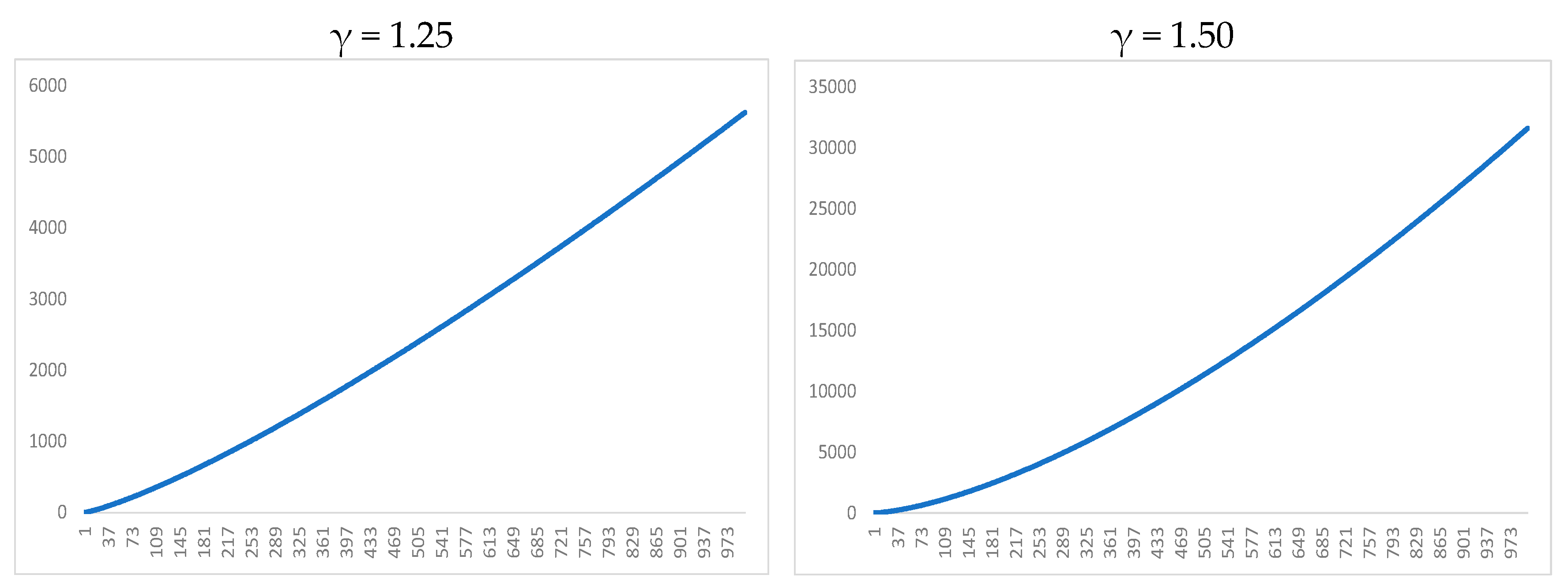
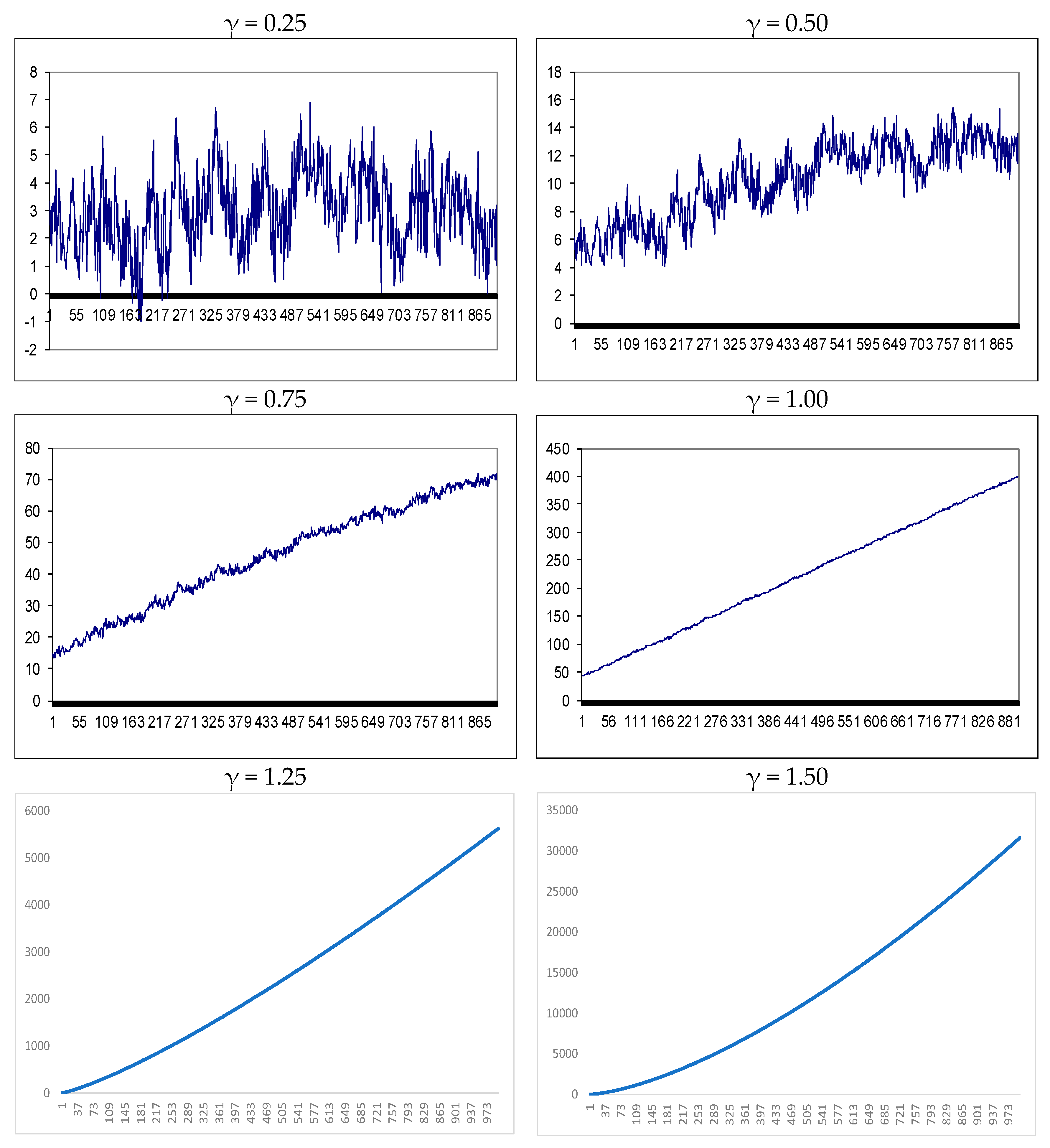
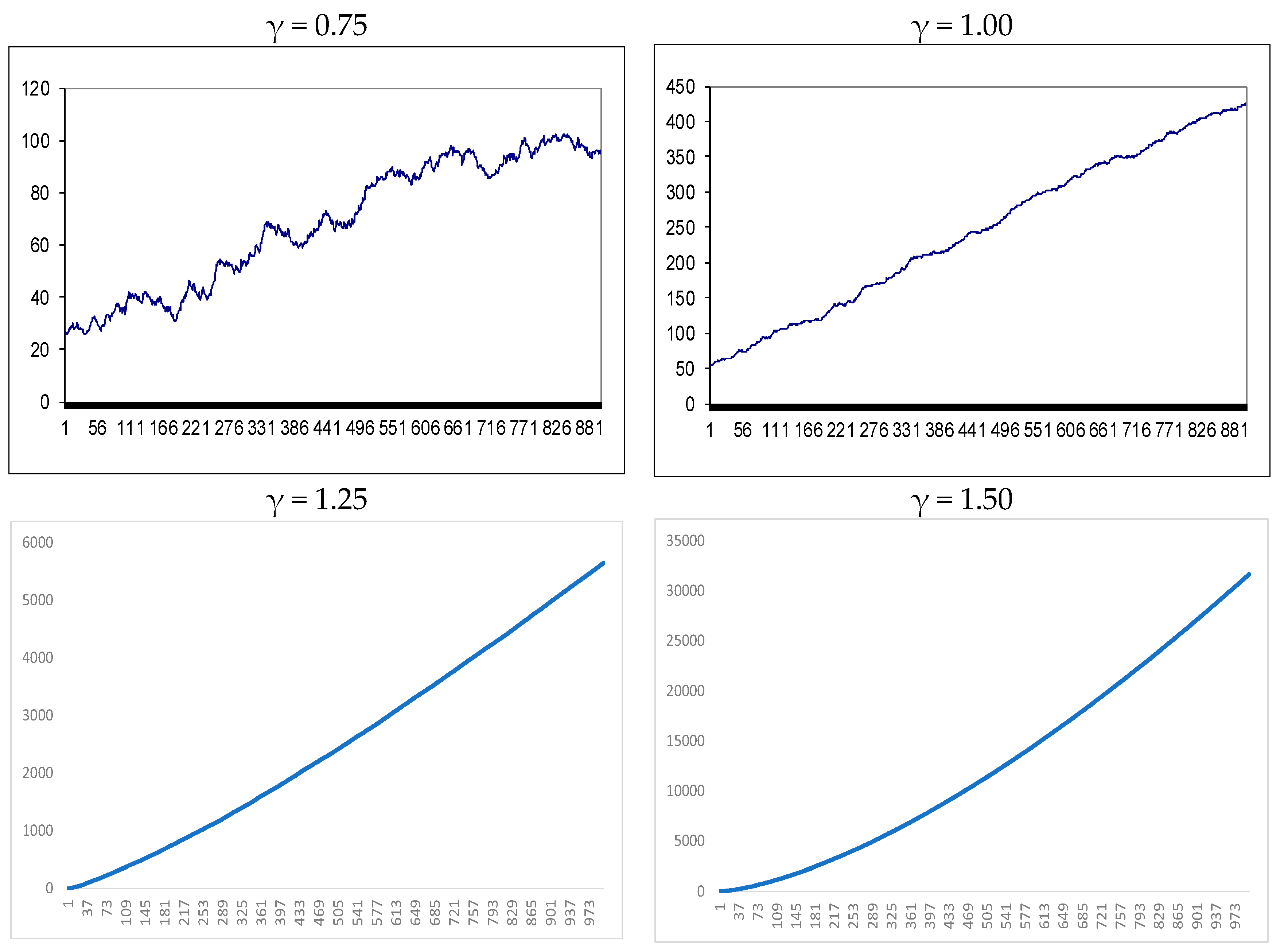
Next, we display some realisations of the model given by Equations (1) and (2). More specifically, we first generated a white noise process with sample size T = 1000, and produced time series for ${\tilde{1}}_t\hspace{0.17em}\hspace{0.17em}\hspace{0.17em}$ and ${\tilde{t}}_t$ via setting different values for d₀ and γ. Then, ${\tilde{y}}_t\hspace{0.17em}$ was obtained from Equation (4) with α = 0.2 and β = 0.4 and first differences of d₀ were taken after removing the first 100 observations.

Figure 1, Figure 2, Figure 3 and Figure 4 correspond to d_o = 0.25, 0.50, 0.75, and 1 respectively, and each of them includes plots of the series (i.e., y_t in (1) and (2)) for γ = 0.25, 0.50, 0.75, 1, 1.25, and 1.50. It can be seen that when γ = 0.25, the trend was almost unnoticeable; however, as γ increased the series exhibited a clear trend characterised by convexity, whilst γ = 1 corresponded to a linear trend, and γ > 1 to one exhibiting concavity.

3. Simulation Results

In this section, we examine the finite sample behaviour of the test statistic proposed above by means of Monte Carlo simulation techniques (the Fortran codes are available from the authors upon request). As data generating processes, we used the GASDEV and RAN3 routines from Press et al. (1986) to obtain Gaussian series for different sample sizes T = 100, 500, and 1000 and carried out 10,000 replications in each case; specifically, we used the model given by Equations (1) and (2) with α = 0.2 and β = 0.4, γ = 0.75, and tested the null hypothesis (3) with d_o = 0.50; the reported results are for a nominal size of 5%. Using alternative values for α, β, γ, and d_o produced almost identical results.

Table 1. Rejection frequencies against one-sided alternatives with Gaussian errors.

	do	T = 100	T = 500	T = 1000
Ho: d > do	0.20	0.688	0.983	1.000
	0.30	0.478	0.688	0.808
	0.40	0.296	0.354	0.499
	0.50	0.099	0.069	0.057
Ho: d < do	0.50	0.104	0.099	0.068
	0.60	0.319	0.449	0.676
	0.70	0.665	0.883	0.997
	0.80	0.997	1.000	1.000

Note: The values reported in this table are the rejection frequencies of the test against fractional alternatives. The size of the test is shown in bold.

displays the rejection frequencies of the test statistic $\widehat{r}$ in (5) for three different sample sizes, T = 100, 500, and 1000 and a nominal size of 5%.4 It can be seen that the nominal sizes were too large in all cases, and they approached 0.05 as the sample size increased. There was also a bias in the size as higher values were obtained in all cases against alternatives of form d < d_o. Finally, the frequencies against departures from the null increased as the sample size increased, which was consistent with the asymptotic behaviour in the test.

Table 2. Rejection frequencies against one-sided alternatives with t₃-distributed errors.

	do	T = 100	T = 500	T = 1000
Ho: d > do	0.20	0.709	0.878	0.998
	0.30	0.526	0.735	0.910
	0.40	0.314	0.359	0.651
	0.50	0.112	0.089	0.067
Ho: d < do	0.50	0.127	0.109	0.083
	0.60	0.414	0.565	0.712
	0.70	0.727	0.899	1.000
	0.80	1.000	1.000	1.000

Note: The values reported in the table are the rejection frequencies of the test against fractional alternatives. The size of the test is shown in bold.

is similar to Table 1 but reports the results based on the t₃-Student distribution for the error term. Once again, the sizes were higher than the 5% level and higher values were observed against departures in the form d < d_o. The rejection frequencies were also higher for this type of departure, and even for small ones the rejection frequencies were relatively high.

4. Three Empirical Applications

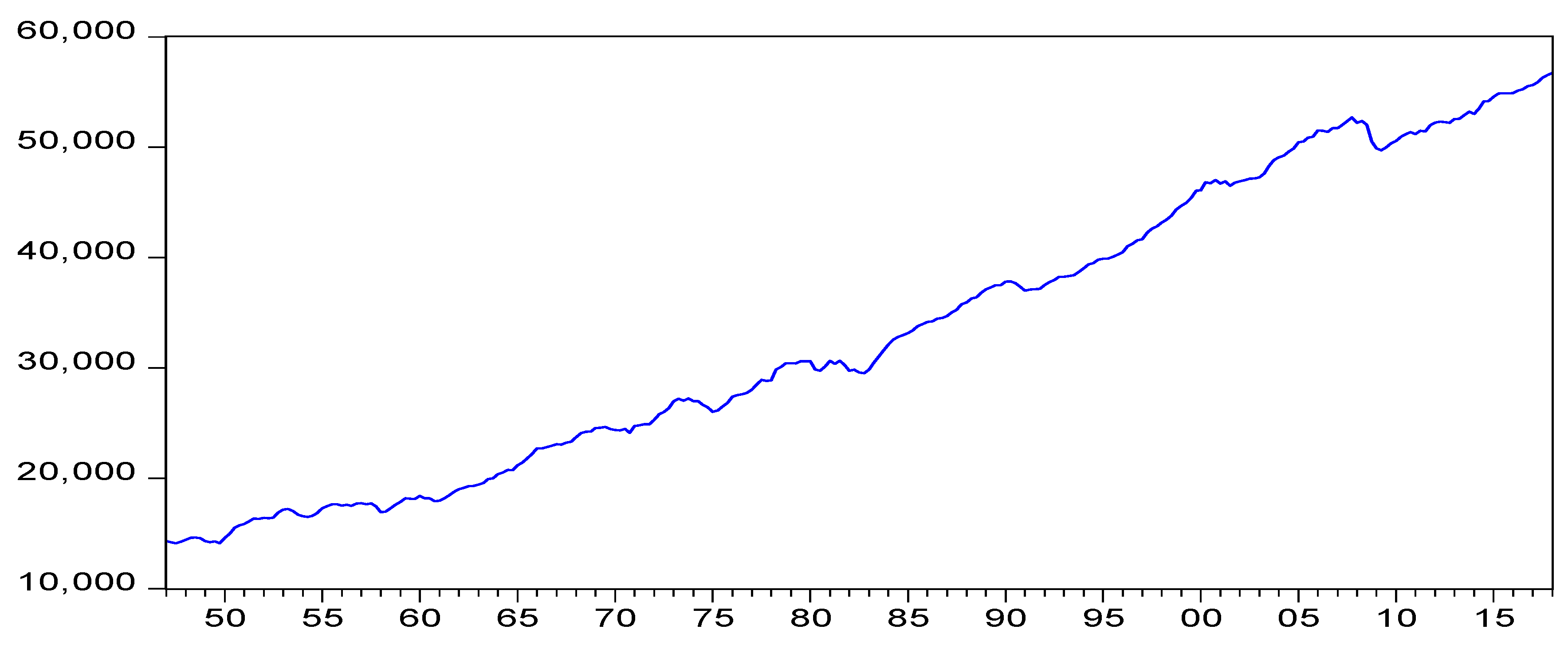
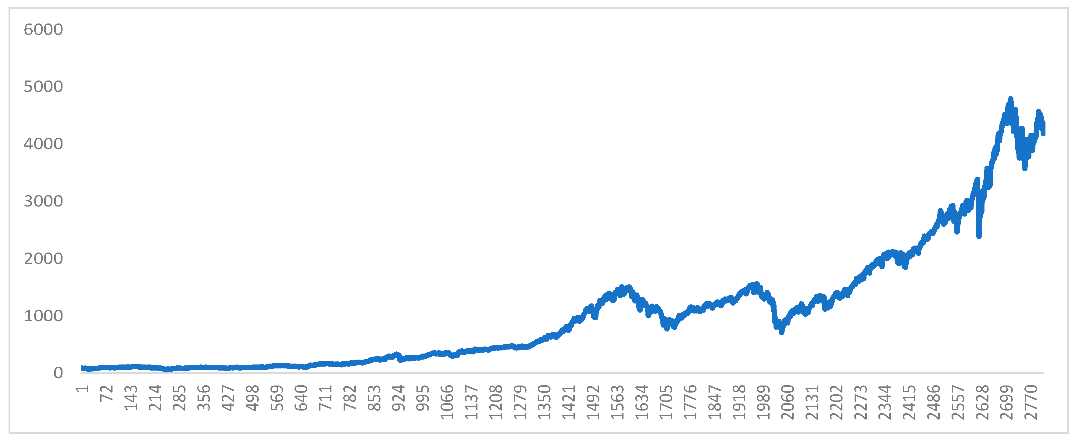
For illustration purposes, we used the proposed framework to model three US time series. The first was the US real GNP per capita series analysed in Omay et al. (2017); it is quarterly and spans the period from 1947 Q1 to 2018 Q1, for a total of 285 observations (see Figure 5), and its source was the FRED database of the Federal Reserve Bank of St Louis (https://www.stlouisfed.org/ accessed on 1 May 2020). The second was the S&P500 weekly series from 1 January 1970 up to 23 October 2023, obtained from Yahoo! Finance (see Figure 6). The third was the US Consumer Price Index for All Urban Consumers, monthly, from January 1913 until October 2023 (see Figure 7). The issue of interest is whether the effects of exogenous shocks are transitory or permanent, and thus whether the series can be characterised as trend stationary or difference stationary (Omay et al. 2017).

Table 3. Estimated coefficients for the log of US real GNP per capita.

Γ	d	95% Band	α (t-Value)	β (t-Value)	Stastistic
0	1.29	(1.18, 1.42)	9.568 (1120.32)	---	0.02218
0.10	1.29	(1.18, 1.43)	9.625 (80.19)	−0.00584 (−0.47)	0.04994
0.20	1.29	(1.18, 1.43)	9.585 (172.36)	−0.01811 (−0.31)	0.04412
0.30	1.29	(1.18, 1.43)	9.572 (299.66)	−0.00473 (−0.13)	0.03298
0.40	1.29	(1.18, 1.43)	9.565 (404.95)	0.00347 (0.14)	0.00959
0.50	1.29	(1.18, 1.43)	9.561 (550.26)	0.00823 (0.46)	0.02218
0.60	1.29	(1.17, 1.42)	9.559 (712.56)	0.01068 (0.83)	-0.05273
0.70	1.28	(1.17, 1.42)	9.559 (882.03)	0.01165 (1.33)	0.05811
0.80	1.28	(1.17, 1.42)	9.561 (1008.38)	0.00981 (1.68)	0.00337
0.90	1.28	(1.17, 1.42)	9.583 (1079.09)	0.00709 (1.92)	0.01557
1.00	1.28	(1.17, 1.42)	9.565 (1107.19)	0.00453 (2.04)	0.01978
1.10	1.28	(1.17, 1.42)	9.567 (1115.28)	0.02653 (2.05)	0.05558
1.20	1.29	(1.18, 1.42)	9.567 (1119.87)	0.00147 (1.91)	-0.03381
1.30	1.29	(1.19, 1.42)	9.568 (1119.53)	0.00079 (1.83)	0.02787
1.40	1.30	(1.19, 1.42)	9.568 (1122.12)	0.00041 (1.63)	-0.06320
1.50	1.30	(1.20, 1.43)	9.568 (1121.49)	0.02166 (1.54)	-0.01687

Note: The first column reports the values of the exponent for the trend. The second and third columns, respectively, refer to the estimated differencing parameter and the associated 95% confidence intervals. The following columns display the intercept and the slope of the exponential trend along with their associated t-values. The final column reports the test statistics.

reports the results for US real GNP, more precisely, the estimates of α, β, γ, and d in the model given by Equations (1) and (2) under the assumption that u_t is a white noise process with zero mean and constant variance. It can be seen that when values of γ from 0 to 1.50 with 0.10 increments were selected, the estimates of d were very similar and ranged from 1.28 to 1.30. The estimated model exhibited an exponential trend with γ = 0.80, d = 1.28, and the 95% confidence interval being given by (1.17, 1.42), with the remaining two parameters, α and β, both being statistically significant. Thus, the unit root null hypothesis is rejected in favour of d > 1 and γ < 1, which indicates the presence of a concave time trend in the data.

Table 4. Estimated coefficients for the S&P500 stock market prices.

Γ	d	95% Band	α (t-Value)	β (t-Value)	Stastistic
0	0.96	(0.93, 1.02)	41.119 (0.171)	---	0.227
0.10	0.96	(0.93, 1.02)	42.633 (0.143)	49.836 (0,16)	0.219
0.20	0.97	(0.92, 1.23)	52.366 (0.399	39.924 (0.31)	0.203
0.30	0.97	(0.92, 1.23)	54.121 (0.70)	37.914 (0.56)	0.239
0.40	0.95	(0.91, 1.22)	57.445 (1.09)	34.327 80.90)	0.202
0.50	0.95	(0.91, 1.22)	59.009 (1.18)	34.327 (0.90)	0.200
0.60	0.96	(0.92, 1.22)	73.080 (1.99)	18.523 (1.71)	0.188
0.70	0.97	(0.92, 1.23)	80.733 (2.28)	10.997 (2.08)	0.161
0.80	0.97	(0.92, 1.23)	85.950 (2.46)	5.941 (2.38)	0.091
0.90	0.97	(0.92, 1.23)	89.053 (2.55)	3.004 (2.62)	0.006
1.00	0.97	(0.92, 1.22)	90.718 (2.60)	1.461 (2.81)	−0.001
1.10	0.97	(0.92, 1.23)	91.577 (2.63)	0.693 (2.96)	−0.154
1.20	0.98	(0.92, 1.22)	92.010 (2.64)	0.324 (3.09)	−0.225
1.30	0.97	(0.92, 1.23)	92.228 (2.65)	0.149 (3.20)	−0.289
1.40	0.98	(0.93, 1.23)	92.341 (2.65)	0.068 (3.30)	−0.346
1.50	0.97	(0.92, 1.24)	92.042 (2.61)	0.031 (3.39)	−0.398

Note: The first column reports the values of the exponent for the trend. The second and third columns, respectively, refer to the estimated differencing parameter and the associated 95% confidence intervals. The following columns display the intercept and the slope of the exponential trend along with their associated t-values. The final column reports the test statistics.

has the same layout as the previous one but concerns the S&P500 stock market index. The estimates of d ranged between 0.91 and 1.24 and the lowest statistic was obtained with γ = 1.00 and d = 0.97 (0.92, 1.24). Thus, a linear time trend with a unit root seems to be a plausible hypothesis; this is consistent, for t > 2, with a random walk model with an intercept, and thus with the efficiency market hypothesis (EMH) in its weak form (Fama 1970).

Finally,

Table 5. Estimated coefficients for the US Consumer Price Index.

Γ	d	95% Band	α (t-Value)	β (t-Value)	Stastistic
0	1.43	(1.36, 1.51)	9.921 (3.13)	---	0.144
0.10	1.43	(1.36, 1.51)	9.938 (1.71)	−0.144 (−0.02)	0.147
0.20	1.42	(1.36, 1.50)	9.851 (3.60)	−0.056 (−0.01)	0.129
0.30	1.43	(1.36, 1.52)	9.814 (5.81)	−0.018 (−0.03)	0.122
0.40	1.43	(1.35, 1.52)	9.784 (8.36)	−0.015 (−1.21)	0.124
0.50	1.42	(1.37, 1.50)	9.871 (4.44)	−0.017 (−1.22)	0.108
0.60	1.43	(1.36, 1.51)	9.742 (4.26)	0.123 (−0.02)	0.119
0.70	1.42	(1.36, 1.50)	9.796 (7.88)	0.125 (0.59)	0.114
0.80	1.43	(1.37, 1.52)	9.475 (5.76)	0.166 (0.60)	0.094
0.90	1.44	(1.38, 1.52)	9.697 (24.36)	0.171 (0.87)	0.088
1.00	1.44	(1.37, 1.50)	9.722 (26.15)	0.151 (1.11)	0.079
1.10	1.44	(1.38, 1.52)	9.755 (26.85)	0.106 (1.32)	−0.055
1.20	1.44	(1.38, 1.50)	9.780 (27.05)	0.064 (1.91)	−0.079
1.30	1.44	(1.37, 1.51)	9.741 (27.11)	0.034 (1.93)	−0.087
1.40	1.44	(1.38, 1.51)	9.799 (26.14)	0.018 (1.98)	−0.119
1.50	1.44	(1.37, 1.51)	9.801 (27.13)	0.009 (1.65)	−0.145

Note: The first column reports the values of the exponent for the trend. The second and third columns, respectively, refer to the estimated differencing parameter and the associated 95% confidence intervals. The following columns display the intercept and the slope of the exponential trend along with their associated t-values. The final column reports the test statistics.

reports the corresponding results for the US Consumer Price Index. In this case, d was much higher than 1 (specifically, 1.44), with a confidence interval given by (1.38, 1.52). Thus, the unit root null hypothesis is rejected in favour of d > 1; also, the estimate of γ = 1.10 implies a convex time trend.

5. Conclusions

This paper puts forward a long-memory modelling and testing framework that allows for exponential deterministic trends in a fractional integration context. An attractive feature of the proposed test statistic is that its asymptotic distribution is N(0,1). The Monte Carlo simulations carried out to examine the properties of the proposed test indicated that it performed well with finite samples. As an illustration, the proposed framework was then applied to model the behaviour of US real GDP, the S&P500 stock market index, and US consumer prices. The empirical exercise showed that the suggested model captured well the behaviour of the series under examination and was data-congruent; specifically, in the case of US real GNP per capita and US CPI, the exponential trend fractional model outperformed the one with a linear trend (i.e., γ = 1) for different differencing parameters.

The proposed modelling approach is widely applicable to time series that exhibit exponential trends. However, it should be noted that, although unlimited exponential growth might characterise some economic and financial series, this is not likely to occur whenever real resources are involved. In such cases, there will necessarily be an upper bound which should also be introduced into the model, for instance, through a logistic curve. In addition, the stochastic structure of the model described with Equation (2) can be extended using alternative approaches that allow for poles or singularities in the spectrum at one or more frequencies away from zero, as is the case with seasonal and/or cyclical structures.5 These issues are left for future research.

References

1. Bhargava, Alok. 1986. On the Theory of Testing for Unit Roots in Observed Time Series. The Review of Economics Studies 53: 369–84. [Google Scholar] [CrossRef]
2. Brown, Bruce M. 1971. Martingale central limit theorems. Annals of Mathematical Statistics 53: 59–66. [Google Scholar] [CrossRef]
3. Fama, Eugene F. 1970. Efficient Capital Markets: A Review of Theory and Empirical Work. Journal of Finance 25: 383–417. [Google Scholar] [CrossRef]
4. Gil-Alana, Luis A. 1997. Testing of Fractional Integration in Macroeconomic Time Series. Ph.D. thesis, London School of Economics, LSE, London, UK. [Google Scholar]
5. Gil-Alana, Luis A. 2001. Testing Stochastic Cycles in Macroeconomic Time Series. Journal of Time Series Analysis 22: 411–30. [Google Scholar] [CrossRef]
6. Gil-Alana, Luis A., and Peter M. Robinson. 2001. Testing of seasonal fractional integration in UK and Japanese consumption and income. Journal of Applied Econometrics 16: 95–114. [Google Scholar] [CrossRef]
7. Omay, Tolga, Rangan Gupta, and Giovanni Bonaccolto. 2017. The US real GNP is trend stationary after all. Applied Economics Letters 24: 510–14. [Google Scholar] [CrossRef]
8. Press, William H., Saul A. Teukolsky, William T. Vetterling, and Brian P. Flannery. 1986. Numerical Recipes. The Art of Scientific Computing. Cambridge: Cambridge University Press. [Google Scholar]
9. Robinson, Peter M. 1991. Testing for strong serial correlation and dynamic conditional heteroskedasticity in multiple regression. Journal of Econometrics 47: 67–84. [Google Scholar] [CrossRef]
10. Robinson, Peter M. 1994. Efficient tests of nonstationary hypotheses. Journal of the American Statistical Association 89: 1420–37. [Google Scholar] [CrossRef]
11. Schmidt, Peter, and Peter CB Phillips. 1992. LM tests for a unit root in the presence of deterministic trends. Bulletin of Economcis and Statistics 53: 257–87. [Google Scholar] [CrossRef]
12. Stock, James H., and Mark W. Watson. 1988. Variable Trends in Economic Time Series. Journal of Economic Perspectives 2: 147–74. [Google Scholar] [CrossRef]
13. Tanaka, Katsuto. 1999. Nonstationary fractional unit root. Econometric Theory 15: 549–82. [Google Scholar] [CrossRef]
14. Yaya, Olaoluwa, Ahamuefula Ogbonna, Luis Alberiko Gil-Alana, and Fumitaka Furuoka. 2021. A new unit root analysis for testing hysteresis in unemployment. Oxford Bulletin of Economics and Statistics 83: 960–81. [Google Scholar] [CrossRef]
Figure 1. Realisations from Equations (1) and (2) with d = 0.25. Note: We generated Gaussian series with T = 1000, and then produced the realisations of yt in (1) and (2) with d = 0.25.
Econometrics 12 00015 g001aEconometrics 12 00015 g001b
Figure 2. Realisations from Equations (1) and (2) with d = 0.50. Note: We generate Gaussian series with T = 1000, and then produce the realisations of yt in (1) and (2) with d = 0.50.
Econometrics 12 00015 g002
Figure 3. Realisations from Equations (1) and (2) with d = 0.75. Note: We generated Gaussian series with T = 1000, and then produced the realisations of yt in (1) and (2) with d = 0.75.
Econometrics 12 00015 g003
Figure 4. Realisations from Equations (1) and (2) with d = 1.00. Note: We generated Gaussian series with T = 1000, and then produced the realisations of yt in (1) and (2) with d = 1.00.
Econometrics 12 00015 g004aEconometrics 12 00015 g004b
Figure 5. US real GNP per capita. Note: the data source was the FRED database of the Federal Reserve Bank of St Louis (https://www.stlouisfed.org/ accessed on 1 May 2020); the series is quarterly and the sample period spans from 1947 Q1 to 2018 Q1.
Econometrics 12 00015 g005
Figure 6. S&P500 Stock Market Index. Note: the data source was Yahoo! Finance (https://es.finance.yahoo.com/); the series is weekly and the sample period extends from 1 January 1970 to 23 October 2023.
Econometrics 12 00015 g006
Figure 7. US Consumer Price Index for All Urban Consumers. Note: the data source was the U.S. Department of Labor Bureau of Labor Statistics (https://www.bls.gov); the series is monthly and the sample period runs from 1913m1 to 2023m10.
Econometrics 12 00015 g007