Financial and Oil Market’s Co-Movements by a Regime-Switching Copula

Abstract

Over the years, oil prices and financial stock markets have always had a complex relationship. This paper analyzes the interactions and co-movements between the oil market (WTI crude oil) and two major stock markets in Europe and the US (the Euro Stoxx 50 and the SP500) for the period from 1990 to 2023. For that, I use both the time-varying and the Markov copula models. The latter one represents an extension of the former one, where the constant term of the dynamic dependence parameter is driven by a hidden two-state first-order Markov chain. It is also called the dynamic regime-switching (RS) copula model. To estimate the model, I use the inference function for margins (IFM) method together with Kim’s filter for the Markov switching process. The marginals of the returns are modeled by the GARCH and GAS models. Empirical results show that the RS copula model seems adequate to measure and evaluate the time-varying and non-linear dependence structure. Two persistent regimes of high and low dependency have been detected. There was a jump in the co-movements of both pairs during high regimes associated with instability and crises. In addition, the extreme dependence between crude oil and US/European stock markets is time-varying but also asymmetric, as indicated by the SJC copula. The correlation in the lower tail is higher than that in the upper. Hence, oil and stock returns are more closely joined and tend to co-move more closely together in bullish periods than in bearish periods. Finally, the dependence between WTI crude oil and the SP500 stock index seems to be more affected by exogenous shocks and instability than the oil and European stock markets.

1. Introduction

Energy prices play an important role in economic activity and growth, which can impact stock markets. One of the major consequences of that is the financialization of the commodity market. This phenomenon has been highlighted, particularly in the last decade, and has been the main driver of commodity price developments since the early 2000s. It was caused by an expansion of commodity transactions by investors and financial institutions in derivatives markets. This expansion of commodities can be attributed to different reasons. The first one is for investors to diversify their portfolios and minimize losses and risks related to their investments. This attractive feature of commodities can be attributed to their lack of correlation with other financial assets. Jones and Kaul (1996); Chong and Miffre (2010), Lescaroux and Mignon (2008), Gorton and Rouwenhorst (2006), and Buyuksahin et al. (2010) have confirmed the negative or even independent relationship between commodities and other traditional financial assets such as equities, stocks, and bonds. The second reason for this expansion is the huge increase in trading and speculation with commodities. Consequently, they were massively included in portfolios, not just for diversification benefits but also for investment purposes. Progressively, commodities have come to behave like other traditional financial assets as their correlation is no longer the same but has been increasing because of these changes. This is how the financialization of commodities was initiated at the beginning of 2000.

In this paper, I study the conditional correlation and dependency between oil commodity prices and stock market prices (in terms of their volatility) to better understand their relationships and co-movements. Understanding the dynamics of their price behavior would be of interest from a consumer and supplier perspective as well as from a policy perspective. The analysis of dependence and interactions between energy and stock markets and among economic, macroeconomic, and financial variables in general is a matter of great importance. It represents one of the biggest challenges facing researchers, investors, and financial agents. It allows them a better understanding of the economic behavior of price returns and the nature of their linkages and associations. Additionally, it helps them make better decisions in terms of risk management and asset allocation.

This paper focuses on energy commodities, particularly crude oil. Energy commodities represent a major class of commodities. In addition, they play a major role in economic development, international trade, and global economic and political stability. Hence, they have been particularly affected by commodity trading (the financialization) during the last decade. Consequently, their association with financial markets has been strengthened. During the global crisis, in particular, there was a dramatic increase in the correlation between crude oil and other equities and stock returns, as the collapse of prices also affected energy commodities. In this paper, I consider the oil commodity. First, it is one of the fundamental inputs of the economies of many countries, such as the US, on the production and/or consumption sides. Second, because oil market trading activity is the highest among other energy commodities.

Generally, the dependence between variables is measured using the Pearson correlation coefficient. However, this indirectly assumes the hypothesis of both normality and linearity of the returns, which is not the case, particularly for financial data. When faced with this non-linearity, non-normality, and some other features characterizing financial data, such as heavy tails, asymmetry, leverage, and extreme events, returns need to be modeled using a much more flexible and non-standard model—a model capable of incorporating these features and going beyond the linear approach to appropriately evaluate and examine the dependence structure. In this context, the copula approach is the best alternative for overcoming these limitations. It is a mathematical and statistical tool that was introduced by Sklar (1959). It allows us to properly model the joint distributions of multiple variables and examine their conditional correlations and co-movements in more detail.

Copulas are of interest to statisticians for two main reasons: as a way of studying scale-free measures of dependence and as a starting point for constructing families of bivariate and multivariate distributions. It was Embrechts et al. (1999) that introduced copula functions into financial econometrics in a seminal work. Meanwhile, it was pioneered by Patton (2006) as one of the most powerful and useful tools to model and measure the dependence and correlation between asset returns and financial data.

In this paper, I analyze the dynamics of the relationship and co-movements between the WTI crude oil price and two major stock prices (SP500 for the US financial market and Euro Stoxx 50 for the European stock market). To this end, I model their joint distribution using the time-varying (dynamic) copula introduced by Patton (2006). The dependence parameter, which describes the evolution of the correlation, is time-varying. In addition, the intercept term of the dependence equation depends on a hidden first-order Markov chain. This model represents the regime-switching (RS) copula, a model in which the dynamic process can undergo sudden shifts in regimes. It was proposed by da Silva Filho et al. (2012). The choice of this particular model for studying dependence is not random. In finance, the dependence between financial asset returns is often subject to instability and shifts over time. A well known example of such shifts and instability used in this paper corresponds to the idea of bull and bear regimes alternating in financial markets. Thus, with the particular case of the RS copula model, I aim to detect visible and persistent swings in trends between the oil and US/European stock markets. Furthermore, regime-switching models are the best candidates for representing and capturing more complex nonlinear dynamic patterns, such as asymmetry. The Markov switching model is suitable for describing correlated data that exhibits distinct dynamic patterns during different periods Kuan (2002). The performance of the RS copula model was compared to the dynamic copula without incorporating Markov regime switching in order to prove its efficiency in capturing the dependence structure, taking into account the breaks and regimes over the period of the study. The number of studies dealing with regime switching in copula functions is limited. Also, the dependence was treated as constant and not dynamic in most cases (Jondeau and Rockinger 2006; Rodriguez 2007; Chollete et al. 2009; Fei et al. 2013). More recently, researchers include Boubaker and Sghaier (2016), Fink et al. (2017), Pircalabu and Benth (2017), and Zhou (2019), among others.

Estimating the copula parameter is crucial but demanding. The dependence parameter incorporates an unobserved process variable related to the regime-switching model. Consequently, it is not straightforward and computationally intensive to evaluate the log-likelihood of the studied model. To proceed with the estimation process, I use Kim’s filter method, proposed by Kim and Nelson (1999), to obtain the smoothing probabilities and evaluate the likelihood function together with the usual inference function for margins (IFM) method for copula estimation.

Attention will be directed to the marginals, which must also be modeled and estimated properly since they represent the first step in obtaining copula inputs. As proposed by Engle (1982), Bollerslev (1986), and Creal et al. (2013), I consider a GARCH (generalized autoregressive conditional heteroskedasticity)/GAS (generalized autoregressive score) approach to model the returns. Then, standardized residuals of each variable were extracted, and the empirical cumulative distribution function ‘ecdf’ was applied to transform them into uniform data for copula inputs.

The major findings of this paper are presented as follows: The dependence of WTI crude oil with the SP500 and the Euro Stoxx50 financial indexes has been persistent over time. The RS copula model was a good fit to analyze and measure the dynamics and time evolution of their co-movements by identifying two distinct regimes. The dependence between crude oil and stock returns can be divided into two stages: a relatively calm state and a turbulent state. The calm state corresponds to the low regime, where conditional correlations between the studied variables were weak or negative. The turbulent state corresponds to the high regime during exogenous shocks, crises, news, or turmoil, where dependency increases significantly. With WTI crude oil, both SP500 and Euro Stoxx 50 stock returns exhibited an asymmetric tail correlation due to lower tail correlations being higher than upper tail correlations. In other words, extreme negative returns were more tail-dependent than extreme positive returns. The oil crude with the SP500 and Euro Stoxx 50 indexes were more dependent and linked when extreme negative events occurred than when positive extreme events occurred. However, the US stock market was found to be more affected by exogenous shocks, instability, and bad news than the European stock market.

2. Review of the Literature

Modeling dependence is of great importance for financial and economic applications. The understanding of their relationship and behavior toward each other and the comprehension of their interactions in the financial market have become the focus of attention for many investors, policymakers, and researchers. It has important implications for risk prevention, portfolio selection and optimization, risk management, and asset diversification.

Many authors have confirmed the relationship between oil and stock prices. Sadorsky (1999) argued that oil price volatility had an impact on stock returns. The same applies to the work of Hammoudeh and Li (2008). They suggested that some major events that caused changes in oil prices also tended to increase stock market volatility. Malik and Ewing (2009) used the BEKK-GARCH model to examine the volatility transmission between oil prices and five US sector indices from 1992 to 2008. They showed the existence of a significant transmission of shocks and volatility between oil prices and the studied stock returns. Arouri et al. (2012) did the same thing by focusing on the European stock market. Using the VAR-GARCH model, they showed the presence of significant volatility spillovers between them and oil prices from 1998 to 2009. Creti et al. (2013) revealed that correlations between commodities, including the energy and stock markets, increased significantly during the financial crisis. Aboura and Chevallier (2015), with an asymmetric DCC with one exogenous variable model based on the work of Hamao et al. (1990) and Vargas (2008), confirmed the existence of significant interconnections between data from financial and commodity markets from 1983 to 2013. Martin-Barragan et al. (2015), using wavelet analysis, found that there is a connection between oil and stock markets (UK, Germany, US, Germany, and Japan). This relationship was nonexistent in calm periods and increased in periods of crisis. Hanif et al. (2023) also established the time-varying nature of the co-movements between oil and equities using wavelet analysis.

However, modeling the dependence of asset returns is not very simple and requires some well-developed econometric and statistical tools. The exact knowledge of their laws of probability, as well as their joint distribution, is crucial. It is also important to take into account the non-normality and non-linearity of financial data. Numerous empirical works have discussed this issue Fama and French (1993), Richardson and Smith (1993), Longin and Solnik (2001), Mashal and Zeevi (2002).

Faced with this non-linearity and non-normality, as well as other stylized facts characterizing financial data such as heavy tails, asymmetry, negative Skewness, excess Kurtosis, extreme events, and volatility clustering, returns need to be modeled using a flexible model—a model capable of incorporating all these features and going beyond the linear approach to appropriately model their dependency structure. In this context, we chose the copula approach.

The term copula originates from the verb ‘to couple’, which means linking, to join, or unite. To put it simply, copula functions are “functions that join or couple multivariate distribution functions to their one-dimensional marginal distribution functions” Nelsen (2007). The main point of this approach is the possibility of splitting the multivariate (joint) distribution function into two components: marginal distributions that describe the individual behavior of each series, and a copula function that captures the dependence structure between them. The modeling procedure consists of two steps: First, specify the functional form of the marginal distributions. This allows us to explore in detail stylized facts about the returns individually (using GARCH/GAS models, for example). The next step is to determine an adequate copula function that characterizes the dependence between the variables. Thus, copulas have almost all the information concerning the dependence structure independently of the marginal variables.

Several approaches analyzed the dependence structure between different variables and modeled their joint distributions and volatilities. The generalized autoregressive conditional heteroskedasticity (GARCH) model, the BEKK model by Engle and Kroner (1995), and the dynamic conditional correlation (DCC) model by Engle (2002), among others. A major shortcoming of these models is that conditional correlations follow the same dynamic structure Billio et al. (2006). This imposes common dynamics among all assets, in contrast to copula functions, where dependencies rely only on the data. In addition, DCC and BEKK models might provide a fast and straightforward approach to analyzing smaller datasets; however, the parameters to estimate tend to increase significantly for higher dimensions.

The literature study demonstrates a growing focus on modeling the dependence of financial assets. Analyzing their co-movements to understand their behavior and interactions in the financial market has important implications for risk management. Therefore, the choice of a powerful but flexible approach to study and measure dependency is necessary. Copula functions offer several advantages. They allow the modeling of linear, nonlinear, and dynamic dependencies. The objective of this study is to analyze the dependence between oil commodity prices and stock market prices (in terms of their volatility) to better understand their correlations and co-movements. For that, I used the time-varying Markov regime-switching copula model to detect visible and persistent swings in trends between the oil and US/European stock markets.

In the next two sections, I explain the methodology of the RS copula model, and then I present the empirical study followed by the results before concluding.

3. Materials and Methods

In this section, I consider the Markov switching dynamic copula model based on da Silva Filho et al. (2012), which introduces different regimes or states in the dependence structure of the returns. The estimation of the parameters of the copula is conducted using Kim’s filter for regime switching models. Since it is complex and computationally demanding to estimate all the parameters (the copulas parameters and the marginals’ parameters) together in one step, I use the inference function for margins (IFM) method proposed by Joe and Xu (1996) to evaluate the model in two steps. First, I will provide an introduction to copula functions and their properties.

3.1. Introduction to Copulas Functions

Let $Y\in {\mathbb{R}}^n$ be a random vector. Let $F\left(x\right)$ be the cumulative distribution function (CDF) of Y, i.e.,

$$F\left(y\right)=P(Y_1\le y_1,\cdots ,Y_n\le y_n)$$

Further, we denote $F_1,\cdots ,F_n$ to be the marginal CDF of $Y_1,\cdots ,Y_n$. A copula is a function $C:{[0,1]}^n\to [0,1]$ that verifies the following properties:

• For any $i=1,\cdots ,n$,

  $$C(v_j,v_{-j})=v_j$$

  where

  $$v_{-j}=1$$

  means that all arguments except the $j^{th}$ argument are equal to 1.
• $C\left(v\right)\le C\left(u\right)$ if $v\le u$, where $v\le u$ means that $v_i\le u_i$ for all $i=1,\cdots ,n$.
• C is n-increasing, i.e., for any box $[d,e]\subset {[0,1]}^n$ with non-empty volume, $C\left(\right[d,e\left]\right)>0.$

When there are n variables, C is called the n-copula. A copula can be viewed as a CDF of the n-dimensional random vector V such that $V_i\sim Unif[0,1].$ Based on the Sklar theorem, we can link any multivariate cumulative distribution function to a copula function as the following.

Sklar Theorem

For a random vector Y with CDF F and univariate marginal CDFs $F_1,\cdots ,F_n$, there exists a copula C such that:

$$F(y_1,\cdots ,y_n)=C(F_1\left(y_1\right),\cdots ,F_n\left(y_n\right))$$

If Y is continuous, then such a copula C is unique.

3.2. The Model

The regime-switching (RS) copula model is an extension of the dynamic copula based on Patton (2006) by adding a regime-switching part to the autoregressive dependence equation. Note $Y_t={(y_{1,t},y_{2,t})}^{\prime }$, $t=\left\{1\dots T\right\}$, a bivariate time series vector. By applying the Sklar theorem, the copula model can be expressed as follows:

$$H(y_1,y_2)=C_{{\theta }_t}(F_1\left(y_{1,t}\right|{\mu }_1),F_2\left(y_{2,t}\right|{\mu }_2)).$$

(1)

If $(F_1,F_2)$ are continuous, then the copula can be expressed as:

$$C(u_1,u_2)=H(F_1^{-1}\left(u_1\right),F_2^{-1}\left(u_2\right)),$$

(2)

where ${\theta }_t$ is the copula parameter, $F_1$ and $F_2$ are the distribution functions of the margins and ${\mu }_1$ and ${\mu }_2$ their parameters. H is the joint distribution function of vector $Y_t$, $u_1=F_1\left(y_{1,t}\right|{\mu }_1)$ and $u_2=F_2\left(y_{2,t}\right|{\mu }_1)$ are uniform copula inputs, obtained from the bivariate process $Y={(y_1,y_2)}^{\prime }$. $C_{{\theta }_t}$ is the dynamic Patton copula of the dependence structure, where ${\theta }_t$ evolves over time through the following mechanism:

$${\theta }_t=\Lambda (\omega +\beta {\theta }_{t-1}+\alpha {\Gamma }_t),$$

(3)

where $(\omega ,\beta ,\alpha )$ are the set of interest parameters to be estimated, $\Lambda$ is an appropriate function depending on the choice of the copula function1 and $\Gamma$ is the forcing variable described as follows:

$${\Gamma }_t=\frac{1}{10}\sum _{i=1}^{10}{F}_1^{-1}\left(u_{1,t-i}\right)F_2^{-1}\left(u_{2,t-i}\right)\mathrm{if}\mathrm{elliptical}\mathrm{copula}$$

(4)

$${\Gamma }_t=\frac{1}{10}\sum _{i=1}^{10}\left|u_{1,t-i}-u_{2,t-i}\right|\mathrm{if}\mathrm{archimedean}\mathrm{copula}.$$

(5)

To sum up, the equation characterizing the conditional correlation evolution of the returns corresponds to an intercept, an autoregressive term $\beta {\theta }_{t-1}$, and a forcing variable ${\Gamma }_t$. ${\Gamma }_t$ is expressed by the mean absolute difference between $u_{1,t}$ and $u_{2,t}$ over the ten previous observations when dealing with Archimedian copulas. It is the product of the inverse c.d.f of the two variables in the case of the elliptical copula.

Our aim is to introduce different regimes to take into account the variations and changes that can affect the dependence between the bivariate process $Y_t$ in terms of their volatilities. The regime switching is introduced to the dependence equation, explained above, by allowing the parameter $\omega$ to depend on a hidden, latent state variable $S_t$. $S_t$ takes discrete values $k=\left[1\dots n\right]$. Two states, or regimes, are considered: $S_t=\left\{0,1\right\}$2. The two states represent low/high regimes. $S_t$ follows a Markov chain of order one, irreducible and ergodic, with a $2\times 2$ transition probability matrix P.

$$\left(\begin{array}{cc}P(S_t=0|S_{t-1}=0)& P(S_t=1|S_{t-1}=0)\\ P(S_t=0|S_{t-1}=1)& P(S_t=1|S_{t-1}=1)\end{array}\right)=\left(\begin{array}{cc}{p}_{00}& p_{01}\\ p_{10}& p_{11}\end{array}\right)$$

where $p_{ij}=P\left[S_t=j|S_{t-1}=i\right]$, $\left(i,j\right)\in \left\{0,1\right\}$ are the transition probabilities of $S_t$ given that $S_{t-1}$. They verify the equation $p_{i0}+p_{i1}=1$. The transition matrix drives the random behavior of the state variable and contains only two parameters $(p_{00}$ and $p_{11})$. The improved copula parameter evolves dynamically, as already defined by Patton (2006), and the constant term ($\omega$) switches according to a Markov chain of order one, as follows:

$${\theta }_t^{S_t}=\Lambda ({\omega }^{S_t}+\beta {\theta }_{t-1}+\alpha {\Gamma }_t).$$

(6)

Finally, the distribution function of the bivariate time series process $(y_{1,t},y_{2,t})$ is given by:

$$(y_1,y_2)\propto C_{{\theta }_t^{S_t}}(u_{1,t},u_{2,t}|{\theta }_t^{S_t}).$$

(7)

3.3. The Estimation

The density function, h, of the vector $Y_t$ can be expressed as:

$$h(y_{1,t},y_{2,t})=c_{{\theta }_t^{S_t}}(u_{1,t},u_{2,t}|{\theta }_t^{S_t})\prod _{i=1}^2{f}_{it}\left(y_{it}\right|{\mu }_i).$$

(8)

Its log-likelihood based on the Markov copula model is the following:

$$\begin{array}{ccc}\hfill l(\Psi |Y_t)& =& \sum _{t=1}^{T}log\left(h(y_{1,t},y_{2,t})\right)\hfill \end{array}$$

(9)

$$\begin{array}{ccc}\hspace{1em}& =& \sum _{t=1}^{T}log\left(c_{{\theta }_t^{S_t}}\left((u_{1,t},u_{2,t})\right|{\theta }_t^{S_t})\times \prod _{i=1}^2{f}_{it}(y_{it};{\mu }_i)\right).\hfill \end{array}$$

(10)

It is not straightforward to evaluate the log-likelihood in the previous equation. It is computationally intensive because we have an unobserved process $S_t$ related to the regime-switching model.

For simplification, we proceed to the decomposition of the log-likelihood function into two equations by referring to the inference function for margins (IFM) method proposed by Xu (1996). Using the IFM method, the parameters of the log-likelihood function are estimated in two stages, plus this method is computationally simpler than the maximum likelihood estimation (MLE).

First, we estimate the parameters of the margins (${\mu }_i$, $i=\left\{0,1\right\}$) and then use these estimated parameters to estimate the copula parameters $\left({\theta }_t^{S_t}\right)$. In the first step, the marginal distribution parameters are estimated using the GARCH and GAS models. Thus, the estimation is straightforward since it follows the traditional approach for GARCH models. The difficulty lies in the estimation of the copula parameters because ${\theta }_c^{S_t}$ depends on a non-observable discrete variable $S_t$ that follows a Markov chain of order one. For that, we use Kim’s filter method, proposed by Kim and Nelson (1999).

The log-likelihood function of the RS copula model is given by:

$$l(\Psi |Y_t)=\sum _{t=1}^T\log \left(c_{{\theta }_t^{S_t}}(F_1\left(y_{1t}\right|{\mu }_1),F_2\left(y_{2t}\right|{\mu }_2)|{\theta }_t^{S_t})\prod _{i=1}^2{f}_{it}\left(y_{it}\right|{\mu }_i)\right),$$

(11)

where c is the copula function with parameter ${\theta }_t^{S_t}$, f is the density of the marginal distribution of the returns $y_i$, ${\mu }_i$ is the set of parameters of the marginals, $F_i$ is the cumulative distribution function, and $\Psi =({\theta }_t^{S_t=0},{\theta }_t^{S_t=1},{\mu }_1,{\mu }_2,p_{11},p_{00})$.

Based on the IFM method, we proceed to the decomposition of the log-likelihood function as follows:

$$\begin{array}{ccc}\hfill l(\Psi |Y_t)& =& \sum _{t=1}^{T}log\left(c_{{\theta }_t^{S_t}}(F_1\left(y_{1t}\right|{\mu }_1),F_2\left(y_{2t}\right|{\mu }_2)|{\theta }_t^{S_t})\prod _{i=1}^2{f}_{it}\left(y_{it}\right|{\mu }_i)\right)\hfill \\ \hfill & =& \sum _{t=1}^{T}log{c}_{{\theta }_t^{S_t}}(F_1\left(y_{1t}\right|{\mu }_1),F_2\left(y_{2t}\right|{\mu }_2)|{\theta }_t^{S_t})+\sum _{t=1}^T\prod _{i=1}^{2}log\left(f_{it}\left(y_{it}\right|{\mu }_i)\right)\hfill \\ \hfill & =& \sum _{t=1}^{T}log{c}_{{\theta }_t^{S_t}}(F_1\left(y_{1t}\right|{\mu }_1),F_2\left(y_{2t}\right|{\mu }_2)|{\theta }_t^{S_t})+\sum _{t=1}^{T}log\left(f_{1t}\left(y_{1t}\right|{\mu }_1)\right)+\sum _{t=1}^{T}log\left(f_{2t}\left(y_{2t}\right|{\mu }_2)\right)\hfill \\ \hfill & =& \sum _{t=1}^{T}log{c}_{{\theta }_t^{S_t}}(u_{1,t},u_{2,t}|{\mu }_1,{\mu }_2;{\theta }_t^{S_t})+\sum _{t=1}^{T}log\left(f_{1t}\left(y_{1t}\right|{\mu }_1)\right)+\sum _{t=1}^{T}log\left(f_{2t}\left(y_{2t}\right|{\mu }_2)\right)\hfill \\ \hfill & =& l_c\left({\theta }_t^{S_t}\right)+l_{f_1}\left({\mu }_1\right)+l_{f_2}\left({\mu }_2\right)\hfill \end{array}$$

$l_{f_1}\left({\mu }_1\right)$ and $l_{f_2}\left({\mu }_2\right)$ are the likelihood functions of the marginal distributions of $y_1$ and $y_2$, respectively. In this case, the parameters of each margin are explicitly estimated without any need for sophisticated numerical optimization. However, this does not apply to $l_c\left({\theta }_t^{S_t}\right)$, the copula log-Likelihood. Considering the different states of $S_t$, $l_c\left({\theta }_t^{S_t}\right)$ can be expressed as:

$$\begin{array}{ccc}\hfill l_c\left({\theta }_t^{S_t}\right)& =& \sum _{t=1}^{T}logc(F_1\left(y_{1t}\right),F_2\left(y_{2t}\right)|{\mu }_1,{\mu }_2;{\theta }_t^{S_t})\hfill \\ \hfill & =& \sum _{t=1}^{T}log(\sum _{S_t=0}^{1}c(F_1\left(y_{1t}\right),F_2\left(y_{2t}\right)|{\mu }_1,{\mu }_2;{\theta }_t^{S_t})\hfill \\ \hfill & =& \sum _{t=1}^{T}log(\sum _{S_t=0}^{1}c(F_1\left(y_{1t}\right),F_2\left(y_{2t}\right)|S_t,I_{t-1})Pr\left(S_t\right|I_{t-1}\left)\right)\hfill \end{array}$$

where $I_{t-1}$ is the set of information available prior to time t.

$S_t$, $t\in \left\{0,1\right\}$ are not observable; thus, the MLE approach is not fitted to estimate the parameters ${\theta }_t^{S_t}$ of the copula likelihood $l_c\left({\theta }_t^{S_t}\right)$. Instead, we use Kim’s filter, which combines the Kalman filter with Hamilton’s filter for Markov switching models.

To evaluate $l_c\left({\theta }_t^{S_t}\right)$, it is necessary to calculate the weights $Pr\left(S_t\right|I_{t-1})$ for both states or, more precisely, the filtered probabilities of the unobservable regime $S_t$ given the available information set. Given $I_{t-1}=\left\{Y_1,Y_2,\dots Y_{t-1}\right\}$, the information set up to $t-1$, and the states $\left\{S_t=i,i\in \left\{0,1\right\}\right\}$, the copula likelihood function of $Y_t$ can be rewritten as:

$$\begin{array}{cc}\hfill c(u_{1t},u_{2t})=& P(S_t=0|I_{t-1};{\theta }_t^{S_t}).c(u_{1t},u_{2t}|S_t=0,I_{t-1};{\theta }_t^{S_t})\hfill \\ \hfill & +P(S_t=1|I_{t-1};{\theta }_t^{S_t}).c(u_{1t},u_{2t}|S_t=1,I_{t-1};{\theta }_t^{S_t}).\hfill \end{array}$$

(12)

For $i=\left\{0,1\right\}$, the filtering probabilities of $S_t$ are:

$$\begin{array}{cc}\hfill P(S_t=i|I_t,{\theta }_t^{S_t})=& \left(P(S_t=i|I_{t-1};{\theta }_t^{S_t}).c(u_{1t},u_{2t}|S_t=i,I_{t-1};{\theta }_t^{S_t})\right)/\hfill \\ \hfill & (P(S_t=0|I_{t-1};{\theta }_t^{S_t}).c(u_{1t},u_{2t}|S_t=0,I_{t-1};{\theta }_t^{S_t})\hfill \\ \hfill & +P(S_t=1|I_{t-1};{\theta }_t^{S_t}).c(u_{1t},u_{2t}|S_t=1,I_{t-1};{\theta }_t^{S_t}))\hfill \end{array}$$

(13)

In addition, we obtained the predicted probabilities using the relationship between them and the filtering probabilities:

$$\begin{array}{cc}\hfill P(S_{t+1}=i|I_t,{\theta }_t^{S_t})=& P(S_{t+1}=i|S_t=0,I_t)P(S_t=0|I_t;{\theta }_t^{S_t})\hfill \\ \hfill & +P(S_{t+1}=i|S_t=1,I_t)P(S_t=1|I_t;{\theta }_t^{S_t}).\hfill \end{array}$$

(14)

The filtering process presented above in Equations (13) and (14) represents the filtering algorithm developed by Kim (1994) and Kim and Nelson (1999). By iterating this process, for $t=1\dots T$, we obtain the filtered probabilities $P(S_t=i|I_t;{\theta }_t^{S_t})$, the conditional densities of the copula $c(u_1,u_2|I_{t-1};{\theta }_t^{S_t})$, and the conditional probability distribution of $S_t$ given the information set up to t.

Obtaining the distribution of $S_t$ for the entire sample using the information given by all T observations would be more efficient than simply considering information up to t. Kim’s filter is used to compute the smoothing probabilities, $Pr(S_t=i|I_T)={\sum }_{j=0}^{1}Pr(S_t=i,S_T=j|I_T)$ where $Pr(S_t=i,S_T=j|I_T)$ is obtained based on the filtered probabilities by applying the backward-smoothing process.

For $(i,j)\in \left\{0,1\right\}$, the smoothing probabilities can be expressed as:

$$P(S_t=i|I_T;{\theta }_t^{S_t})=P(S_t=i|I^t;{\theta }_t^{S_t})\times (\frac{p_{i0}.P(S_{t+1}=0|I_T;{\theta }_t^{S_t})}{P(S_{t+1}=0|I_t;{\theta }_t^{S_t})}+\frac{p_{i1}.P(S_{t+1}=1|I_T;{\theta }_t^{S_t})}{P(S_{t+1}=1|I_t;{\theta }_t^{S_t})}).$$

(15)

The backward-smoothing process is described as follows:

1.

We obtain $P(S_t=i|I_t)$, $i\in \left\{0,1\right\}$ for $t=1\cdots T$, which are given by the filtering algorithm.

2.

We initialize the smoothing algorithm in $t=T$ with the filtering probability $P(S_T=i|I_T;{\theta }_t^{S_t})$ and go back recursively.

3.

For each $t=T-1,\dots ,1$, the smoothing probability distribution $P(S_t=i|I_T;{\theta }_t^{S_t})$ is given by Equation (15).

The combination of the two algorithms, the filtering algorithm (to obtain the filtered probabilities) and the backward-smoothing algorithm (presented above for the smoothing probabilities), is called the forward-filtering–backward-smoothing algorithm, which allows the estimation of the parameters needed to maximize the RS copula log-likelihood.

To summarize, the dependence parameter follows a restricted ARMA process that depends on a latent process $S_t$. The state $S_t$ can have two regimes indicated by $S_t=0$ and $S_t=1$. Additionally, $S_t$ follows a first-order Markov chain. This implies that the probability that regime 0 will occur at time t depends solely on the regime at time $t-1$. This is referred to as the transition probabilities. However, we can use the information from current and past observations, combined with the distributions and transition probabilities, to make an inference on the probability of being in each regime. This gives us the filtering probabilities and the conditional probability distribution of $S_t$ given the information set up to time t. We refer to this procedure as the Hamilton filter. It is also possible to determine the distribution of $S_t$ on a specific regime at time t, using all available information, given all T observations. These are the smoothed probabilities. Kim (1994) presented an efficient recursive algorithm, the forward-filtering–backward-smoothing algorithm, which can be applied to compute these smoothed probabilities. The estimation of the time-varying copula and the RS copula models was performed using Matlab software, particularly the Copula toolbox and the Markov-switching copula toolbox.

4. Results

The Data

This analysis was based on the daily spot prices of West Texas Intermediate (WTI) crude oil, a global benchmark for oil, and two major stock indices: the SP500 (Standard and Poor’s 500), representing the US stock market, and the Euro Stoxx 50, representing the European stock market. The West Texas Intermediate (WTI) crude oil prices were extracted from the US Energy Information Agency (EIA), while the SP500 and the Euro Stoxx 50 were from Yahoo Finance. The series data are of daily frequency, comprising the period from 2 January 1990 to 2 January 2023, for a total of 8255 observations. The datasets take into account different turbulences and extreme events in the economy (the Asian crisis between 1997 and 1998, the global financial crisis around 2007–2009, the European debt crisis of 2009–2012, etc.).

The daily returns of each series, $r_t$, were obtained by taking the log difference of the prices, $p_t$, as follows:

$$r_t=\log \left(p_t\right)-\log \left(p_{t-1}\right)$$

(16)

This transformation is required because the evolution of prices is usually non-stationary, and returns help remove the source of this non-stationarity.

Table 1. Descriptive statistics of the returns.

	SP500	WTI Oil	Euro Stoxx 50
Size	8255	8255	8255
Mean	0.000	0.000	0.000
SD	0.011	0.025	0.013
Max	0.109	0.188	0.104
Min	−0.094	−0.406	−0.090
Excess Kurtosis	8.527	14.659	5.138
Skewness	−0.242	−0.646	−0.113
Jarque Bera	20,155 ***	59,835 ***	7309.4 ***
Robust Q (20)	$27.766$	$28.225$	32.810 *
ARCH	217.140	39.027	139.110

Note: *** and * denote statistical significance at 1% and 10% levels, respectively.

summarizes the descriptive statistics of oil price returns and the two stock returns. All returns were stationary. They exhibited negative skewness and ’excess’ kurtosis, while the Jarque–Bera statistic indicated that neither series is unconditionally normal. The three markets did not show a significant trend over the period of study because their means were very small relative to their standard deviations. Based on the robust Ljung–Box statistic, the Euro Stoxx 50 index suggests the presence of temporal dependence in its returns. In addition, the ARCH-LM test rejects the null hypothesis of no presence of ARCH effects for all variables.

The non-normality, possible asymmetry, and presence of heavy tails further confirmed the nonlinearity between returns. Consequently, the particular choice of the copula model integrating a regime-switching model may be a good candidate to deal with dependence in a more general setting and take into account those features characterizing the data.

Marginal Distributions

To study the marginal distributions of the variables, I used the GARCH/GAS-type models with different distributions for the error terms (Normal, Student, or skewed Student) for their variances (volatilities) and the ARMA/ARFIMA model for the means. The estimation of the models was performed using Oxmetrics software. The aim of this section is to extract and correct the volatilities of the returns from the presence of autocorrelation and conditional heteroscedasticity. The choice of the best-fitted model for the data was based on the information criteria, as well as a set of diagnostic tests.

The results of the estimation of the marginal models are given in

Table 2. Parameter estimates of the returns of the variables: WTI oil, SP500, Euro Stoxx 50; p-values are between parentheses.

	SP500	WTI Oil	Euro Stoxx 50
Mean Equation
Cst (M)	0.000563	0.000199	0.000447
	(0.000)	(0.225)	(0.000)
d-Arfima	0.013	−0.065
	(0.761)	(0.003)
AR (1)	0.009	−0.526
	(0.947)	(0.011)
AR (2)	0.783	0.042
	(0.000)	(0.087)
MA (1)	−0.052	0.579
	(0.614)	(0.005)
MA (2)	−0.799	-
	(0.000)	(-)
Variance Equation			0.012
Cst (V) × ${10}^4$	0.009	0.014	0.000
	(0.002)	(0.004)
ARCH (Alpha1)	0.089	0.082	0.104
	(0.000)	(0.000)	(0.000)
GARCH (Beta1)	0.910	0.917	0.994
	(0.002)	(0.000)	(0.000)
Asymmetry			−0.090
			(0.000)
Tail			7.529
			(0.000)
Diagnostic tests
LL	21609.5	15920	20,317.752
AIC	−6.515	−4.799	−6.126
Q (20)	[0.051]	[0.384]	[0.130]
$Q{\left(20\right)}^2$	[0.051]	[0.080]	[0.493]
ARCH 1–10	[0.079]	[0.103]	[0.391]

. The ARFIMA (2, d, 2)-IGARCH (1, 1) with Normal innovations was the best model for the SP500 index, whereas the ARFIMA (2, d, 1)-IGARCH (1, 1) model with Normal innovations was best for WTI crude oil. For the Euro Stoxx 50, the GAS (1, 1) model with skewed Student-t innovation was the best-fitted model. The lagged autoregressive terms (AR(1) and AR(2)) related to the mean equation of the crude oil and the SP500 were, overall, statistically significant at the $1\%$ level. Thus, past observations (past information sets) did impact and affect the returns of the series. Furthermore, the estimates of the ARCH component in the variance equation were statistically significant for the three studied variables. Thus, all of them exhibit significant ARCH effects. In other words, one-period lagged squared shocks could affect the current conditional volatility. Likewise, the significant GARCH coefficients indicate the persistence of the volatility in each market. Both the coefficients of asymmetry and the degree of freedom of the student distribution were significant. Therefore, the distribution of the European stock market was characterized by heavy tails that could be related to a ‘possible’ dependence in the tails when joined to other distributions.

Testing the accuracy of the estimates to ensure the efficiency of the selected models is crucial for our study. Copula inputs must be well specified for better results. At the $5\%$ significance level, the null hypothesis of no autocorrelation was accepted, and there were no remaining ARCH effects in the estimated residuals, as indicated by the Ljung–Box and the ARCH–LM tests. All models were well specified and offered a good fit for the data. To obtain uniform inputs for the copula model, we used the empirical cumulative distribution. The Anderson Darling (AD), the Cramer–von Mises, and the Kolmogorov–Smirnov (KS) tests, presented in

Table 3. Diagnostic tests (p-values) for standard residuals of the three returns: Anderson Darling (AD), Cramer–von Mises (CvM), and Kolmogorov–Smirnov (KS).

	WTI Oil	SP500	Euro Stoxx 50
CvM	1	1	1
KS	0.993	0.941	0.999
AD	1	1	1

, which were used as uniformity tests for the obtained residuals, did not indicate evidence against the uniform [0, 1].

5. Discussion

The next step, after specifying the marginals of each variable and obtaining uniform data for copula inputs, is to proceed to estimate the copula model. The aim of this study is to examine the dependence and co-movements between the oil market (crude oil) and the US/Europe stock markets represented by the SP500 index and the Euro Stoxx index using the copula approach. The results of the estimation for each pair (SP500-WTIoil and Eurostox50-WTIoil) using both the dynamic and RS copula models are given in

Table 4. Estimated parameters of the dynamic copulas for the WTI crude oil/SP500 and the WTI crude oil/Eurostoxx 50 volatilities; standard errors between brackets.

	SP500	and		WTIoil			EuroStoxx50		and	WTIoil
Copula Function						Copula Function
	Normal	Clayton	Gumbel		SJC		Normal	Clayton	Gumbel		SJC
$\omega$	0.002	0.726	0.881	${\omega }_U$	−17.440	$\omega$	0.002	0.715	−0.093	${\omega }_U$	−18.155
	(0.001)	(0.006)	(-)		(0.001)		(0.001)	(0.105)	(0.120)		(0.001)
$\beta$	1.926	1.485	0.181	${\beta }_U$	−0.002	$\beta$	1.940	−1.434	1.468	${\beta }_U$	−0.007
	(0.0279)	(0.0161)	(-)		(0.000)		(0.026)	(0.357)	(0.236)		(0.000)
$\alpha$	0.0840	0.452	−1.127	${\alpha }_U$	−1.566	$\alpha$	0.063	0.461	−0.536	${\alpha }_U$	−4.005
	(0.016)	(0.006)	(-)		(0.000)		(0.012)	(0.056)	(0.055)		(0.000)
				${\omega }_L$	3.926					${\omega }_L$	3.754
					(0.000)						(0.000)
				${\beta }_L$	−2.852					${\beta }_L$	−2.782
					(0.000)						(0.000)
				${\alpha }_L$	−24.998					${\alpha }_L$	−24.766
					(0.000)						(0.000)
LogL	153.517	96.123	61.249		113.245	LogL	112.900	78.832	72.999		85.514
Aic	−4.060	−3.128	−2.221		2.545	Aic	−3.436	−2.713	−2.553		3.114
Bic	17.091	18.023	18.930		44.849	Bic	17.715	18.438	18.571		45.419

,

Table 5. Estimated parameters of the regime-switching (RS) copula for the WTI crude oil/SP500 volatilities, standard errors between brackets.

	Normal	Clayton	Gumbel		SJC
$w_0$	−0.000	0.511	0.165	$w_{0,u}$	−0.002
	(0.001)	(0.034)	(0.006)		(0.015)
$w_1$	0.175	0.070	−0.662	$w_{1,u}$	−9.653
	(0.067)	(0.208)	(0.896)		(0.558)
$\beta$	1.929	0.507	0.511	${\beta }_u$	2.519
	(0.135)	(0.026)	(0.000)		(0.287)
$\alpha$	0.038	−0.118	−1.653	${\alpha }_u$	−8.883
	(0.046)	(0.084)	(0.067)		(1.219)
p	0.944	0.951	0.982	$w_{0,l}$	−0.745
	(2.424)	(0.500)	(0.372)		(0.319)
q	0.952	0.944	0.975	$w_{1,l}$	−16.687
	(0.942)	(1.166)	(0.674)		(6.324)
				${\beta }_l$	−0.561
					(0.490)
				${\alpha }_l$	2.454
					(1.719)
				p	0.951
					(0.393)
				q	0.944
					(1.025)
logL	213.674	182.082	116.705		188.539
AIC	1.277	1.591	2.492		9.527
BIC	43.581	43.896	44.797		80.034

and

Table 6. Estimated parameters of the regime-switching (RS) copula of the WTI crude oil/Euro Stoxx 50 volatilities; standard errors between brackets.

	Normal	Clayton	Gumbel		SJC
$w_0$	1.656	0.202	0.730	$w_{0,u}$	0.418
	(0.422)	(0.110)	(2.276)		(1.238)
$w_1$	0.003	−1.220	5.417	$w_{1,u}$	−9.386
	(0.067)	(0.080)	(78.249)		(2.634)
$\beta$	1.448	0.572	0.044	${\beta }_u$	1.897
	(0.840)	(0.028)	(1.954)		(0.785)
$\alpha$	0.296	−0.268	−1.813	${\alpha }_u$	−11.224
	(0.122)	(0.245)	(0.563)		(6.771)
p	0.950	0.940	0.933	$w_{0,l}$	0.469
	(0.494)	(1.113)	(56.003)		(0.686)
q	0.942	0.949	0.944	$w_{0,l}$	−24.363
	(1.262)	(0.560)	(1.293)		(87.805)
				${\beta }_l$	−4.107
					(0.129)
				${\alpha }_l$	2.645
					(2.710)
				p	0.951
					(0.380)
				q	0.943
					(0.937)
logL	161.173	145.833	51.763		150.347
AIC	1.837	2.046	4.136		9.978
BIC	44.141	44.351	46.440		80.486

.

Different families of copulas were considered to account for the different characteristics in the dependence structure of the studied variables (linear correlation coefficient, upper/lower tail dependency): Normal, Clayton, Gumbel, and Symmetrized Joe Clayton (SJC). The choice of the best model fitted to the data was based on the maximization of the log-likelihood (or the minimization of the BIC/AIC criteria). For both the time-varying and the regime-switching models, the Normal copula, followed by the SJC copula, was best fitted to describe the dependence of the variables under analysis.

The results of the parameter estimates for the two studied pairs given by the time-varying dynamic copula model (Table 4) show that the autoregressive coefficient in the dependence equation ($\beta$) was overall high for the best-fitted model. Thus, there was a high degree of persistence in the dependence between WTI crude oil and both the US and European stock indices. The parameter estimate, $\omega$, the constant of the copula parameter that reflects the dependency level, was higher with SP500-WTIoil than with Eurostoxx50-WTIoil. Thus, the US stock market had the highest dependency on oil prices compared to the European stock market. The SJC copula describes the behavior of the dependence structure for both the lower and upper tails, which is why it has two different estimates for the constant $\omega$: ${\omega }_L$ and ${\omega }_U$. 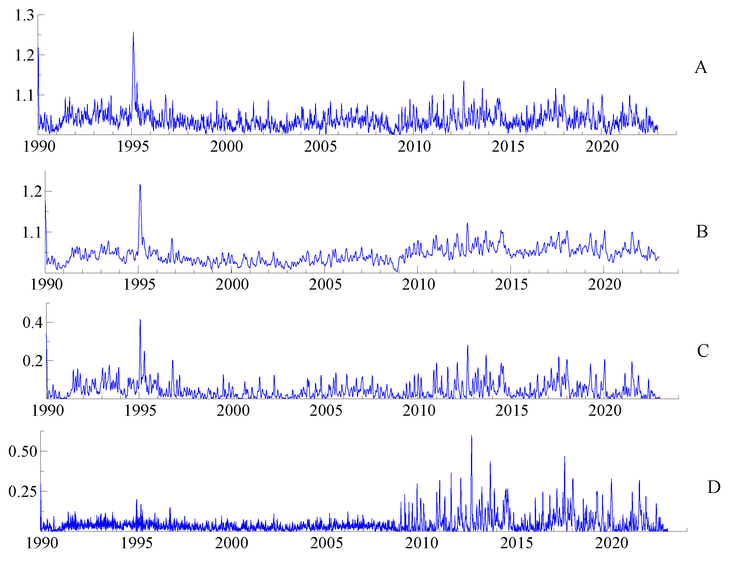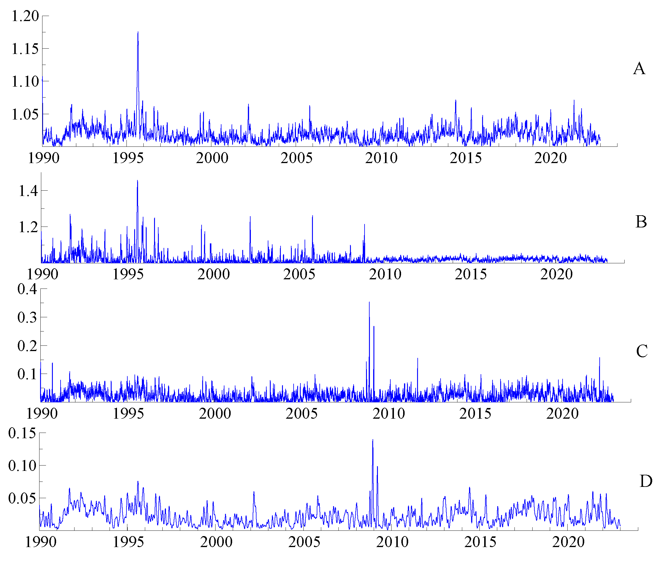For both pairs, ${\omega }_L$ was higher than ${\omega }_U$, meaning that lower-tail correlations are more important than upper-tail correlations for SP500-WTIoil and Eurostoxx50-WTIoil. In other words, the oil-stock extreme dependence differs during the upturn and downturn periods. Negative returns were more dependent than positive returns between US/European stock markets and WTI crude oil. They exhibited asymmetry in extreme dependency. We also confirm this fact based on their time-varying tail dependence given by the dynamic SJC copula model (Figure 1A,C and Figure 2A,C). Indeed, both stock indices reflected more joint negative extremes than joint positive extremes with the WTI crude oil returns. For both pairs, lower-tail correlations took values between 0 and 1.2, while upper-tail correlations did not exceed 0.2. Correlations in the upper tail were very low and weak compared to those in the lower tails, confirming an asymmetric tail dependency with WTI crude oil for both stock indices, particularly the European index, and the nonlinearity of their dependency. Aloui et al. (2013) used the copula approach and also confirmed asymmetry in extreme comovements between crude oil and equity markets in the case of the Central and Eastern European transition economies.

Table 5 and Table 6 report the parameter estimates of the RS Markov copula model given the two regimes’ dependence structures. The high regime (regime 1) corresponds to turbulent and unstable periods, and the low regime (regime 0) is for calm and stable periods. The high values of the transition probabilities p ($Pr(S_t=0|S_{t-1}=0)$) and q ($Pr(S_t=1|S_{t-1}=1)$) indicate that both regimes were persistent. Based on their log-likelihood, the results of the time-varying RS copula model offer a better fit for the data compared to the dynamic model. The Normal copula was best fitted for the data, followed by the SJC. For both SP500-WTIoil and Eurostoxx500-WTIoil, the difference between the absolute constant terms in each regime $\left|{\omega }_1\right|-\left|{\omega }_0\right|$ was overall positive for all copula functions. This means that the correlations and co-movements between the volatilities of the SP500 and the Euro Stoxx 50 with the WTI crude oil increased in regime 1, the high-dependency regime. In addition, in the RS case, the coefficient $\beta$ was positive. Therefore, we also confirm the persistence of the dependence structure of the studied variables over time, although this persistence was higher in the US stock market than in the European stock market ($\beta$ estimates mostly higher for the SP500 index).

Furthermore, the absolute value of the constant $\left|{\omega }_{u(1,0)}\right|$ of the upper tail was lower than that of the lower tail $\left|{\omega }_{l(1,0)}\right|$ in both regimes (high and low). Similar to the dynamic copula model, the RS copula model confirms that the lower tail dependence and co-movement across both stock returns with crude oil were stronger than those of the upper tail.

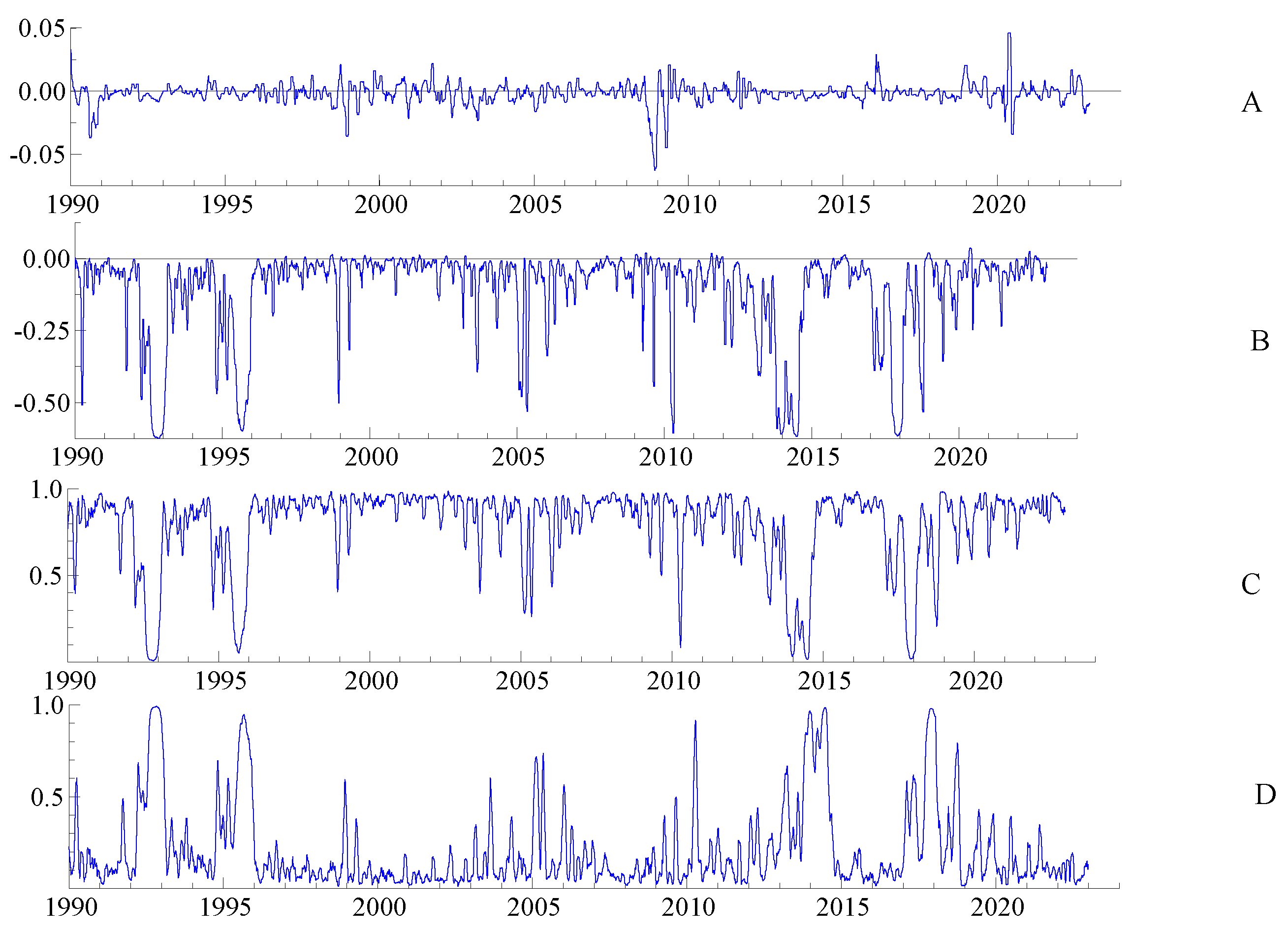
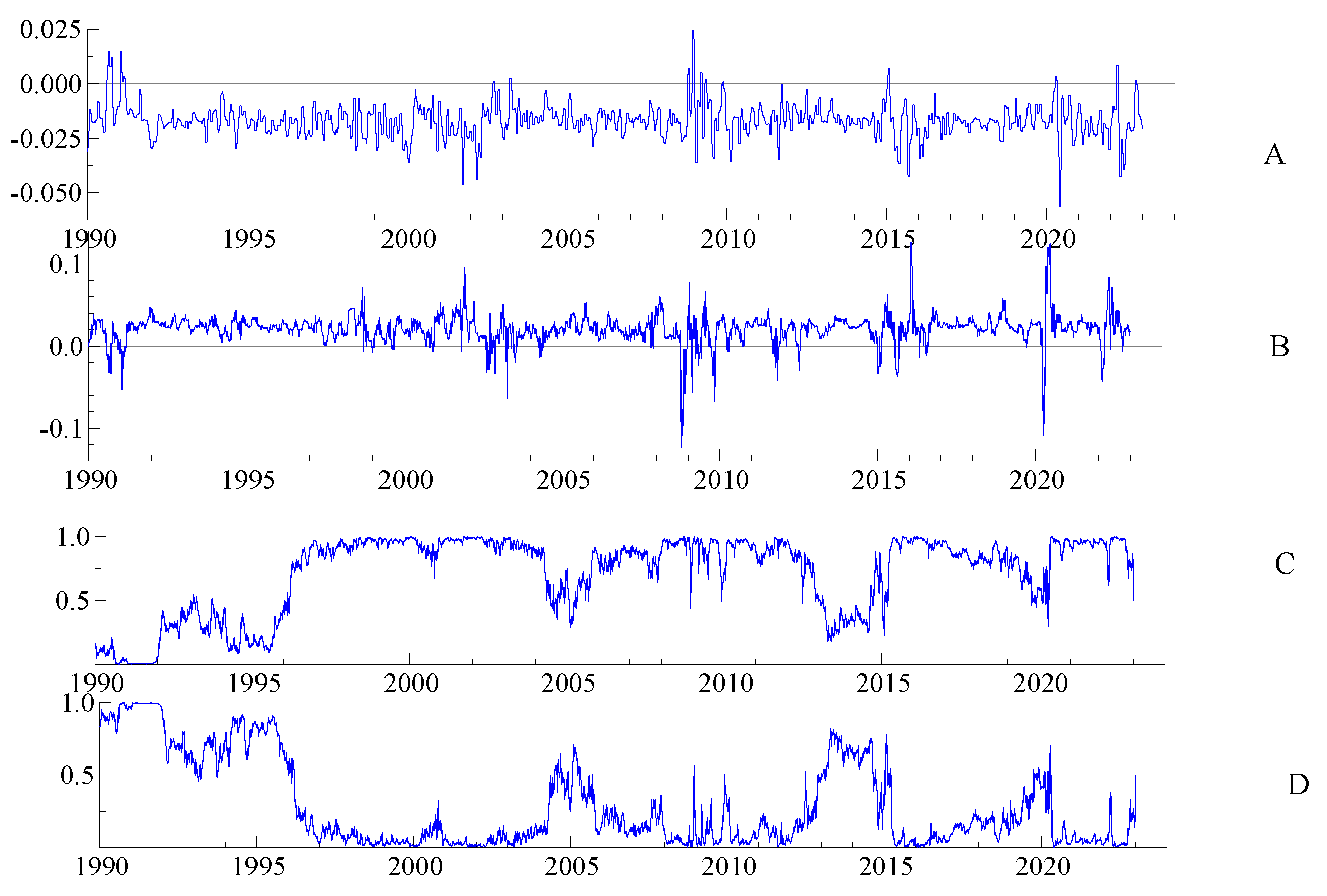
Figure 1, Figure 2, Figure 3 and Figure 4 show the dependence paths between the US/Europe stock and oil markets given by the dynamic copula model and the dynamic regime-switching copula model, as well as their filtering probabilities on their high and low regimes, to obtain a better picture of their time-varying evolution. The linear correlation coefficient is given by the Normal copula (Figure 3 and Figure 4) while the upper and lower tail dependencies are given by the SJC copula (Figure 1 and Figure 2).

Figure 3C,D and Figure 4C,D represent the estimated smoothing probabilities of being in the high/low dependence regime for the SP500–WTIoil and Eurostoxx50–WTIoil, respectively. It can be seen that both SP500 and Euro Stoxx50 volatilities produce regime-switching and time-varying dependence with WTI crude oil.

Overall, the time-varying correlation, given by the dynamic copula, between the stock and oil markets was weak (Figure 3A and Figure 4A). The dependence between the SP500 and WTI crude oil volatilities given by the RS model (Figure 3B) was low but with jumps related to a negative increase in correlation reaching $-0.5$ during the high dependence regime on specific dates (end 1991, mid 1995, 2009–2010, between 2014 and 2015, end 2017, end 2019). These shifts in dependence, joined by a change in the regime from low to high, can be attributed to different events: the Iraqi invasion of Kuwait in mid-1991 and the beginning of the Gulf War; the global financial crisis around 2008/2009; the oil price crash and plunge in 2014; and the COVID-19 pandemic).

Copula functions are a powerful tool for isolating and examining the dependency structure. We can link the sudden rise or fall of correlations to major economic, financial, and global events given their corresponding periods of time; however, a more thorough regression analysis with macroeconomic and financial indicators needs to be conducted to further confirm the results.

Notice that the time-varying correlation with and without regime switching between the European stock market and WTI oil (Figure 4A,B), although also low and weak, did not exhibit a distinguished regime shift with sudden jumps in the correlation like the SP500–WTI oil. Thus, we can say that there is a difference in the reaction of the European stock index and the US stock index to exogenous shocks and news. This means that the US stock market is more affected by instability, crises, and exogenous shocks than the European market, which is in accordance with Schuenemann et al. (2023).

The upper and lower tail correlations given by the dynamic copula and the regime-switching copula are given in Figure 1 and Figure 2. Two regimes, high and low, were detected depending on the dependence structure. The changes in the tail correlations given by the RS copulas were not as straightforward and distinct as their conditional linear correlations (Figure 1B and Figure 2B for lower tails, Figure 1D and Figure 2D for upper tails). Both copula models (with and without regimes) highlighted and confirmed the time variation and nonlinearity of the dependence in both the upper and lower tails. However, as expected, the RS copula was more fitted to represent the different regimes in the dependence structure. Apart from a brief peak in 1995, both upper and lower tail dependencies given by the RS SJC copula for both studied pairs were stable overall before the end of 2008 and increased slightly after, particularly for the SP500–WTIoil (up to 1.1 for the lower tail and up to 0.25 for the upper tail). In addition, the extreme dependency was higher in the lower tail than in the upper tail. However, for Eurostox50–WTIoil, tail dependencies were more stable and did not show a distinguished pattern with each regime (Figure 2B,D). Again, we show that the European stock market is less affected by instability and crises than the US stock market.

Therefore, for both pairs, we can confirm that their tail correlations increased during the global crisis. However, this increase was more important in the lower tail than in the upper tail. In other words, WTI crude oil prices and European and US stock markets were more dependent and linked when extreme negative events that occurred than with positive extreme events. They are more affected by bad news and losses that naturally induce a rise in their lower tail co-movements. However, this phenomenon is more visible and noticeable in the US stock market.

To sum up, the dependence of WTI oil with the SP500 and the EuroStoxx50 can be divided into two stages: a relatively calm state and a turbulent state.

The calm state corresponds to the low regime, where conditional correlations between the studied variables were weak or negative. This finding has been confirmed by other researchers (Cifarelli and Paladino (2010); Balcilar et al. (2015)). The turbulent state corresponds to the high regime during exogenous shocks, crises, news, or turmoil, where dependency increases significantly. In addition, with WTI crude oil, both the SP500 and Euro Stoxx 50 exhibited asymmetric tail correlations due to lower tail correlations being higher than upper tail correlations. However, it was much more noticeable in the US equity market than in the European one. In other words, the US stock market is more affected by exogenous shocks and instability than the European stock market, which is in accordance with Schuenemann et al. (2023).

This shift in dependence can be attributed to changes in the economy, the supply and demand fundamentals, Chevillon and Rifflart (2009), along with increasing trading activity by speculators and financial institutions in derivatives and financial markets (the financialization of commodities).

It is known that commodity investments present an attractive aspect for investors and financial institutions since they do not behave like traditional financial assets. Therefore, they tend to include them in their mixed-asset portfolios for diversification benefits to improve the risk-adjusted performance of their investments. However, the results of this paper suggest that during crises and turmoil, the energy market, particularly oil, cannot be a good hedge to protect investors from any potential losses related to their investments. In other words, oil cannot be considered a safe haven to help reduce portfolio risk. Investors should try another class of commodities instead of energy that follows a cyclical pattern and is affected mostly by economic fundamentals and demand and supply variations, and not by external factors such as crises, turbulence, and speculations. Our findings contradict some studies in the literature, such as Lamm (1999) and Chong and Miffre (2010), who found that commodities offer diversification benefits even in periods with high volatility.

6. Conclusions

In this paper, I study the dependence between the US and European equity markets represented by the SP500 and the Euro Stoxx 50 with the WTI oil price returns using the copula approach. Both the dynamic and the Markov copula models are used. The difference between the two is that the latter one, proposed by da Silva Filho et al. (2012), integrates a Markov chain in the intercept term of the equation, describing the time evolution dependency. It can provide a better understanding of the relationships between the studied variables than with only the dynamic conditional copula. After properly modeling the marginals of the returns using an ARIMA-GARCH/GAS model to extract their volatilities, we proceed to the estimation of the RS copula model. This step is not straightforward and is time consuming since we deal with an unobserved Markov process. For that, I used the Kim filter to obtain the smoothing probabilities and estimate the copula parameters.

The empirical results confirmed the time-varying and non-linear aspect of the dependence between the variables, alternating between high and low regimes. This can be explained by the phenomenon of the financialization of commodities, where, starting around 2003, there was a huge expansion of commodity transactions linked to investments. More and more investors and financial institutions used the commodity market for the purposes of asset management and portfolio allocation. Thus, commodities, or at least some of them, started to behave more like traditional financial assets. That is why they were also affected by the financial crisis in the same way as stock market assets.

The existence of two persistent regimes (high and low) in the dependence structure was proven by the dynamic RS copula model. In addition, the US market was more affected by economic and financial turmoil than the European market. The last point to mention is the asymmetry between both SP500 and Eurostoxx50 with the WTI oil. In fact, dependence in the lower tail was higher than the dependence in the upper tail for both pairs, meaning that extreme negative returns are more likely to be linked and tail-dependent in periods of economic turmoil and crisis (bear market), while extreme positive returns (bull market) are more tail-independent.

Possible directions for future research would be to include other exogenous variables, like some financial instruments and macroeconomic indicators, to study more in detail the relationship between the oil price and the stock market prices. Also, considering other energy commodities like natural gas, it would be interesting to see if there is any difference in their behavior compared to oil. In addition, a possible extension of the RS model in order to measure and evaluate more thoroughly the dependence structure is to introduce a hidden state in the autoregressive term of the dependence equation of the copula function, not just the constant term, and not limit the number of regimes to two.