1. Introduction
The workhorse in empirical modeling of economic time series is still constituted by the vector autoregressive (VAR) model. The VAR model explains the process
using the difference equation:
where
is a white noise process. Under the stability assumption
for
, this equation has a unique stationary solution. Often, prior to VAR modeling, deterministic components are extracted such as a constant, a linear trend, and seasonal dummies.
Oftentimes, this model is seen as an approximation to the data-generating process. This happens, for instance, if the data are generated by a vector autoregressive moving average (VARMA) process, where
for white noise
with expectation zero and variance
. The VARMA system
(where the pair
is left-coprime) is called invertible if
. Under stability and invertibility, we obtain the VAR
representation
Under invertibility, we have
where
typically is the smallest modulus of the solutions of
. Thus, the coefficients converge to zero, geometrically implying that a VAR approximation seems plausible.
When estimating a VAR model, one has to decide on the lag length,
h. This choice of the lag length is typically based on adding a penalty term to the estimation accuracy as measured using the residual variance
for a range of potential lag lengths
, resulting in so-called
information criteria. Here, the residual variance
is estimated from data as follows:
1
If no structural restrictions apply, the matrices
are typically estimated using OLS or the Yule–Walker equations (see, for example,
Hannan and Deistler 1988, p. 211).
2 In this paper, we only consider OLS estimation.
Information criteria then are defined as
Here,
denotes the number of parameters estimated in the conditional mean equation, and
is a penalty factor. The most prominent choices are
AIC (
) and
BIC (
). The minimal integer
minimizing IC is then the selected lag length.
3For the case of stationary invertible VARMA processes, the asymptotic properties are well documented in section 6.6 of HD. Under appropriate assumptions on the noise (see Theorem 6.6.3 of HD) and upper bounds
for the lag length, for
estimated using
BIC, we have
a.s. (Theorem 6.6.3 of HD), and the same limit holds for
in probability (Theorem 6.6.4 of HD), where
. Consequently,
. Thus, in this case, asymptotically, the approximation error (
2) is of the order
.
Moreover, Theorem 7.4.7 of HD states that in a more general setting, if
is not generated by a finite autoregression under the same assumptions on
, as above and where
, we have
uniformly in
, if
. Here,
is independent of
h. Now impose the following assumption on the sequence
:
Assumption 1. For the sequence there exists a twice continuously differentiable function with second derivative such that and Under this assumption HD show that the optimal h (for ) is close to a minimizer of the deterministic function .
The limitation to stationary processes and autoregressive coefficients
declining fast enough excludes persistent processes such as unit root processes that are often encountered in economic time series. It is common practice, nevertheless, to select the lag length using information criteria also in case of highly persistent processes. For integrated processes of the I(1) kind, this is backed by some results in the literature, such as
Ng and Perron (
1995), stating that lag length selection for VARMA models has properties analogous to the stationary case. These results are generalized to a larger class of processes in
Lütkepohl and Saikkonen (
1999).
4However, in the literature, there are currently no results available for the I(2) case of doubly integrated processes. This class of processes was introduced by
Granger and Lee (
1989), who illustrated the main underlying idea using an example from inventory processes: if the demand for a product (a flow variable) is modeled as an I(1) process (which is realistic in a number of cases; see
Granger and Lee 1989), then the stock of the product at the producers will be I(2), as stock variables sum up the corresponding flow variables. In a macroeconomic framework, I(2) processes have been investigated, for example, by Johansen and Juselius and coworkers, who argue that I(2) processes play a role if the model contains nominal quantities, as inflation often is found to be integrated. Since inflation is the change rate of prices, it follows that prices must be I(2) then (see, for example,
Juselius 2006, chps. 16–18, or
Johansen 1995, chp. 9).
While these models have been used in the literature, the corresponding inferential methodology focuses on the case of autoregressions with a finite lag length. If the data-generating process is more general, such models are often an approximation and must involve the selection of the lag length. In practice, this is performed using information criteria such as AIC or BIC also in this situation while a theoretical justification is missing.
This paper closes the following gap: we provide a general result for the asymptotic behavior of lag length selection using information criteria for I(2) processes, linking the performance for the I(2) processes to a related stationary process for which the results of HD can be applied. The proof of this result can be found in the appendix. The result is illustrated using a simulation study in
Section 3.
2. Integrated Processes
The key to the results for integrated processes is the insight that the OLS residuals of (
1) and—for example—of the vector error correction equation
are identical. Since the information criteria are a function of
(see (
3)), they are invariant to linear transformations of the regressors as well as to transformations of the dependent variable by adding linear functions of the regressors.
If in (
6)
, this defines a VAR(
) process
for which stationary theory applies under stability assumptions for
. As in this case the estimation of
is superconsistent, one would suspect that the inclusion of
as a regressor does not change the lag length selection substantially except for adding one lag to account for the differencing. A similar reasoning applies in the case of reduced rank of
.
Paulsen (
1984) shows that for finite-order autoregressive I(1) processes, indeed, the results for the stationary case can be extended.
Lütkepohl and Saikkonen (
1999) extend some of the results to VAR(
∞) I(1) processes, rectifying earlier incorrect proofs in the literature.
Bauer and Wagner (
2004) provide theory for the case of multifrequency I(1) processes such as seasonally integrated processes by using the vector of seasons representation linking the multifrequency I(1) case to the I(1) case.
In more detail, let, in the I(1) case,
, where
and
5,
denote matrices such that
is orthonormal. Let
. Then assume that
where
and where it is assumed that
. Under these assumptions, it follows that we obtain the VAR(
∞) representation
where
, implying the VAR(
∞) representation
for the I(1) process
. Furthermore, the triangular representation (
7) implies that the process
is integrated and not cointegrated; compare, for example,
Saikkonen and Lütkepohl (
1996), sct. 2.
The corresponding VAR(
h) approximation is given as
. Premultiplying with
and using that (for
), the set of regressors
(of dimension
) can be linearly transformed into the set of regressors
(of dimension
) plus
, we obtain (for appropriate coefficient matrices)
where
. Using (
7) then leads to
Here, all variables are stationary except for
, which is I(1) and not cointegrated by design. Consequently,
has to hold (compare equation (A.2) in
Saikkonen and Lütkepohl 1996). Omitting this regressor, the approximation almost equals a VAR(
h) approximation of
except for the inclusion of
instead of the full vector
. We have
for each
where
denotes the residual variance in a VAR(
h) approximation for
. This shows that the residual variance of
and the one of
are closely related.
Thus, the essential step in linking the asymptotic properties of the lag length selection in the I(1) case (obtained from inclusion of ) to the ones in the stationary case (assuming that is left out, which is infeasible in practice as the matrix is not known prior to estimation) lies in establishing that the inclusion of has negligible effects.
For the I(2) case, the same route can be taken. To this end, consider processes according to the following assumptions:
Assumption 2. Let be an I(2) process (not generated by a finite-order autoregression) obtained as a solution to the equation (with deterministic values , and )where are full column rank matrices;
The function (converging absolutely for ) fulfills that implies that or ;
With (where are of full column rank ) the matrixis nonsingular.
Furthermore, the process is independent identically distributed (iid) with mean zero, variance , and with .
From these assumptions, it follows that the process
is I(2) with cointegration and potentially multi-cointegration occurring. The structure of the process is best seen in the triangular representation of the process, which is equivalent to the one used above (see, for example,
Li and Bauer 2020): assume that the stationary process
is generated according to
(for suitable assumptions on
including
) and related to the process
via
where
, and
are as in Assumption 2. Then, clearly,
is I(2) and not cointegrated,
is I(1) and not cointegrated, and
is I(1) and cointegrates with
to stationarity for nonzero
A. If
, it is stationary.
6 The cointegrating relations
between an I(1) and a differenced I(2) process are termed
multi-cointegration by
Granger and Lee (
1989).
It follows that (using
)
Denoting
and using
, we obtain from premultiplying the above equation with
:
Noting that
such that
, it follows that
and thus
This confirms the low rank decompositions
and
as well as the rank of these matrices. The VAR(
∞) representation then follows from calculating the coefficients of
and
. Therefore, the triangular representation immediately shows that the process
is I(2) and not integrated of higher order, but leaves the dynamics contained in
unspecified. The VAR(
∞) representation, on the other hand, focuses on the dynamics, but makes the derivation of the properties of the processes defined by the difference equation less immediate.
To illustrate the function of the constraint (
8) to exclude higher order of integration in the solutions process, assume for the moment that the process
is I(2) and consider
:
Here,
(as
denotes the second block row of
) such that
. Now, using the first difference of the model equation, we see that
such that
for some stationary process
.
Combining these facts, we see that
for some matrix
. Thus (the last equation defines
),
Consequently,
The right hand side process is a stationary process with nonsingular spectrum at
as it equals
for stationary process
. This shows that for the properties of
, the square matrix
is of major importance: if it is nonsingular, then
is stationary. If it is singular such that the process still contains a unit root, then
is an integrated process. Hence, the nonsingularity of (
8) ascertains that the solution process
is I(2) and not I(3) (or integrated of even higher order).
For simplicity of presentation, no deterministic terms are included in the model formulation. Then, the corresponding result for I(2) processes is the main result of this note:
Theorem 1. Let be generated according to Assumption 2. Let the lag length selection be performed by minimizing the information criterion with penalty term over the integers . Let the minimal minimizing argument be denoted as . Then,
- (i)
for each constant .
- (ii)
If Assumption A1 holds for with function , then in probability, where minimizes the function .
- (iii)
If is an I(2) invertible VARMA process corresponding to the left-coprime pair , then in probability, where .
The same results hold if the process is demeaned and/or detrended before estimation.
The result shows that the lag length selection essentially follows the minima of the function analogously to the stationary case. In the VARMA situation, we obtain a lag length that is proportional to and depends on the location of the zero closest to the unit circle. Otherwise, the minima of will increase for increasing sample size as the penalty term tends to zero for while decreases monotonously.
The assumptions here are stronger than needed in almost all aspects. Convergence of
on
can be weakened to
for suitable
. In addition, the iid assumption for
can be weakened to martingale difference type assumptions as in HD. I here use the stronger assumptions in order to stay in line with
Li and Bauer (
2020) (in the following LB) on which the proof (to be found in
Appendix A) is based.
7Note that Assumption 2 excludes the finite lag length case in which is generated by an autoregression of, say, order . In this case, we have . It follows that, asymptotically, with probability one if . Furthermore, the probability of tends to zero for as a function of T as the penalty then dominates the estimation error for . This demonstrates that BIC is (weakly) consistent for VAR() processes.
Inspecting the proof, it is obvious that analogous results also hold for the I(1) and the multifrequency I(1) case. Moreover, often, not only is the lag length selected uniformly for all component processes, but different lag lengths are selected for each component. In addition, in this case, the proof in the appendix can be adapted to show that the asymptotic properties in the integrated case are analogous to the ones in the stationary case obtained by suitably differencing the process.
Such an extension also pertains to VARX models. In this situation, it is also possible to be more general such that the exogenous process does not need to possess a VAR(∞) representation with sufficiently fast decreasing coefficients, but may show (stationary or integrated) long memory if the number of lags to be included is subject to an upper bound. The bottom line in all such cases is that the integration properties of the process are of less concern, if differencing leads to stationarity with sufficiently fast decaying impulse responses.
Finally, note that similar results appear possible for processes of higher order of integration.
3. Simulations
In this section, the theory is illustrated with a simulation exercise involving MA(1) processes of the form:
for standard Gaussian white noise process
. These processes are stationary and invertible for
being a stable matrix. In the scalar case, the smallest zero of the process equals
. Therefore, the required number of lags in an autoregressive approximation is controlled via
and is expected to grow similar to
as a function of the sample size.
A total of realizations of the process with sample size , and are simulated, and one parameter is varied on a regular grid.
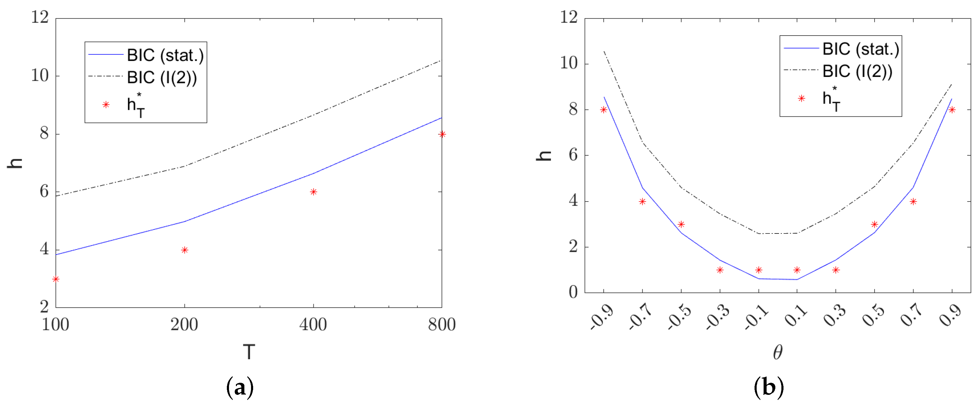
We thus investigate the increase of the average selected lag length for univariate MA(1) processes as a function of the sample size as well as the location of the zero closest to the unit circle. This is performed for the stationary process as well as for a doubly integrated MA(1) process obtained via double summation of the stationary process. The double integration is expected to add two lags compared to the lag length required for the stationary process as . Furthermore, the double integration potentially also adds a deterministic quadratic trend. Thus, lag length selection is performed on the corresponding detrended process in the I(2) case.
Figure 1 shows the resulting average lag lengths selected using
BIC. The main effects contained in the theorem are clearly visible: the selected lag length increases with sample size. The logarithmic scale on the x-axis for plot (a) shows
8 the roughly linear increase in
. In addition, larger absolute values of
result in larger lag lengths. The average selected lag lengths with
BIC are very similar to the optimal values
(corresponding to the stationary process
). The doubly integrated processes
require roughly two more lags in all cases compared to the stationary process
except close to
(which is close to a pole zero cancellation), where only one additional lag results in the lag length selection on average.


