Abstract
Health preference research (HPR) is the subfield of health economics dedicated to understanding the value of health and health-related objects using observational or experimental methods. In a discrete choice experiment (DCE), the utility of objects in a choice set may differ systematically between persons due to interpersonal heterogeneity (e.g., brand-name medication, generic medication, no medication). To allow for interpersonal heterogeneity, choice probabilities may be described using logit functions with fixed individual-specific parameters. However, in practice, a study team may ignore heterogeneity in health preferences and estimate a conditional logit (CL) model. In this simulation study, we examine the effects of omitted variance and correlations (i.e., omitted heterogeneity) in logit parameters on the estimation of the coefficients, willingness to pay (WTP), and choice predictions. The simulated DCE results show that CL estimates may have been biased depending on the structure of the heterogeneity that we used in the data generation process. We also found that these biases in the coefficients led to a substantial difference in the true and estimated WTP (i.e., up to 20%). We further found that CL and true choice probabilities were similar to each other (i.e., difference was less than 0.08) regardless of the underlying structure. The results imply that, under preference heterogeneity, CL estimates may differ from their true means, and these differences can have substantive effects on the WTP estimates. More specifically, CL WTP estimates may be underestimated due to interpersonal heterogeneity, and a failure to recognize this bias in HPR indirectly underestimates the value of treatment, substantially reducing quality of care. These findings have important implications in health economics because CL remains widely used in practice.
1. Introduction
Given their knowledge of healthcare and available resources, patients, clinicians, payers, the industry, and policymakers all seek to create the best structures, processes, and outcomes (Donabedian 1988). Each decision maker aims at maximizing the benefits while minimizing the risks and cost. Healthcare systems are facing a paradigm shift towards value-based healthcare (Porter and Teisberg 2006). Health preference research (HPR) is the subfield of health economics dedicated to understanding the value of health and health-related objects using observational or experimental methods. Understanding the value of health and healthcare can inform decisions at many different levels of healthcare decision making. These include basic drug discovery and clinical trials, patient-level care, and policymaking for the community by a range of stakeholders and decision makers (Rubio et al. 2010).
By definition, the theoretical framework underlying HPR rests on two constructs: “health” and “preference.” Health, according to the World Health Organization (1946), is “a state of complete physical, mental and social well-being and not merely the absence of disease or infirmity”. Like any construct, one person’s definition of “health” may differ from another’s, and as such, it is always measured with a degree of error; describing it also requires a broad array of indicators. Preference requires a comparison and may be defined as “a greater liking for one alternative over another” (Simpson and Weiner 1989). Health preference researchers typically assume that people prefer better and/or more health to worse and/or less health, and behave accordingly when they make health-related decisions. To understand the value of health and healthcare, a researcher examines choices by patients, clinicians, payers, policymakers, or anyone engaged in health-related decisions.
In HPR, health and preference are linked together through choices—the unit of observation in a health preference study. Formally, choice refers the selection of an object from among two or more alternatives. When we observe an individual’s choices, this behavior implicitly reveals their ordering of alternatives or objects (White 1969). Researchers typically assume that each choice between health-related alternatives maximizes decisional utility (Luce 1959; Marschak 1960). Health preference studies use observational and experimental methods to collect empirical evidence on health-related choices.
A discrete choice experiment (DCE) is a behavioral study where respondents are allocated a series of choice sets under a hypothetical situation. In each task, the respondent is asked to choose among two or more alternatives in each choice set. As part of the DCE protocol, their choices are observed, captured, recorded, and analyzed as a means to test one or more hypothesized causal relationships. Often, alternatives are described using a descriptive system of multilevel attributes, and the choice sets may include a referent alternative (e.g., opt-out). In health economics, the primary purpose of a DCE is to test and estimate the causal relationships between attribute levels and preferential choice behaviors. However, in DCEs conducted in other fields, such as audiology, the primary purpose of DCE is to assess the effects of a stimulus on perceptions. Apart from causal relationships, health economists conduct DCE to examine the willingness to pay for alternatives or predict choice behaviors under hypothetical situations (e.g., health technology assessment).
Between DCE respondents, the effects of attributes on behavior may vary (i.e., interpersonal heterogeneity) due to differences in individual utilities. Such differences in utilities between persons may be stochastic or systematically associated with observable or unobservable factors. Observable heterogeneity refers to observed (by the researcher) factors (e.g., age) that are associated with observed effects (also known as explained heterogeneity). On the other hand, unobservable heterogeneity refers to latent factors associated with the unobserved effects (e.g., risk perception). Multiple researchers stated that a failure to account for heterogeneity may lead to egregious differences between the estimated and true values in a choice analysis (Bhat 1998; Brownstone and Train 1999; Chamberlain 1980; McFadden and Train 2000). However, the extent of such differences is unclear.
Like in panel data analysis more generally, there are two general approaches to account for interpersonal heterogeneity depending on the experimental design. In some cases, the DCE has a large number of tasks per respondent relative to the number of parameters; therefore, the analyst can estimate individual-specific parameters per respondent (namely, fixed effects). When this is not the case, interpersonal heterogeneity is unobservable; nevertheless, the analyst may estimate a random parameter model by making distributional assumptions about the prevalence of parameters within the population (e.g., mixed logit). In this simulation study, we examine the implications of ignoring interpersonal heterogeneity. We simulated a standard DCE under various forms of unobservable interpersonal heterogeneity and assessed the implications of ignoring this heterogeneity. More specifically, we generated trinomial responses for a standard DCE with a full factorial design and individual-specific coefficients varying over individuals. However, we ignored heterogeneity and estimated the conditional logit (CL) model to examine the differences between the estimated and true coefficients.
This paper shows what happens when different types of heterogeneity are ignored, and the implications for health economics, where conditional logit remains to be a standard modeling approach. By comparing the results with the true values, this paper clarifies whether ignoring certain types of heterogeneity alters the interpretation of willingness-to-pay (WTP) and choice predictions. For simplicity, the results of this study are limited to just one DCE and may lead other researchers to identify similar patterns under different experimental designs or types of heterogeneity (e.g., latent classes).
1.1. Types of Unobservable Heterogeneity
In HPR, unobservable interpersonal heterogeneity may be classified as either informative or uninformative. Uninformative heterogeneity implies that parameters differ between persons, but knowing one parameter of a person does not inform about the person’s distribution of another parameter (i.e., uncorrelated parameters). Under this form of uninformative heterogeneity, individual-specific parameters vary between persons, but these parameters are not correlated. Conversely, informative heterogeneity implies that the individual-specific parameters are correlated through latent factors.
Furthermore, informative heterogeneity may be separated into two subtypes on the basis of which parameters are correlated. Substitution patterns (e.g., Brownstone and Train 1999) refer to the presence of a latent factor that causes an association with alternative-specific constants (ASCs). For example, the classical red-bus–blue-bus problem refers to a positive correlation between the two bus alternatives, where a red bus is a substitute for a blue one (e.g., Quandt 1970). An ASC is not the same as a nominal attribute. In this classical problem, every set includes three fixed alternatives, namely, a car, a red bus, and a blue bus. If the color and mode were nominal attributes and varied independently, some sets might include three buses. In health economics, a more common example is a choice set with multiple fixed treatment options (e.g., a brand-name medication and a generic medication) and “watchful waiting” (i.e., no medication).
Taste patterns (e.g., Revelt and Train 1998) refer to the presence of a latent factor that causes an association between attribute coefficients more generally (i.e., attribute importance). In health economics, each alternative may vary by out-of-pocket price, wait times, and other attributes. The coefficients of these attributes may be correlated. For example, individuals who are willing to pay more for their healthcare may also prefer more luxurious services (e.g., a brand-name medication when a generic medication is available).
Imagine a specific alternative (e.g., a brand-name medication). Under uninformative interpersonal heterogeneity, the effect of a specific brand varies between persons, but this effect is not associated with another alternative’s effect (i.e., substitution pattern) or the effects of any attributes (i.e., taste pattern). Alternatively, latent factors may induce informative heterogeneity, such as a substitution pattern between brands or a taste pattern between a brand and out-of-pocket cost.
For simplicity, we generated preferential choice behaviors for a standard DCE with a full factorial design (Appendix A) and individual-specific unobserved coefficients drawn from a normal distribution. Each task represents a choice among three alternatives to illustrate uninformative and informative heterogeneity, including substitution and taste patterns. Each alternative is described using a nominal and a numeric attribute, namely, medication and out-of-pocket price. For example, the correlation between the effects of brand and generic is a substitution pattern, and the correlation between the effects of medication and price is a taste pattern. Willingness to pay for a brand-name medication is the ratio of the brand-name medication and price effects. This DCE was constructed to mimic the classic red-bus–blue-bus example.
1.2. Choice Modeling with Unobservable Heterogeneity
Historically, econometricians estimated the parameters of CL models under the assumption of homogeneity. When heterogeneity is absent, the identification of the CL is standard and its nuances are beyond the scope of this paper. Choice probabilities of the CL model have a closed-form which can be evaluated analytically using the maximum likelihood (ML) estimator. When heterogeneity is present and observable, the CL model can be adapted to “explain” this heterogeneity, and its ML estimation is again computationally simple. However, one of the drawbacks of the CL model is that it does not account for unobservable heterogeneity. Failing to account for unobservable heterogeneity (i.e., uninformative and informative) may lead to misleading statements about the WTP and choice predictions (Bhat 1998; Brownstone and Train 1999; Chamberlain 1980; McFadden and Train 2000). There are more flexible models that allow for unobservable heterogeneity, such as mixed logit specifications; however, our main purpose is to understand consequences of ignoring unobservable heterogeneity.
For this simulation study, we explore the differences between CL estimates and the mean of their true values depending on the type of unobservable heterogeneity. For the purposes of this paper, we define bias as the difference between the estimates of the CL under ML and the mean of the true values used to generate the responses. First, we examine the case of omitted variance bias where one or more parameters vary, but are uncorrelated. Understanding such uninformative heterogeneity is a necessary precursor to the examination of informative heterogeneity (i.e., correlations). Second, we examine the three cases of omitted correlation bias: substitution patterns, taste patterns, and both.
There are more flexible models of DCE responses, such as mixed logit specifications, which allow for unobservable heterogeneity. However, our main purpose is to understand consequences of ignoring unobservable heterogeneity. Furthermore, Clark et al. (2014) reported that, in health economics, 44% of DCE studies during 2009–2012 used the CL (or multinomial logit) model, while 21% used the mixed logit model during the same period. Our findings have intriguing implications for the majority of health preference studies, including benefit–risk analyses and health valuations.
2. Methods
2.1. Model
The theoretical framework of this choice analysis is based on random utility maximization (RUM) theory (Marschak 1960). According to RUM theory, utility function of individual for alternative at choice situation can be decomposed into a deterministic part of utility (representative utility) which is observed by the researcher, and a random part of utility that is not observed by the researcher. Following McFadden (1974), individual i chooses an alternative j if and only if the probability that utility associated with alternative j is higher than that of utilities associated with all other alternatives:
Choice probabilities are calculated on the basis of a relative measure where utility of one of the alternatives in the choice set is taken as a reference. To derive the choice probabilities, distributional assumptions are needed about the random part of utility. The CL model is derived under the assumption that is independently and identically distributed (IID) with extreme value type I (EV1) distribution (e.g., Brownstone and Train 1999; McFadden and Train 2000; Revelt and Train 1998; Train 2009). As a result, the difference between two IID EV1 random error terms () has logistic distribution. This implies that the choice probabilities of the CL model can be expressed in terms of logistic distribution with cumulative distribution function:
In this simulation study, we generated choices among three alternatives, where the third alternative served as a referent (i.e., opt-out) (e.g., Campbell and Erdem 2019). For example, imagine the decision on whether to take a heartburn medication: brand-name, generic, or no medication. Hence, we assumed that the representative utilities of the three alternatives took the following form:
Therefore, utility differences take the following form:
where and are out-of-pocket prices (see Appendix A for the out-of-pocket price), and are alternative-specific constants (ASCs) for each respondent, is an individual-specific price coefficient, and are two utility differences, and finally, and are differences in IID EV1 error terms. Under this specification, the willingness to pay for each medication is the ratio of the ASC and price coefficient, .
In our model specification, we used two ASCs ( and ) to allow their correlation. Alternatively, a nominal attribute for opt-in () may be included instead of two ASCs. However, that specification would deviate from the red-bus–blue-bus example. Similar in health economics is the case of choosing among three ways to see heartburn relief, where the alternatives are a brand-name medication, a generic medication, or doing nothing. It seems appropriate to allow the ASCs for the brand-name and generic medications to be correlated and not combined as a treatment attribute.
To incorporate interpersonal heterogeneity, we express the prevalence of individual-specific ASCs and within the population using a multivariate normal distribution with . Covariance matrix is
where , , , , and . Uninformative heterogeneity occurs when correlation parameters are restricted to be equal to zero , in which case, covariance matrix is diagonal. On the other hand, informative heterogeneity allows for the correlation of individual-specific parameters, such that .
2.2. Simulation
In the data generation process, the true means of the representative utility parameters (Equation (3)) were fixed at and (i.e., brand-name, generic, and out-of-pocket price, respectively). The out-of-pocket price values that we used in this study ( and ) are presented in Appendix A. Furthermore, we generated various covariance matrices (Equation (5)) on the basis of the true values that we chose for the variances and correlations, and we refer to each distinct covariance matrix as a “parameter set” (see Table 1).

Table 1.
Parameter sets for informative and uninformative heterogeneity.
The simulated covariance matrices fall into six groups: the first three groups represent uninformative heterogeneity (i.e., uncorrelated parameters; ), and the last three groups represent informative heterogeneity (correlated parameters; ) where the variances were fixed at 0.15 for identification. For instance, in Group 2, we assumed that and ranged from 0.025 to 0.25 with increments of 0.025 (i.e., or ), and we assumed that . Since there were 10 different values for each and , we could create 100 combinations of parameter sets for the true covariance matrix. The rest of Table 1 can be interpreted in a similar fashion.
Across all simulations, the ratio of the mean (i.e., ) brand-name medication and price parameters was −1. Under homogeneity, this ratio represents WTP. Under heterogeneity, WTP is the mean of the true ratios (i.e., ), and its value depends on the correlation . In Group 4, the true mean WTP for the brand-name medication (A) monotonically decreased from −1.011 to −1.337 as the correlation increased from −0.95 to 0.95. This association is intuitive: a large negative correlation implies that the variations in and counterbalance each other (i.e., when is less than −1, and is more likely to be greater than 1). Likewise, a positive correlation implies that larger are more likely divided by a smaller , causing the mean WTP to be lower (i.e., <−1). Even in the absence of correlation, the mean WTP was around −1.2. By construction, CL is unable to estimate both mean parameters and willingness-to-pay consistently under interpersonal heterogeneity; however, the extent of the bias is unclear.
At first glance, Group 6 seems to contain 4000 combinations of parameters, since there are 10 different values of , and 20 different values of and (10 × 20 × 20); however, we eliminated parametric combinations that did not lead to a positive definite covariance matrix , reducing the number of sets to 2520.
For each parameter set, we simulated 1000 DCE datasets (), each including 25 choices () for 200 respondents () given a full factorial experimental design (see Appendix A). This design may include dominated alternatives. However, since this is a simulation study, the existence of dominated alternatives should not be a concern. With each simulated dataset, we estimated a CL model by ML, and compared the estimated and mean true parameters (, and ). In addition, we calculated the two WTP on the basis of the ratio of estimated parameters and predicted the 75 choice probabilities in the experimental design (3 alternatives by 25 choice set). We compared the true and estimated choice predictions (P) across the 1000 simulated datasets using Lin’s concordance correlation coefficient, which we denote as Lin’s (Supplementary Materials). Furthermore, we calculated the worst-case scenario in the results across all simulations on the basis of the ratio of estimated and true odds (Supplementary Materials).
3. Results
On the basis of 1000 simulations for each parameter set, Table 2 and Table 3 show the mean CL parameter estimates (and standard errors), and WTP under the Group 1 and 4 simulations. The remaining simulation results are included in the Supplementary Materials for reference.

Table 2.
Uninformative heterogeneity Groups 1a and 1b: no correlations.

Table 3.
Informative heterogeneity Group 4 results: taste patterns.
3.1. Uninformative Heterogeneity
The Group 1 simulation results (Table 2) exemplify the omitted variance bias under uninformative heterogeneity, with three noteworthy observations. First, for all values of and for , the estimated parameters of the representative utility differed from their true values by more than 3 standard errors; therefore, the null hypothesis and may be rejected under uninformative heterogeneity. Second, the difference between the true and mean estimates decreased when we increased the variance, suggesting that more uninformative heterogeneity can cause the estimated parameters to converge toward the true values. Lastly, the omitted variance bias was less than 0.07 in WTP. In other words, even though there may have been a significant difference in the CL estimates , and (i.e., omitted variance bias), the estimated WTP were close to their true values.
An increase in variation helps (to a certain level) in estimating the parameters more accurately. However, we cannot infinitely increase the true variances to decrease biases in estimated coefficients in order to achieve a point where the estimated coefficients are within 3 standard errors from their true values. However, from our experience, the most important factor that reduced biases in the coefficients occurred when we allowed variation in the cost coefficient (i.e., ).
3.2. Informative Heterogeneity
The Group 4 simulation results (Table 3) exemplify the omitted correlation and omitted variance biases under informative heterogeneity where but (taste patterns). For example, persons who prefer the brand-name medication may have a greater (or lesser) willingness to pay. Unlike Group 1 (Table 2), the CL estimates in Group 4 were close to their true values (i.e., within three standard errors). In fact, in all 38 different parameter sets of Group 4, the estimated , and were within 3 standard errors from their true values. Therefore, the null hypothesis and may not be rejected under informative heterogeneity.
Furthermore, we present the true and estimated WTP (i.e., T. WTP and E. WTP) for and . As the correlation decreased (increased), the estimated WTP for the () approach within three standard deviations of −1 was representing the ratio of the means (i.e., ) but misrepresenting the mean WTP (i.e., ). The results show a weak association between the CL WTP estimates and the correlation .
Table 4 demonstrates the implication ignoring substitution patterns in the classical red-bus–blue-bus example. For example, persons who prefer the brand-name medication may also accept the generic one because they lack an alternative (i.e., disfavor opt-out). Similar to the results in Table 3, the estimated WTP and consistently represented the ratio of means. However, they failed to accurately represent the true WTP.

Table 4.
Informative heterogeneity Group 5 results: substitution patterns.
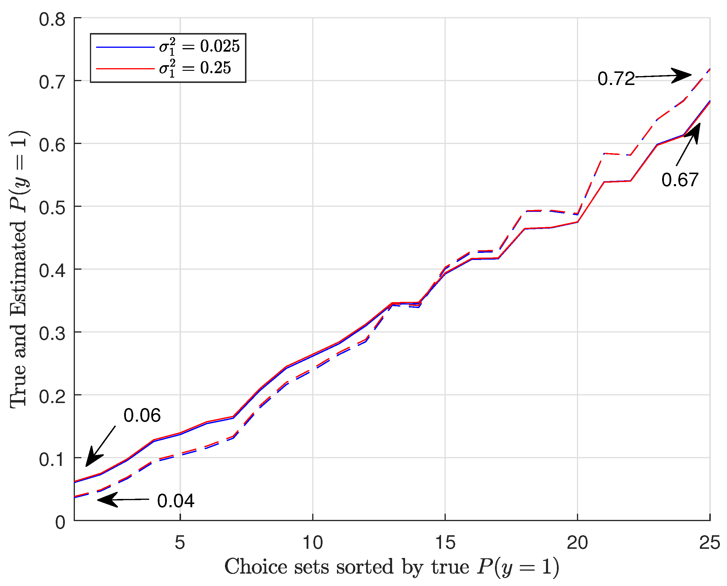
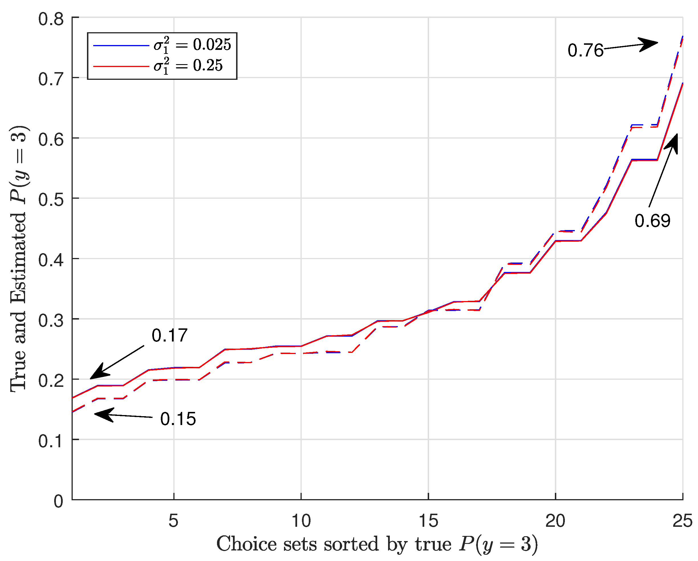
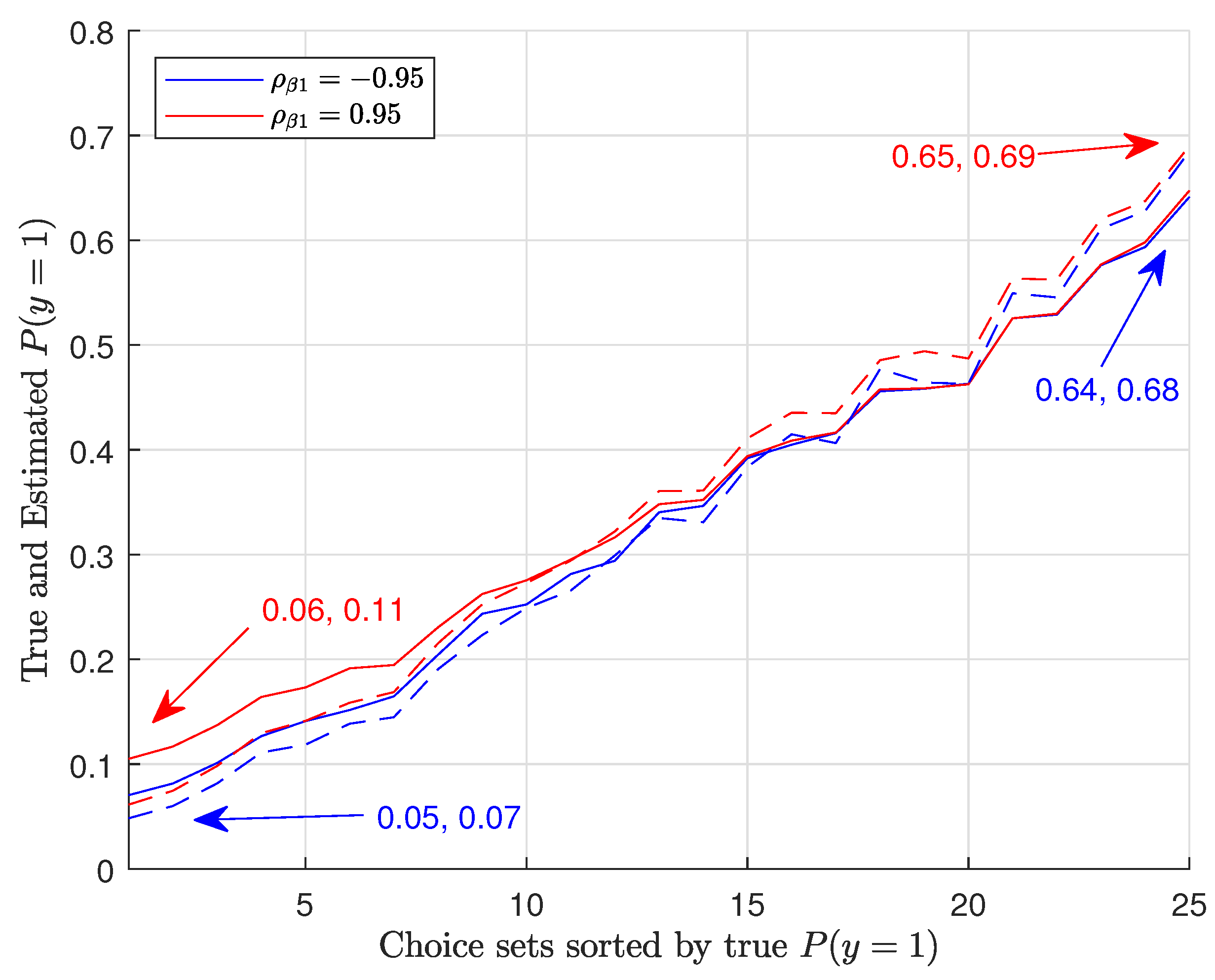
To better illustrate the effects of interpersonal heterogeneity on CL results, we illustrate the relationship between the true and estimated choice probabilities. Figure 1 shows the true versus estimated P(y = 1) for Group 1a in 25 choice situations for two different variances, . Similarly, Figure 2 shows the true and estimated P(y = 3) for Group 1a. In Figure 3, we plot the true and estimated P(y = 1) for Group 4 against 25 choice situations for two different correlations , and Figure 4 plots the true and estimated P(y = 3) for Group 4. The true choice probabilities are represented with straight lines and the estimated choice probabilities are represented with dashed lines. As you can see, in all of these figures, the estimated choice probabilities are close to the true choice probabilities irrespective of the variance parameter or correlation parameters .

Figure 1.
Plots of true and estimated P(y = 1) for Group 1a.
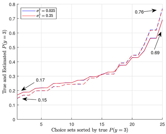
Figure 2.
Plots of true and estimated P(y = 3) for Group 1a.
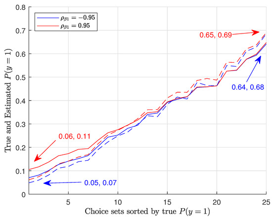
Figure 3.
Plots of true and estimated P(y = 1) for Group 4.
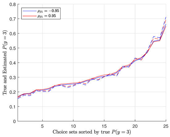
Figure 4.
Plots of true and estimated P(y = 3) for Group 4.
4. Discussion
These simulation results exemplify key implications of ignoring interpersonal heterogeneity in DCE, namely, the omitted variance and correlation biases. The results support the belief that assuming homogeneity in the presence of heterogeneity produces inconsistent results (see Chamberlain 1980). Specifically, the CL parameter estimates (, and ) differed from their true values under certain specifications of the data generation process. Likewise, we found substantive differences between the CL and true mean WTP. For instance, Table 3 shows a 20% reduction in WTP (i.e., [1.337 − 1.069]/1.337 = 0.2). Interpersonal heterogeneity generally implies that the CL enlarges the parameter estimates and increases the WTP estimates (i.e., less negative). Nevertheless, these differences largely factor out in the choice probabilities.
Within health economics, the findings support the conclusion that CL WTP estimates for medical treatments may be underestimated due to interpersonal heterogeneity. Furthermore, the assumption of preference homogeneity among patients (i.e., “misalignment with a patient’s wishes”) may contribute to an underestimation of the value of treatment, substantially reducing quality of care (Clapp et al. 2022). If the analyst conducted the DCE to solely predict choices in aggregate, the presence of interpersonal heterogeneity may not be as relevant. CL choice probabilities were similar to the true ones. The reason why the biases in the estimated coefficients did not transfer to the choice probabilities may have been because the influences of the interpersonal heterogeneity on the likelihood of choices reduce significantly when we pass the effects through the logit cumulative distribution function.
Although we characterized the estimated ratio as WTP (i.e., the ratio of the mean brand-name medication and price parameters), many health preference studies estimate similar ratios for other purposes. In a benefit–cost analysis, results are often expressed as the maximal acceptable risk (i.e., the ratio of the mean benefit and risk parameters) (Reed et al. 2022). In health valuation, values are expressed on a quality-adjusted life year scale (e.g., the ratio of a mean EQ-5D episode and one year in full health) and used in economic evaluations to inform resource allocation decisions (Craig and Rand 2018). Like with WTP, the maximal acceptable risk and EQ-5D value sets may be biased due to interpersonal heterogeneity among the respondents.
Previous research on interpersonal heterogeneity showed that the mixed logit model may perform better than the CL model in terms of model fit (e.g., Bhat 1998; Brownstone and Train 1999; McFadden and Train 2000). A natural extension to this paper would be to estimate the mixed logit using the simulated DCE and demonstrate whether it mitigates the biases in the parameters and WTP estimate shown. Furthermore, we may examine how well the mixed logit performs in the estimation of the variance and correlations under alternative specifications. A future study may also examine subsets of the full factorial design to assess the implication of fractional factorial designs or unbalanced designs (i.e., where set-specific sample sizes vary) on the estimation of the mixed logit. Overall, further research is needed to fully grasp the circumstances that interpersonal heterogeneity affects DCE interpretations.
We recognize three primary limitations of this simulation study. First, the results are based on a single DCE with 3 alternatives, 3 attributes, 200 responses per choice set, and a full factorial design. This DCE was simulated for its simplicity and capacity to mimic multiple forms of unobservable heterogeneity. Future work may attempt to evaluate these findings using other DCE simulations. Second, the results are based on normally distributed random coefficients. Alternatively, the random coefficients may be distributed asymmetrically or discretely (i.e., latent classes). Lastly, a future study may wish to account for both interpersonal heterogeneity and intrapersonal variability (i.e., how a person’s parameters vary between choices). Each respondent’s parameters may be random with its own mean and variance-covariance matrix, creating a more flexible function form (e.g., hierarchical Bayes).
5. Conclusions
In this paper, we simulated a DCE under different individual-specific parameter sets to answer a simple question, that is, how different CL estimates are from the true values in the presence of interpersonal heterogeneity, namely, uninformative (i.e., Groups 1–3) or informative (i.e., Groups 4–6) heterogeneity. Interpersonal heterogeneity generally implies that the CL enlarges the parameter estimates and inflates the WTP estimates (i.e., less negative), but those biases do not substantively affect the choice predictions. If not addressed, the use of inflated values in health economics may lead to misinformed decisions, such as the underestimation of the value of health, a poor alignment with patient trade-offs, or the misallocation of resources, substantially reducing quality of care.
Supplementary Materials
The following supporting information can be downloaded at: https://www.mdpi.com/article/10.3390/econometrics11010004/s1.
Author Contributions
M.J.: writing-original draft, conceptualization, investigation, data curation, software, formal analysis. B.M.C.: writing-review and editing, supervision. W.G.: supervision. M.M.: supervision. All authors have read and agreed to the published version of the manuscript.
Funding
The EuroQol Research Foundation funded the doctoral research of Maksat Jumamyradov under the project titled: Sequential relief of child health problems (304-PHD).
Data Availability Statement
All data in this study were simulated.
Acknowledgments
The authors would like to thank the EuroQol Research Foundation for their support of Maksat Jumamyradov’s dissertation.
Conflicts of Interest
Funding: The EuroQol Research Foundation funded the doctoral research of Maksat Jumamyradov under the project titled: Sequential relief of child health problems (304-PHD). Conflicts of lnterest Maksat Jumamyradov received funding from the EuroQol Research Foundation. Benjarnin Craig is a member the EuroQol Research Foundation. The founder had no influence on the study’s design, data collection, analysis or interpretation, the writing of this article, or the decision to submit it for publication.
Appendix A
The full-factorial design includes five out-of-pocket price levels . Each individual faced the same alternatives in each of the 25 choices in the situation .

Table A1.
Out-of-pocket price.
Table A1.
Out-of-pocket price.
| t | Alt.1 | Alt.2 | Alt.3 |
|---|---|---|---|
| 1 | 0.1 | 0.1 | 0 |
| 2 | 0.1 | 0.4 | 0 |
| 3 | 0.1 | 0.9 | 0 |
| 4 | 0.1 | 1.6 | 0 |
| 5 | 0.1 | 2.5 | 0 |
| 6 | 0.4 | 0.1 | 0 |
| 7 | 0.4 | 0.4 | 0 |
| 8 | 0.4 | 0.9 | 0 |
| 9 | 0.4 | 1.6 | 0 |
| 10 | 0.4 | 2.5 | 0 |
| 11 | 0.9 | 0.1 | 0 |
| 12 | 0.9 | 0.4 | 0 |
| 13 | 0.9 | 0.9 | 0 |
| 14 | 0.9 | 1.6 | 0 |
| 15 | 0.9 | 2.5 | 0 |
| 16 | 1.6 | 0.1 | 0 |
| 17 | 1.6 | 0.4 | 0 |
| 18 | 1.6 | 0.9 | 0 |
| 19 | 1.6 | 1.6 | 0 |
| 20 | 1.6 | 2.5 | 0 |
| 21 | 2.5 | 0.1 | 0 |
| 22 | 2.5 | 0.4 | 0 |
| 23 | 2.5 | 0.9 | 0 |
| 24 | 2.5 | 1.6 | 0 |
| 25 | 2.5 | 2.5 | 0 |
References
- Bhat, Chandra. 1998. Accommodating variations in responsiveness to level-of-service measures in travel mode choice modeling. Transportation Research Part A: Policy and Practice 32: 495–507. [Google Scholar] [CrossRef]
- Brownstone, David, and Kenneth Train. 1999. Forecasting new product penetration with flexible substitution patterns. Journal of Econometrics 89: 109–29. [Google Scholar]
- Campbell, Danny, and Seda Erdem. 2019. Including Opt-Out Options in Discrete Choice Experiments: Issues to Consider. The Patient-Patient-Centered Outcomes Research 12: 1–14. [Google Scholar] [PubMed]
- Chamberlain, Gary. 1980. Analysis of covariance with qualitative data. The Review of Economic Studies 47: 225–38. [Google Scholar] [CrossRef]
- Clapp, Justin, Margaret Schwarze, and Lee Fleisher. 2022. Surgical overtreatment and shared decision-making—The limits of choice. JAMA Surgery 157: 5–6. [Google Scholar] [CrossRef] [PubMed]
- Clark, Michael, Domino Determann, Stavros Petrou, Domenico Moro, and Esther de Bekker-Grob. 2014. Discrete Choice Experiments in Health Economics: A Review of the Literature. PharmacoEconomics 32: 883–902. [Google Scholar] [PubMed]
- Craig, Benjamin M., and Kim Rand. 2018. Choice defines QALYs: A US valuation of the EQ-5D-5L. Value in Health 21: S12. [Google Scholar] [CrossRef]
- Donabedian, Avedis. 1988. The Quality of Care: How Can It Be Assessed? JAMA 260: 1743–48. [Google Scholar] [CrossRef] [PubMed]
- Luce, Duncan. 1959. Individual Choice Behaviour: A Theoretical Analysis, 1st ed. New York: Dover Publications. [Google Scholar]
- Marschak, Jacob. 1960. Binary choice constraints on random utility indicators. In Stanford Symposium on Mathematical Methods in the Social Sciences. Edited by K. Arrow. Stanford: Stanford University Press, pp. 312–29. [Google Scholar]
- McFadden, Daniel. 1974. Conditional logit analysis of qualitative choice behavior. In Frontiers in Econometrics. Edited by P. Zarembka. New York: Academic Press, pp. 105–42. [Google Scholar]
- McFadden, Daniel, and Kenneth Train. 2000. Mixed MNL models of discrete response. Journal of Applied Econometrics 15: 447–70. [Google Scholar] [CrossRef]
- Porter, Michael, and Elizabeth Olmsted Teisberg. 2006. Redefining Health Care: Creating Value-Based Competition on Results. Boston: Harvard Business School Press. [Google Scholar]
- Qaundt, Richard. 1970. The Demand for Travel: Theory and Measurement. Lexington: D.C. Heath and Company. [Google Scholar]
- Reed, Shelby, Jui-Chen Yang, Timothy Rickert, Reed Johnson, Juan Marcos Gonzalez, Robert Mentz, Mitchell Krucoff, Sreekanth Vemulapalli, Philip Adamson, David Gebben, and et al. 2022. Quantifying Benefit-Risk Preferences for Heart Failure Devices: A Stated-Preference Study. Circulation: Heart Failure 15: e008797. [Google Scholar] [CrossRef] [PubMed]
- Revelt, David, and Kenneth Train. 1998. Mixed logit with repeated choices. Review of Economics and Statistics 80: 647–57. [Google Scholar] [CrossRef]
- Rubio, Doris McGartland, Ellie Schoenbaum, Linda Lee, David Schteingart, Paul Marantz, Karl Anderson, Lauren Dewey Platt, Adriana Baez, and Karin Esposito. 2010. Defining translational research: Implications for training. Academic Medicine 85: 470–75. [Google Scholar] [PubMed]
- Simpson, John, and Edmund Weiner. 1989. Oxford English Dictionary Online. Oxford: Clarendon Press. [Google Scholar]
- Train, Kenneth. 2009. Discrete Choice Methods with Simulation. New York: Cambridge University Press. [Google Scholar]
- White, Douglas John. 1969. Decision Theory. Chicago: Aldine Pub. Co. [Google Scholar]
- World Health Organization. 1946. Constitution of the World Health Organization. Geneva: American Public Health Association. [Google Scholar]
Disclaimer/Publisher’s Note: The statements, opinions and data contained in all publications are solely those of the individual author(s) and contributor(s) and not of MDPI and/or the editor(s). MDPI and/or the editor(s) disclaim responsibility for any injury to people or property resulting from any ideas, methods, instructions or products referred to in the content. |
© 2023 by the authors. Licensee MDPI, Basel, Switzerland. This article is an open access article distributed under the terms and conditions of the Creative Commons Attribution (CC BY) license (https://creativecommons.org/licenses/by/4.0/).

