GP-ARX-Based Structural Damage Detection and Localization under Varying Environmental Conditions


Abstract
1. Introduction
2. Problem Formulation
- -
- there is no prior information about the structure,
- -
- input-output measurements are consistently recorded over the short scale (e.g., k), and
- -
- the complete set of is available (measurable) over the long time-scale (e.g., )
3. The Methodological Framework
3.1. The Structural Identification Phase
3.2. The Damage Detection and Localization Phase
4. Case Studies
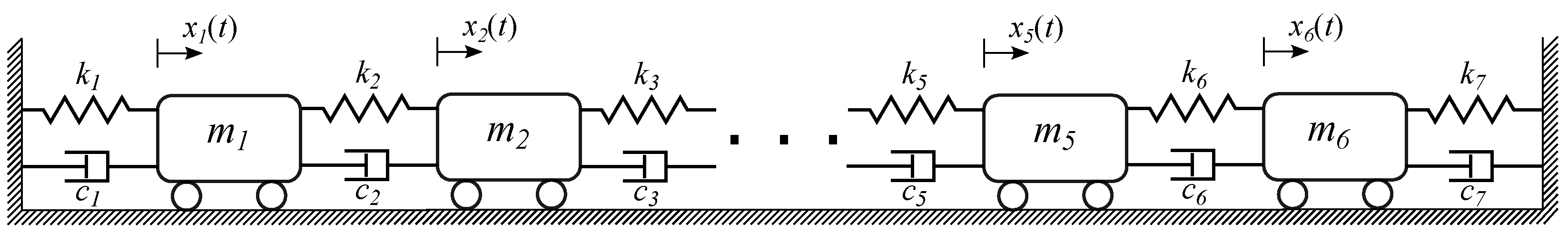
4.1. Damage Detection on a Spring-Mass-Damper System
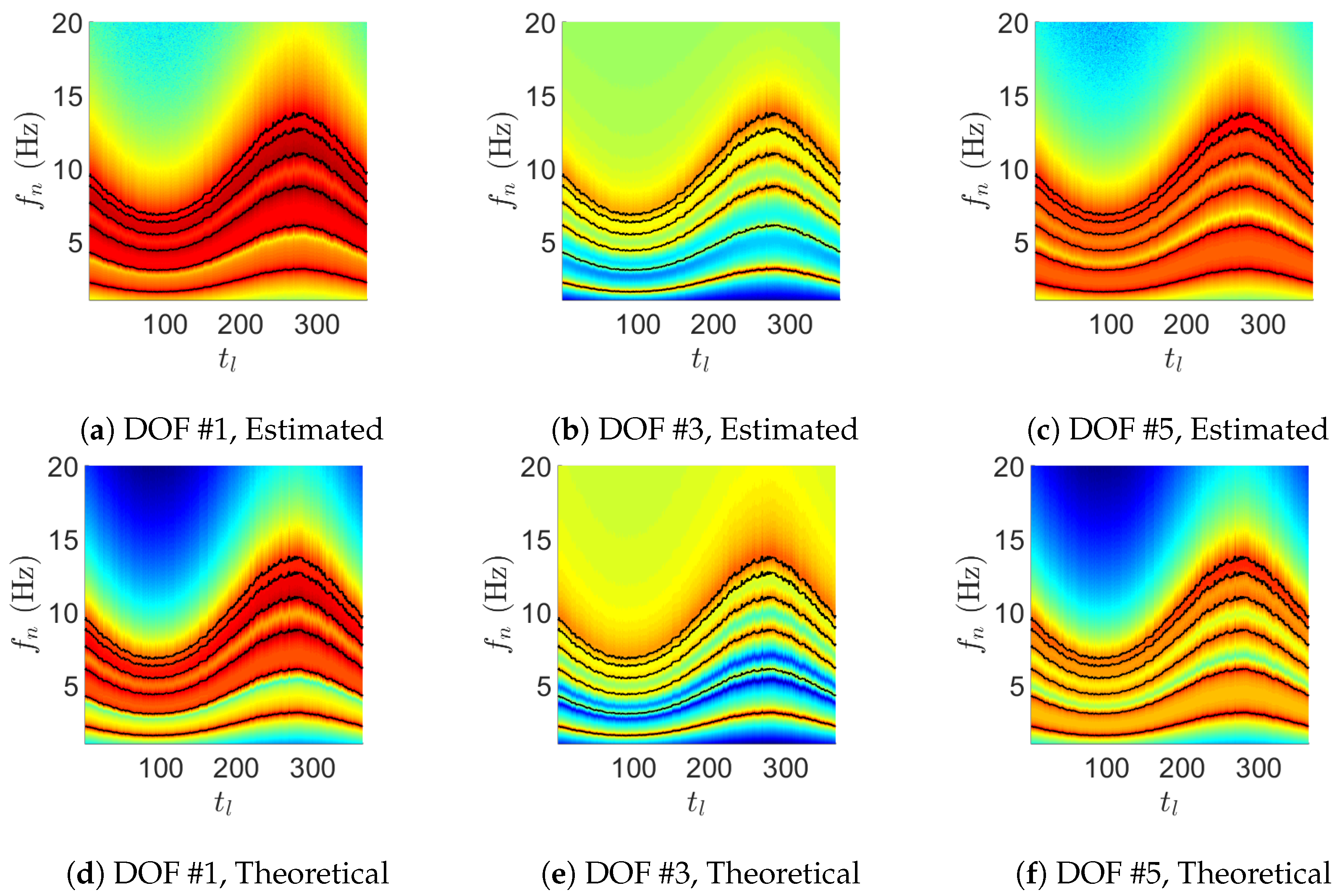
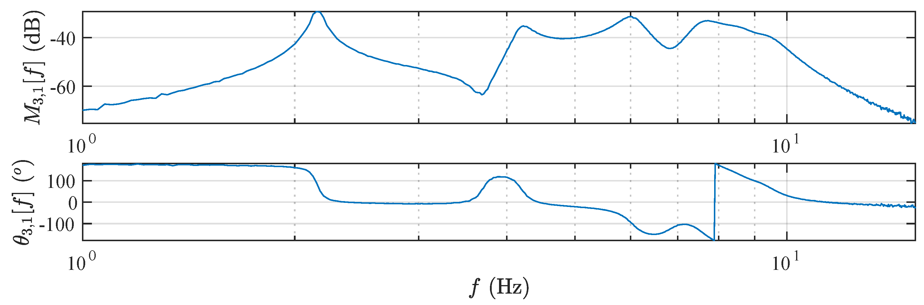
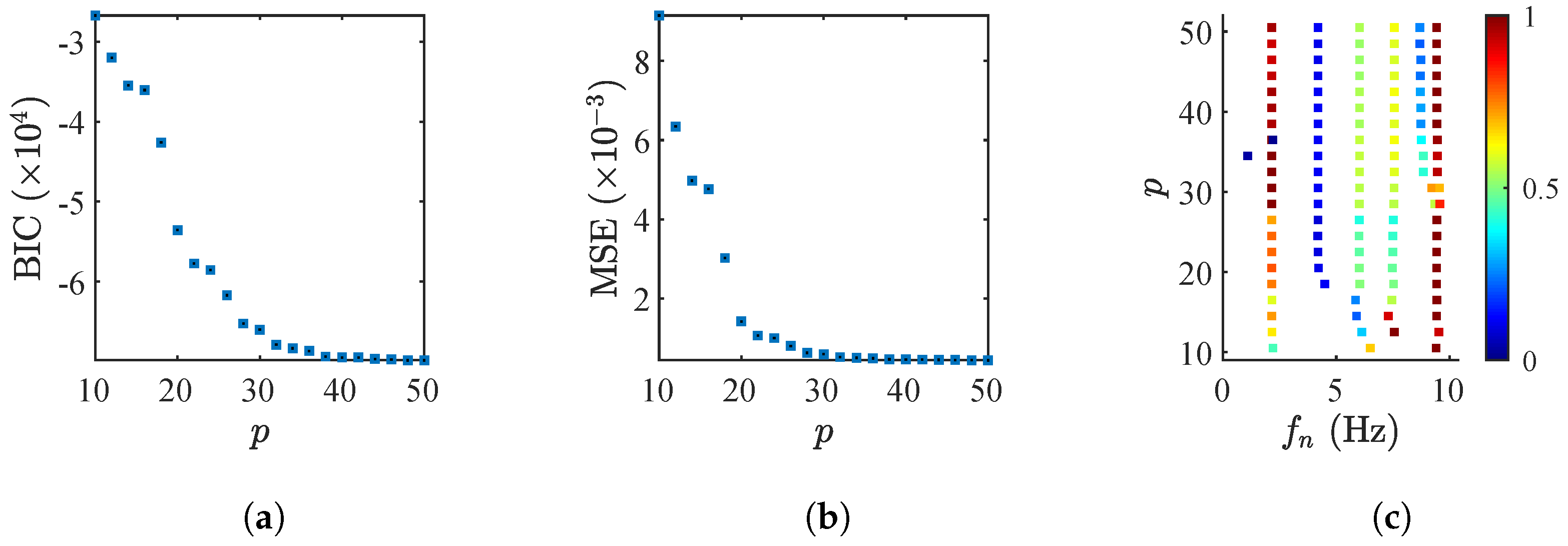
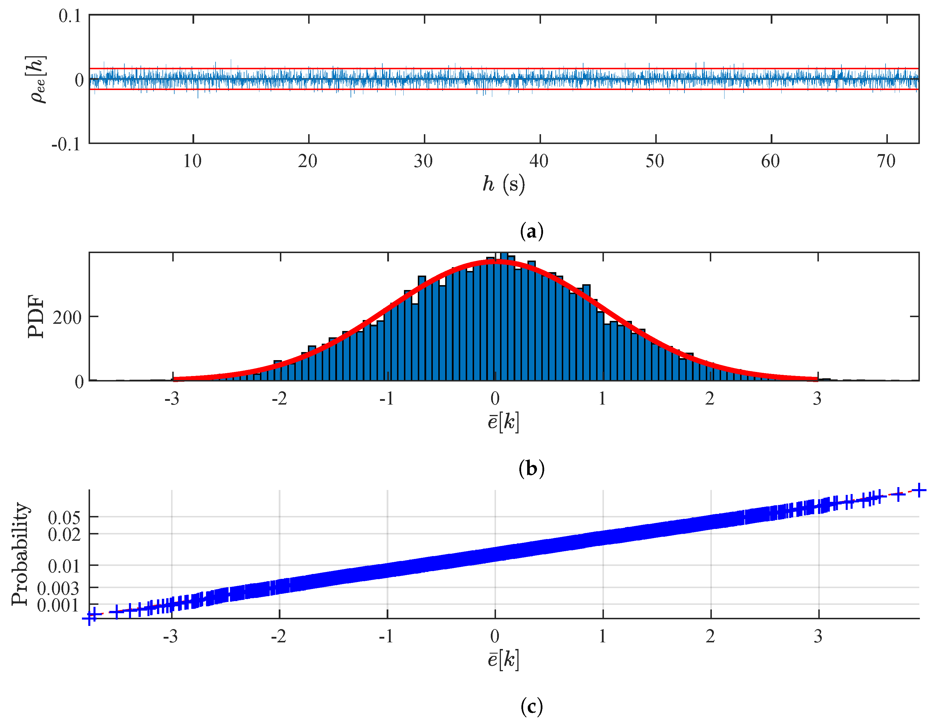
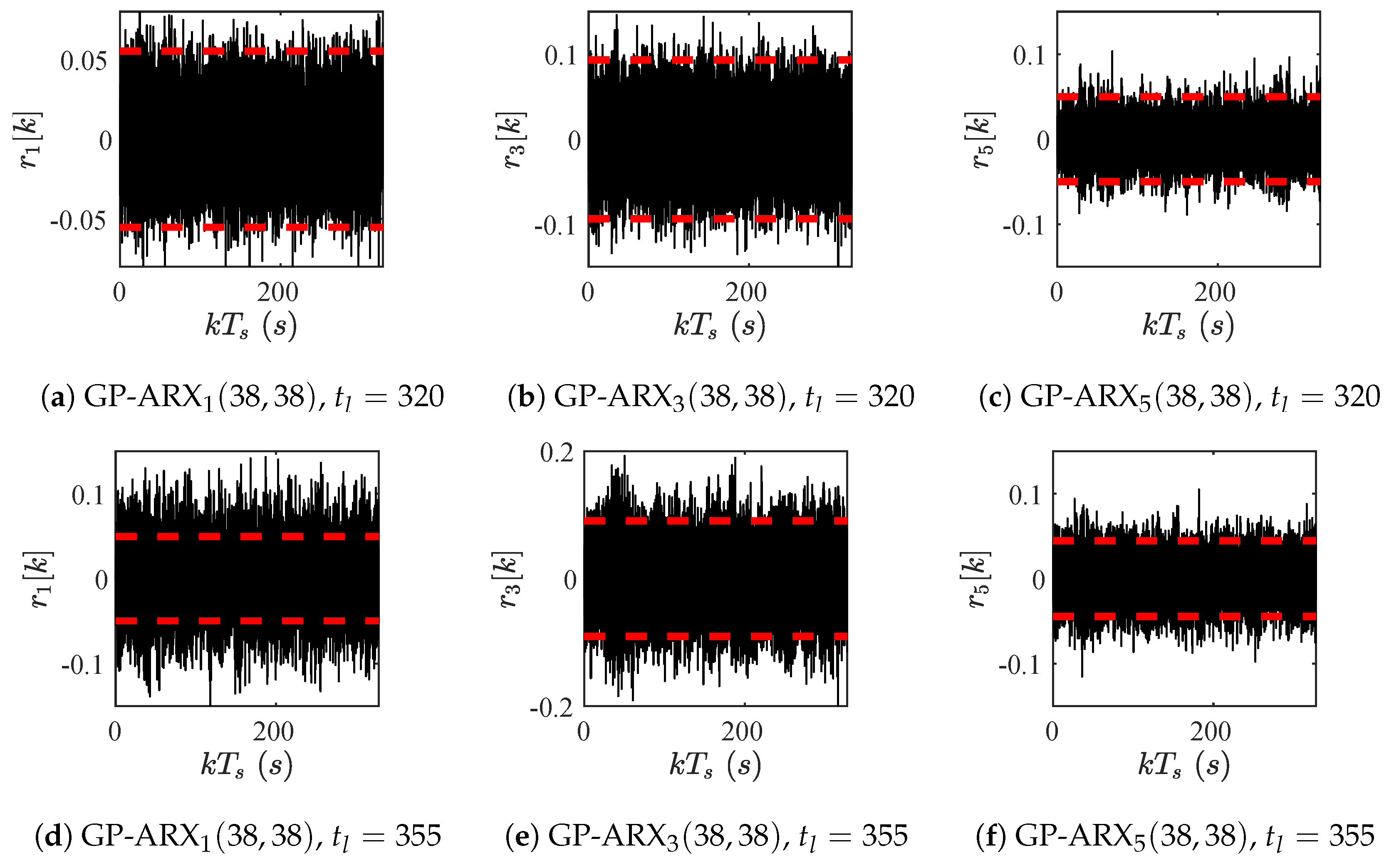
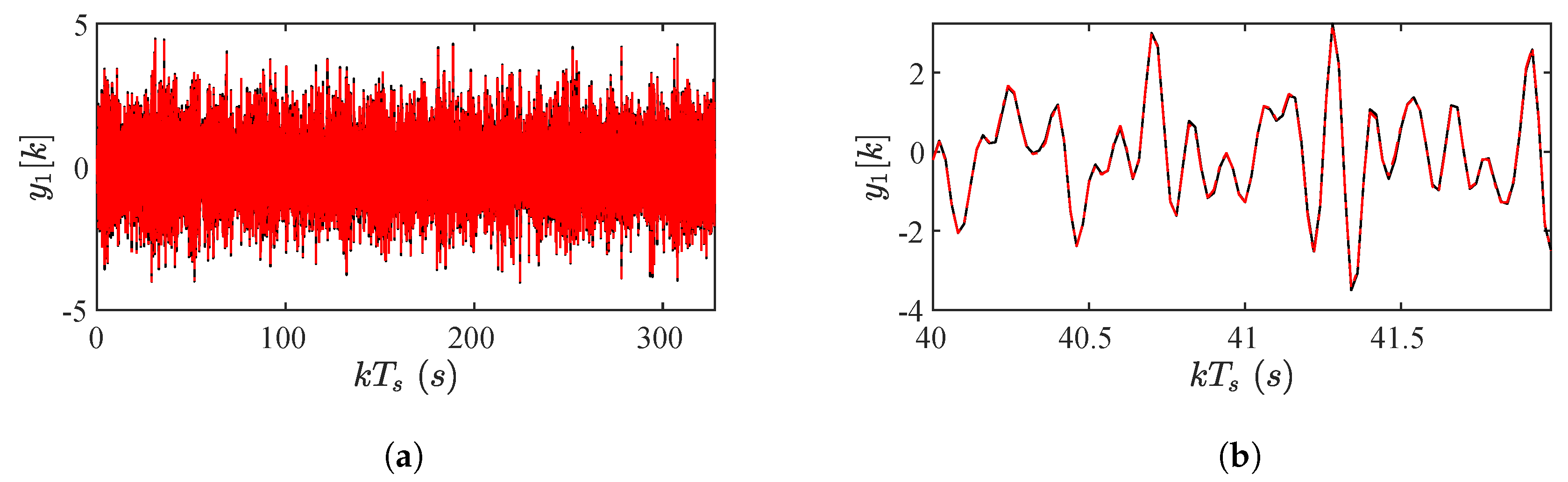
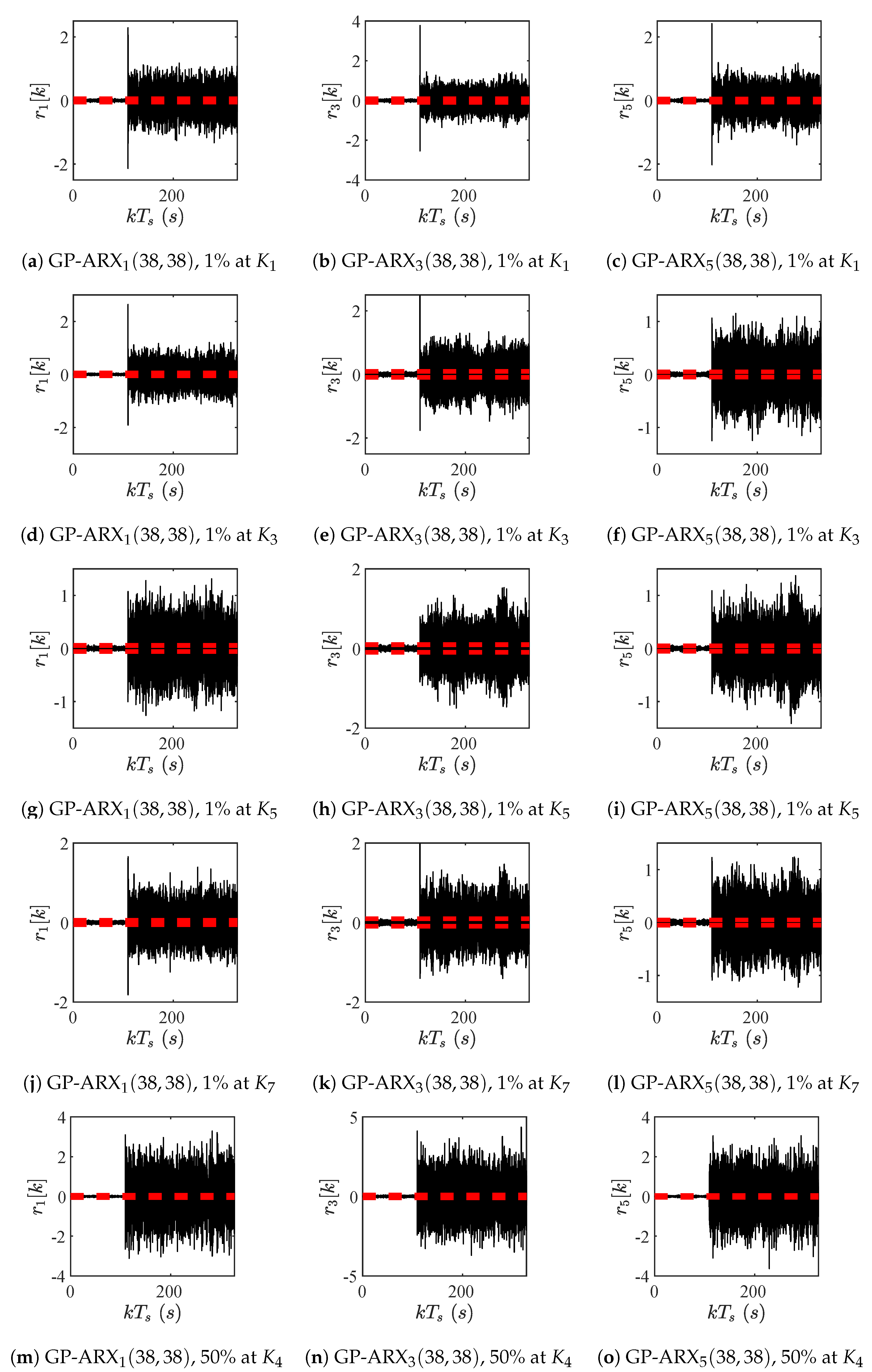
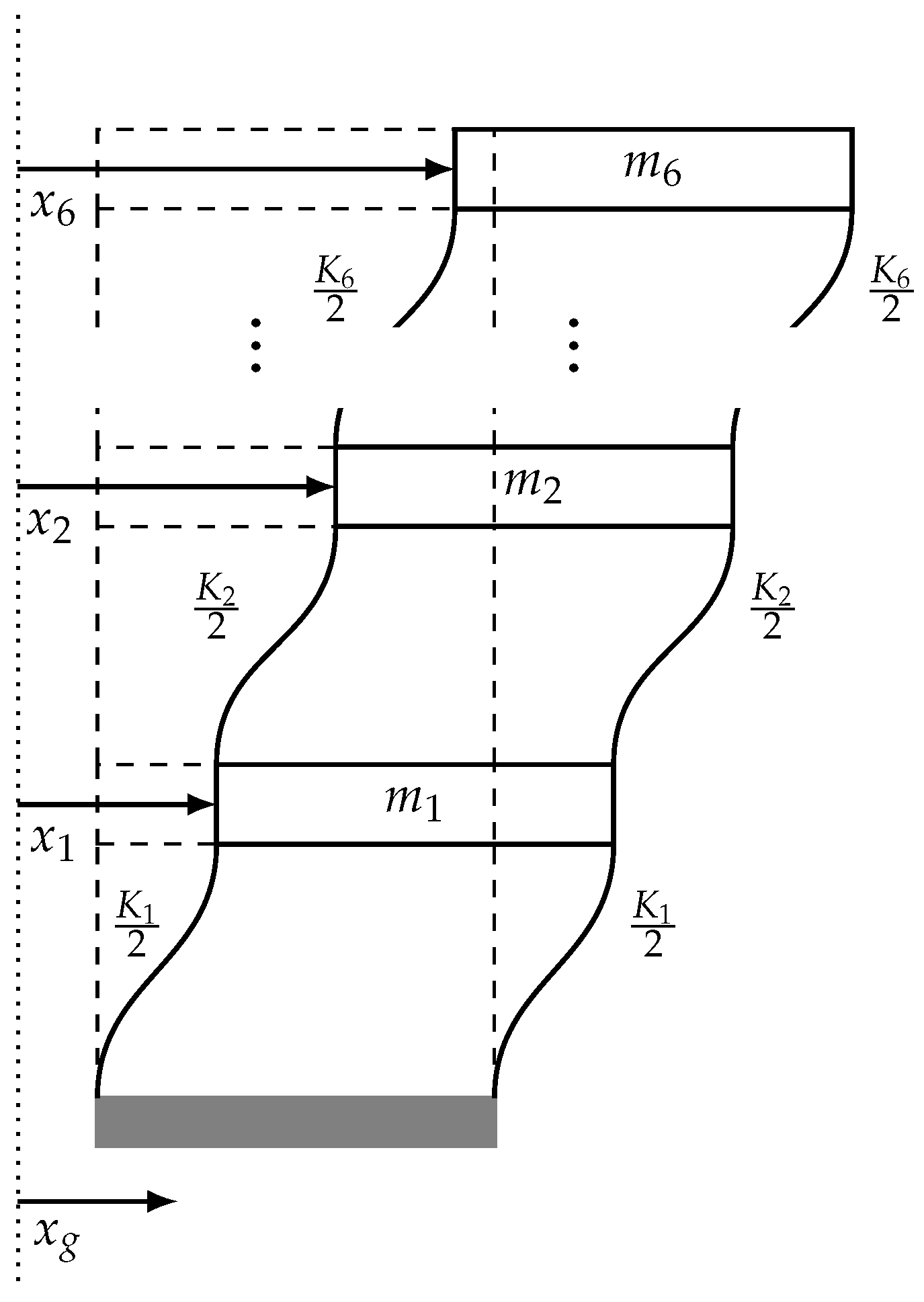
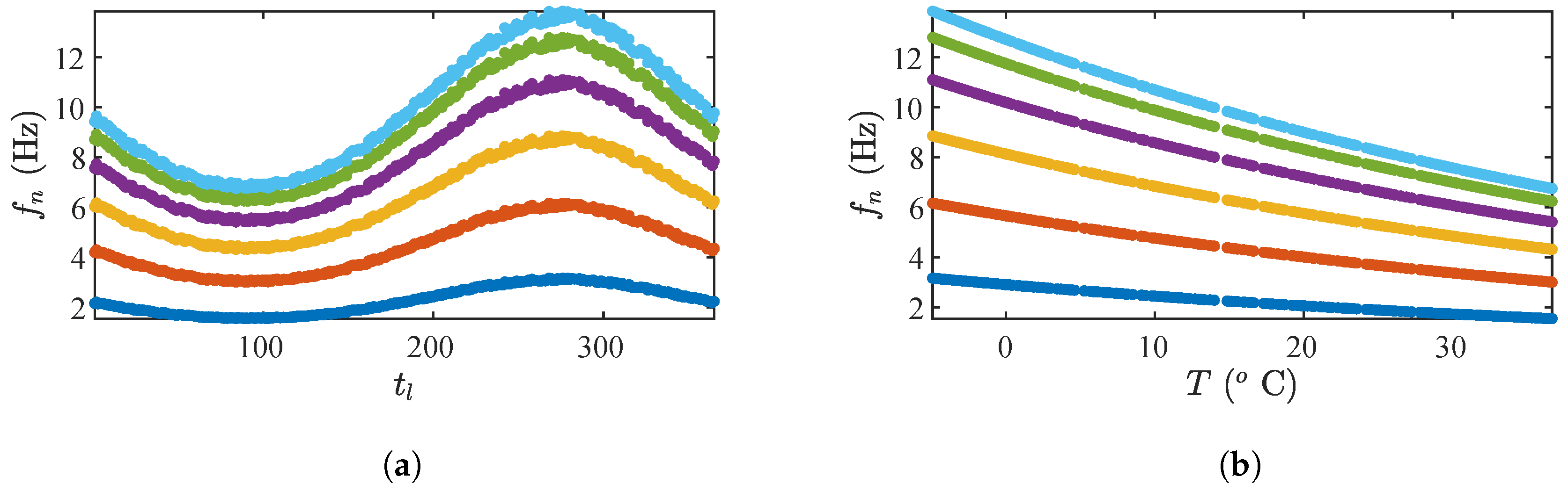
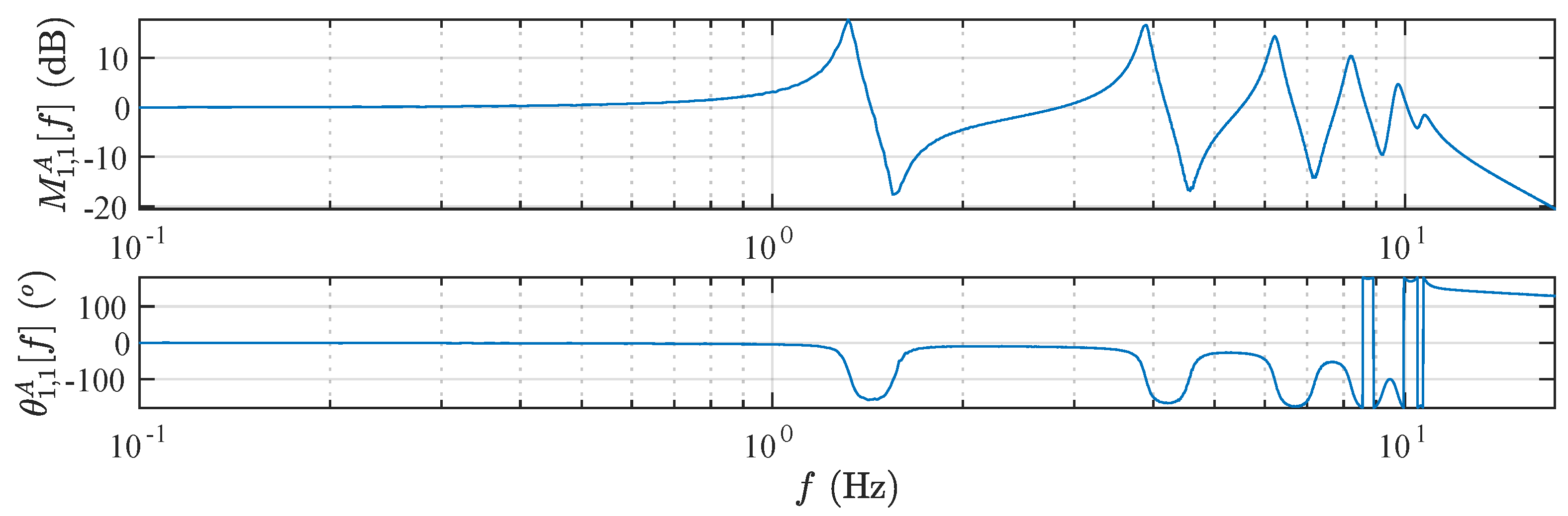
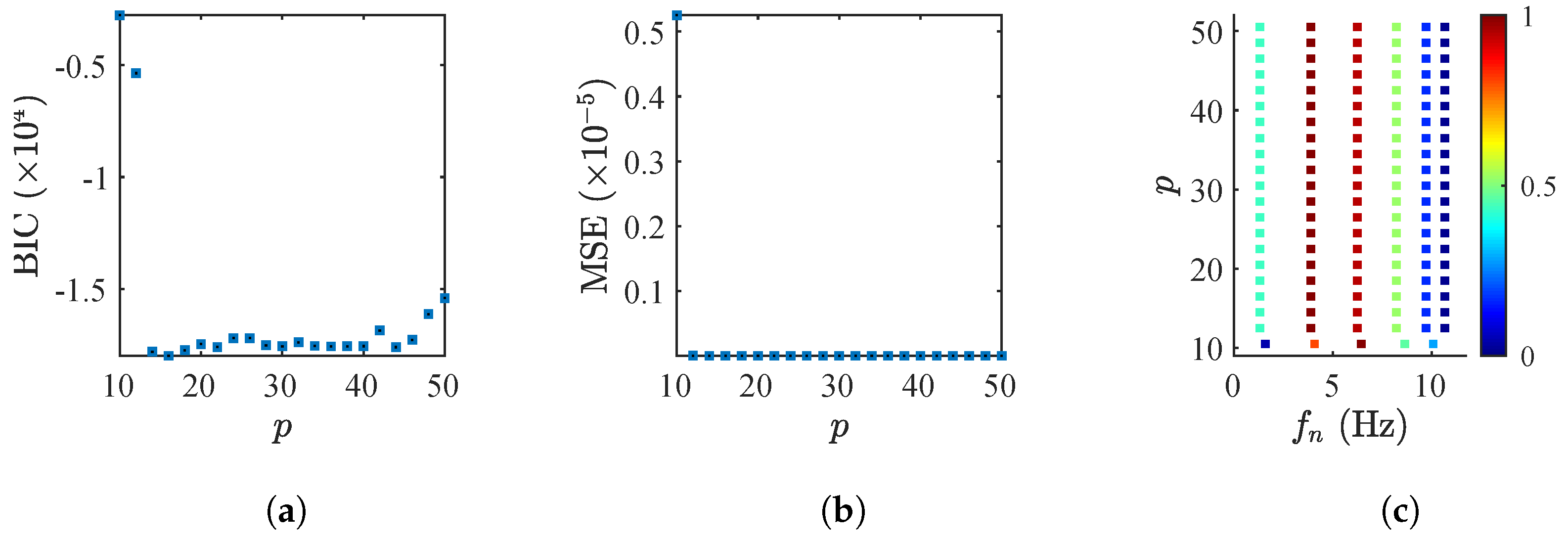
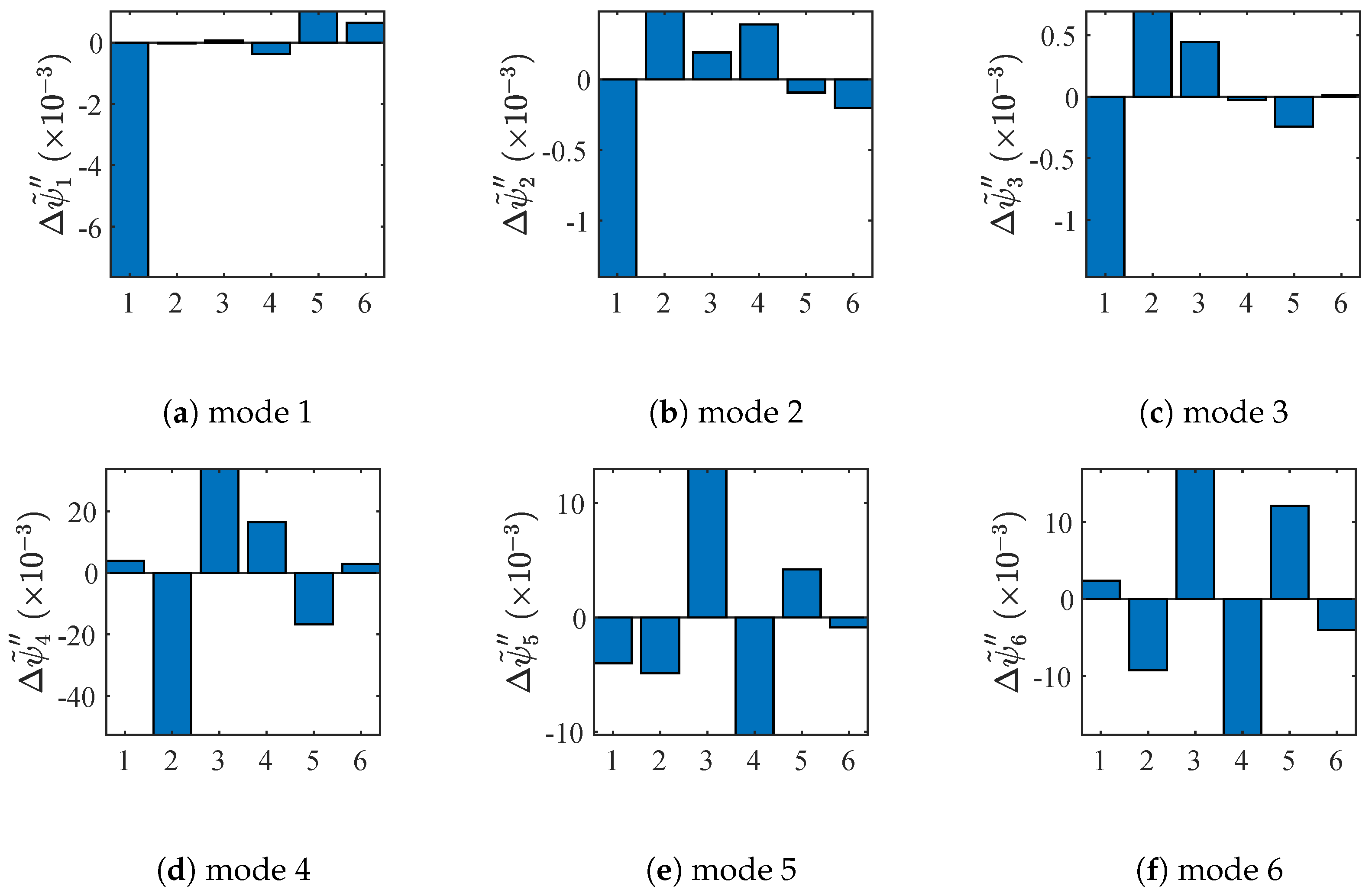
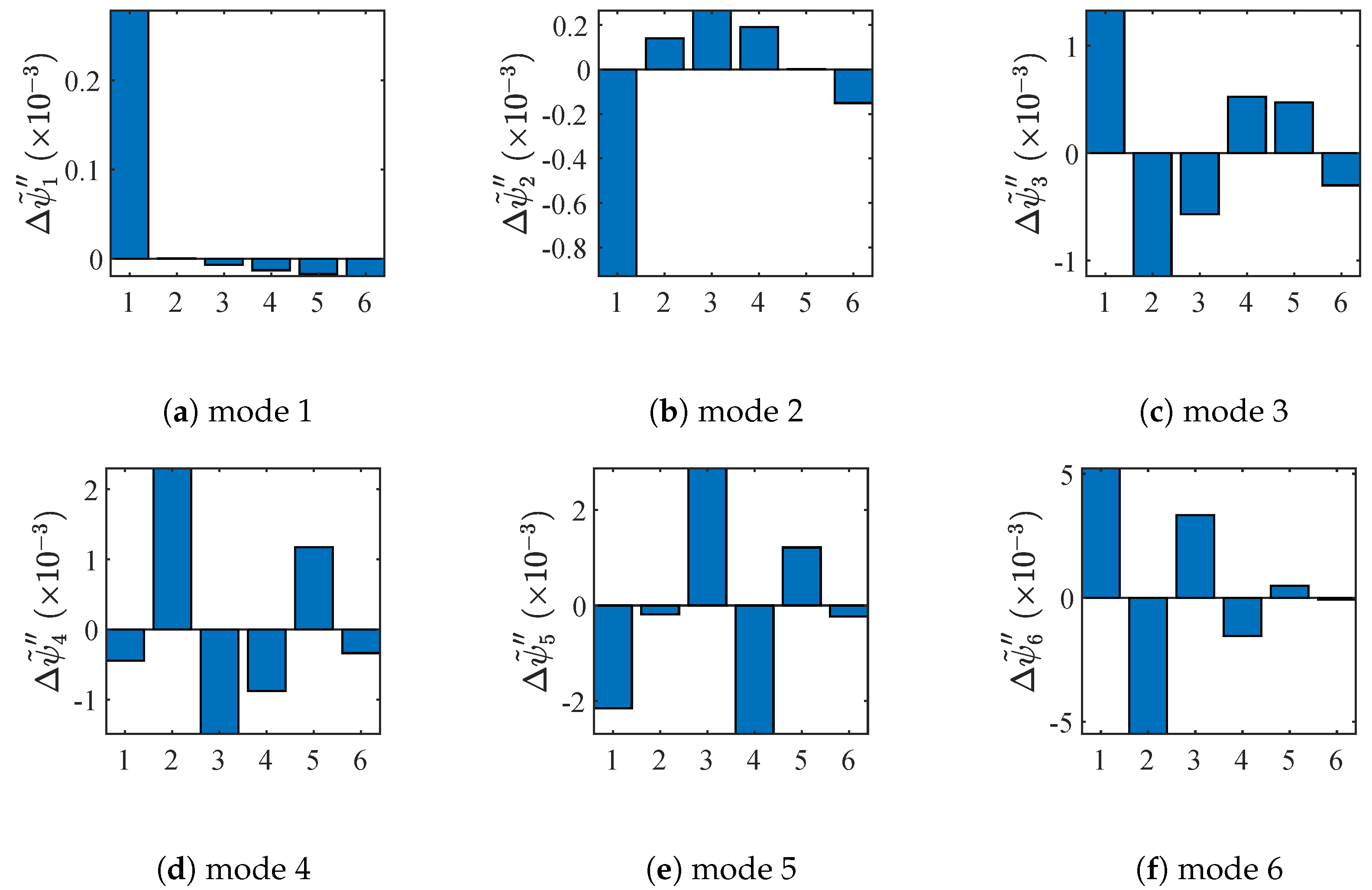
4.2. Damage Detection and Localization on a Shear Frame
5. Conclusions
Author Contributions
Funding
Conflicts of Interest
References
- Ding, S. Model-Based Fault Diagnosis Techniques: Design Schemes, Algorithms and Tools; Springer: London, UK, 2013. [Google Scholar]
- Gertler, J. Fault Detection and Diagnosis in Engineering Systems; Marcel–Dekker, Inc.: New York, NY, USA, 1998. [Google Scholar]
- Natke, H.; Cempel, C. Model—Based Fault Diagnosis of Mechanical Systems: Fundamentals, Detection, Localization, Assessment; Springer: Berlin, Germany, 1997. [Google Scholar]
- Chen, J.; Patton, R. Robust Model—Based Fault Diagnosis of Dynamic Systems; Kluwer Academic Publishers: Norwell, MA, USA, 1999. [Google Scholar]
- Kullaa, J. Development of virtual sensors to increase the sensitivity to damage. Procedia Eng. 2017, 199, 1937–1942. [Google Scholar] [CrossRef]
- Maes, K.; Lombaert, G. Fatigue monitoring of railway bridges by means of virtual sensing. In Proceedings of the Belgian and Dutch National Groups of IABSE—Young Engineers Colloquium, TU/e, Eindhoven, The Netherlands, 15–16 March 2019. [Google Scholar]
- Tatsis, K.; Dertimanis, V.; Abdallah, I.; Chatzi, E. A substructure approach for fatigue assessment on wind turbine support structures using output-only measurements. Procedia Eng. 2017, 199, 1044–1049. [Google Scholar] [CrossRef]
- Tatsis, K.; Dertimanis, V.; Chatzi, E. Response Prediction of Systems Experiencing Operational and Environmental Variability. In Computing in Civil Engineering 2019; Chapter Computing in Civil Engineering 2019: Smart Cities, Sustainability, and Resilience; ASCE: Reston, VA, USA, 2019; pp. 468–474. [Google Scholar] [CrossRef]
- Vettori, S.; Di Lorenzo, E.; Cumbo, R.; Musella, U.; Tamarozzi, T.; Peeters, B.; Chatzi, E. Kalman-based Virtual Sensing for Improvement of Service Responses Replication in Environmental Tests #8071. In Proceedings of the IMAC XXXVIII Conference, Orlando, FL, USA, 28–31 January 2019. [Google Scholar]
- Lourens, E.; Papadimitriou, C.; Gillijns, S.; Reynders, E.; Roeck, G.D.; Lombaert, G. Joint input-response estimation for structural systems based on reduced-order models and vibration data from a limited number of sensors. Mech. Syst. Signal Process. 2012, 29, 310–327. [Google Scholar] [CrossRef]
- Sedehi, O.; Papadimitriou, C.; Teymouri, D.; Katafygiotis, L.S. Sequential Bayesian estimation of state and input in dynamical systems using output-only measurements. Mech. Syst. Signal Proces. 2019, 131, 659–688. [Google Scholar] [CrossRef]
- Ou, Y.; Chatzi, E.N.; Dertimanis, V.K.; Spiridonakos, M.D. Vibration-based experimental damage detection of a small-scale wind turbine blade. Struct. Health Monit. 2017, 16, 79–96. [Google Scholar] [CrossRef]
- Xiang, J.; Lei, Y.; Wang, Y.; He, Y.; Zheng, C.; Gao, H. Structural Dynamical Monitoring and Fault Diagnosis. Shock Vib. 2015, 2015, 193831. [Google Scholar] [CrossRef]
- Wu, J.; Rudnick, E.M. Bridge fault diagnosis using stuck-at fault simulation. IEEE Trans. Comput. Aided Des. Integr. Circuits Syst. 2000, 19, 489–495. [Google Scholar] [CrossRef]
- Xiang, T.; Huang, K.; Zhang, H.; Zhang, Y.; Zhang, Y.; Zhou, Y. Detection of Moving Load on Pavement Using Piezoelectric Sensors. Sensors 2020, 20, 2366. [Google Scholar] [CrossRef]
- Alblawi, A. Fault diagnosis of an industrial gas turbine based on the thermodynamic model coupled with a multi feedforward artificial neural networks. Energy Rep. 2020, 6, 1083–1096. [Google Scholar] [CrossRef]
- Kazemi, H.; Yazdizadeh, A. Fault detection and isolation of gas turbine engine using inversion-based and optimal state observers. Eur. J. Control 2020. [Google Scholar] [CrossRef]
- Abdallah, I.; Dertimanis, V.; Mylonas, H.; Tatsis, K.; Chatzi, E.; Dervilis, N.; Worden, K.; Maguire, E. Fault Diagnosis of wind turbine structures using decision tree learning algorithms with big data. In Proceedings of the European Safety and Reliability Conference, ESREL 2018, Trondheim, Norway, 17–21 June 2018. [Google Scholar]
- Sanchez, H.; Escobet, T.; Puig, V.; Odgaard, P. Fault diagnosis of an advanced wind turbine benchmark using interval-based ARRs and observers. IEEE Trans. Ind. Electr. 2015, 62, 3783–3793. [Google Scholar] [CrossRef]
- Badihi, H.; Zhang, Y.; Hong, H. Wind Turbine Fault Diagnosis and Fault-Tolerant Torque Load Control Against Actuator Faults. IEEE Trans. Control Syst. Technol. 2015, 23, 1351–1372. [Google Scholar] [CrossRef]
- Cross, E.J.; Worden, K.; Farrar, C.R. Structural Health Monitoring for Civil Infrastructure. In Health Assessment of Engineered Structures: Bridges, Buildings and Other Infrastructures; Haldar, A., Ed.; World Scientific: Singapore, 2013; Chapter 1. [Google Scholar]
- Tcherniak, D.; Mølgaard, L.L. Vibration-based SHM System: Application to Wind Turbine Blades. J. Phys. Conf. Ser. 2015, 628, 012072. [Google Scholar] [CrossRef]
- Ou, Y.; Grauvogl, B.; Spiridonakos, M.; Dertimanis, V.; Chatzi, E.; Vidal, J. Vibration-based Damage Detection on a Blade of a Small Scale Wind Turbine. Proc. IWSHM 2015. [Google Scholar] [CrossRef]
- Dutta, A.; McKay, M.E.; Kopsaftopoulos, F.; Gandhi, F. Fault Detection and Identification for Multirotor Aircraft by Data-Driven Statistical Learning Methods. In Proceedings of the AIAA Propulsion and Energy 2019 Forum, Indianapolis, IN, USA, 19–22 August 2019. [Google Scholar] [CrossRef]
- Marzat, J.; Piet-Lahanier, H.; Damongeot, F.; Walter, E. Model-based fault diagnosis for aerospace systems: A survey. Proc. Inst. Mech. Eng. Part G J. Aerosp. Eng. 2012, 226, 1329–1360. [Google Scholar] [CrossRef]
- Giurgiutiu, V.; Zagrai, A.N. Electro-mechanical impedance method for crack detection in metallic plates. In Advanced Nondestructive Evaluation for Structural and Biological Health Monitoring; Kundu, T., Ed.; International Society for Optics and Photonics, SPIE: Washington, DC, USA, 2001; Volume 4335, pp. 131–142. [Google Scholar]
- Tashakori, S.; Baghalian, A.; Cuervo, J.; Senyurek, V.Y.; Tansel, I.N.; Uragun, B. Inspection of the machined features created at the embedded sensor aluminum plates. In Proceedings of the 2017 8th International Conference on Recent Advances in Space Technologies (RAST), Istanbul, Turkey, 19–22 June 2017; pp. 517–522. [Google Scholar]
- Xu, B.; Giurgiutiu, V. A Low-Cost and Field Portable Electromechanical (E/M) Impedance Analyzer for Active Structural Health Monitoring. In Proceedings of the 5th International Workshop on Structural Health Monitoring, Stanford University, Stanford, CA, USA, 15–17 September 2005. [Google Scholar]
- Sohn, H. Effects of environmental and operational variability on structural health monitoring. Philos. Trans. Ser. A Math. Phys. Eng. Sci. 2007, 365, 539–560. [Google Scholar] [CrossRef] [PubMed]
- Kullaa, J. Distinguishing between sensor fault, structural damage, and environmental or operational effects in structural health monitoring. Mech. Syst. Signal Proces. 2011, 25, 2976–2989. [Google Scholar] [CrossRef]
- Cross, E.; Koo, K.; Brownjohn, J.; Worden, K. Long-term monitoring and data analysis of the Tamar Bridge. Mech. Syst. Signal Proces. 2013, 35, 16–34. [Google Scholar] [CrossRef]
- Cornwell, P.; Farrar, C.; Doebling, S.; Sohn, H. Environmental variability of modal properties. Exp. Tech. 1999, 23, 45–48. [Google Scholar] [CrossRef]
- Liu, C.; De Wolf, J. Effect of temperature on modal variability of a curved concrete bridge under ambient loads. J. Struct. Eng. 2007, 133, 1742–1751. [Google Scholar] [CrossRef]
- Rohrmann, R.; Baessler, M.; Said, S.; Schmid, W.; Ruecker, W. Structural causes of temperature affected modal data of civil structures obtained by long time monitoring. In Proceedings of the IMAC XVIII—18th International Modal Analysis Conference, San Antonio, TX, USA, 7–10 February 2000. [Google Scholar]
- Bernal, D. Analytical techniques for damage detection and localization for assessing and monitoring civil infrastructures. In Sensor Technologies for Civil Infrastructures; Wang, M., Lynch, J., Sohn, H., Eds.; Woodhead Publishing: Cambridge, UK, 2014; Chapter 3; Volume 2, pp. 67–92. [Google Scholar]
- Figueiredo, E.; Park, G.; Farrar, C.; Worden, K.; Figueiras, J. Machine learning algorithms for damage detection under operational and environmental variability. Struct. Health Monit. 2011, 10, 559–572. [Google Scholar] [CrossRef]
- Harmanci, Y.; Spiridonakos, M.; Chatzi, E.; Kübler, W. An Autonomous Strain-Based Structural Monitoring Framework for Life-Cycle Analysis of a Novel Structure. Front. Built Environ. 2016, 2, 13. [Google Scholar] [CrossRef]
- Sohn, H.; Worden, K.; Farrar, C. Novelty detection under changing environmental conditions. In Proceedings of the SPIE4330: 8th Annual International Symposium on Smart Structures and Materials, Newport Beach, CA, USA, 4–8 March 2001; pp. 108–118. [Google Scholar]
- Dervilis, N.; Choi, M.; Taylor, S.; Barthorpe, R.; Park, G.; Farrar, C.; Worden, K. On damage diagnosis for a wind turbine blade using pattern recognition. J. Sound Vib. 2014, 333, 1833–1850. [Google Scholar] [CrossRef]
- Lämsä, V.; Kullaa, J. Nonlinear Factor Analysis in Structural Health Monitoring to Remove Environmental Effects. In Proceedings of the 6th International Workshop on Structural Health Monitoring, Stanford University, Stanford, CA, USA, 11–13 September 2007. [Google Scholar]
- Kullaa, J. Elimination of environmental influences from damage-sensitive features in a structural health monitoring system. In Proceedings of the First European Workshop on Structural Health Monitoring, Paris, France, 10–12 July 2002; pp. 742–749. [Google Scholar]
- Manson, G. Identifying damage sensitive, environment insensitive features for damage detection. In Proceedings of the 3rd International Conference on Identification in Engineering Systems, Swansea, UK, 15–17 April 2002; pp. 187–197. [Google Scholar]
- Reynders, E.; Wursten, G.; De Roeck, G. Output-only structural health monitoring in changing environmental conditions by means of nonlinear system identification. Struct. Health Monit. 2013. [Google Scholar] [CrossRef]
- De Boe, P.; Golinval, J. Principal component analysis of a piezosensor array for damage localization. Struct. Health Monit. 2003, 2, 137–144. [Google Scholar] [CrossRef]
- García, D.; Trendafilova, I. A multivariate data analysis approach towards vibration analysis and vibration-based damage assessment: Application for delamination detection in a composite beam. J. Sound Vib. 2014, 333, 7036–7050. [Google Scholar] [CrossRef]
- Shokrani, Y.; Dertimanis, V.K.; Chatzi, E.N.; Savoia, N.M. On the use of mode shape curvatures for damage localization under varying environmental conditions. Struct. Control Health Monit. 2018, 25, e2132. [Google Scholar] [CrossRef]
- Ou, Y.W.; Dertimanis, V.K.; Chatzi, E.N. Operational Damage Localization of Wind Turbine Blades. In Experimental Vibration Analysis for Civil Structures; Conte, J.P., Astroza, R., Benzoni, G., Feltrin, G., Loh, K.J., Moaveni, B., Eds.; Springer International Publishing: Cham, Switzerland, 2018; pp. 261–272. [Google Scholar]
- Dervilis, N.; Worden, K.; Cross, E. On robust regression analysis as a means of exploring environmental and operational conditions for SHM data. J. Sound Vib. 2015, 347, 279–296. [Google Scholar] [CrossRef]
- Dervilis, N.; Zhang, T.; Bull, L.; Cross, E.; Rogers, T.; Fuentes, R.; Dertimanis, V.; Abdallah, I.; Chatzi, E.; Worden, K. A nonlinear robust outlier detection approach for SHM. In Proceedings of the IOMAC 2019, Copenhagen, Denmark, 13–15 May 2019. [Google Scholar]
- Toth, R. Modeling and Identification of Linear Parameter-Varying Systems; Lecture Notes in Control and Information Sciences; Springer: Berlin/Heidelberg, Germany, 2010. [Google Scholar] [CrossRef]
- Avendaño-Valencia, L.D.; Chatzi, E.N.; Koo, K.Y.; Brownjohn, J.M. Gaussian Process Time-Series Models for Structures under Operational Variability. Front. Built Environ. 2017, 3, 69. [Google Scholar] [CrossRef]
- Kopsaftopoulos, F.; Nardari, R.; Li, Y.H.; Chang, F.K. A stochastic global identification framework for aerospace structures operating under varying flight states. Mech. Syst. Signal Proces. 2018, 98, 425–447. [Google Scholar] [CrossRef]
- Sakellariou, J.; Fassois, S. Functionally Pooled models for the global identification of stochastic systems under different pseudo-static operating conditions. Mech. Syst. Signal Proces. 2016, 72–73, 785–807. [Google Scholar] [CrossRef]
- Spiridonakos, M.D.; Chatzi, E.N.; Sudret, B. Polynomial Chaos Expansion Models for the Monitoring of Structures under Operational Variability. ASCE-ASME J. Risk Uncertain. Eng. Syst. Part A Civ. Eng. 2016, 2, B4016003. [Google Scholar] [CrossRef]
- Spiridonakos, M.D.; Chatzi, E.N. Stochastic Structural Identification from Vibrational and Environmental Data. In Encyclopedia of Earthquake Engineering; Beer, M., Kougioumtzoglou, I.A., Patelli, E., Au, I.S.K., Eds.; Springer: Berlin/Heidelberg, Germany, 2014. [Google Scholar] [CrossRef]
- Avendaño-Valencia, L.D.; Fassois, S.D. Natural vibration response based damage detection for an operating wind turbine via Random Coefficient Linear Parameter Varying AR modelling. J. Phys. Conf. Ser. 2015, 628, 012073. [Google Scholar] [CrossRef]
- Bogoevska, S.; Spiridonakos, M.; Chatzi, E.; Dumova-Jovanoska, E.; Höffer, R. A Data-Driven Diagnostic Framework for Wind Turbine Structures: A Holistic Approach. Sensors 2017, 17, 720. [Google Scholar] [CrossRef]
- Avendaño-Valencia, L.D.; Fassois, S.D. Gaussian Mixture Random Coefficient model based framework for SHM in structures with time–dependent dynamics under uncertainty. Mech. Syst. Signal Proces. 2017, 97, 59–83. [Google Scholar] [CrossRef]
- Avendaño-Valencia, L.D.; Fassois, S.D. Damage/fault diagnosis in an operating wind turbine under uncertainty via a vibration response Gaussian mixture random coefficient model based framework. Mech. Syst. Signal Proces. 2017, 91, 326–353. [Google Scholar] [CrossRef]
- Avendaño-Valencia, L.D.; Chatzi, E.N. Sensitivity driven robust vibration-based damage diagnosis under uncertainty through hierarchical Bayes time-series representations. Procedia Eng. 2017, 199, 1852–1857. [Google Scholar] [CrossRef]
- Demetriou, M.A. Using unknown input observers for robust adaptive fault detection in vector second-order systems. Mech. Syst. Signal Proces. 2005, 19, 291–309. [Google Scholar] [CrossRef]
- Basseville, M. Information criteria for residual generation and fault detection and isolation. Automatica 1997, 33, 783–803. [Google Scholar] [CrossRef]
- Isermann, R. Fault-Diagnosis Systems: An Introduction from Fault Detection to Fault Tolerance; Springer: Berlin, Germany, 2006. [Google Scholar]
- Simani, S.; Fantuzzi, C.; Patton, R. Model–Based Fault Diagnosis in Dynamic Systems Using Identification Techniques; Springer: London, UK, 2003. [Google Scholar]
- Dertimanis, V.; Giagopoulos, D.; Chatzi, E. Finite Element Metamodelling of Uncertain Structures. In Proceedings of the ECCOMAS 2016, Crete, Greece, 5–10 June 2016; pp. 6316–6327. [Google Scholar]
- Spiridonakos, M.; Dertimanis, V.; Chatzi, E. Estimation of Data-Driven Polynomial Chaos using Hybrid Evolution Strategies. In Proceedings of the Fourth International Conference on Soft Computing Technology in Civil, Structural and Environmental Engineering; Tsompanakis, Y., Kruis, J., Topping, B., Eds.; Civil-Comp Press: Stirlingshire, UK, 2015; p. 24. [Google Scholar] [CrossRef]
- Dertimanis, V.; Spiridonakos, M.; Chatzi, E. Data-driven uncertainty quantification of structural systems via B-spline expansion. Comput. Struct. 2018, 207, 245–257. [Google Scholar] [CrossRef]
- Box, G.; Jenkins, G.; Reinsel, G. Time Series Analysis, Forecasting and Control, 4th ed.; John Wiley & Sons Ltd.: Chichester, UK, 2013. [Google Scholar]
- Dertimanis, V.K.; Koulocheris, D.V. VAR Based State–space Structures: Realization, Statistics and Spectral Analysis. In Lecture Notes in Electrical Engineering; Cetto, J.A., Filipe, J., Ferrier, J.L., Eds.; Springer: Berlin/Heidelberg, Germany, 2011; Volume 85, pp. 301–315. [Google Scholar]
- Dertimanis, V.K. On the use of dispersion analysis for model assessment in structural identification. J. Vib. Control 2013, 19, 2270–2284. [Google Scholar] [CrossRef]
- Dertimanis, V.K.; Chatzi, E. Dispersion-corrected stabilization diagrams for model order assessment in structural identification. In Proceedings of the 7th European Workshop on Structural Health Monitoring, EWSHM 2014, Nantes, France, 8–11 July 2014; pp. 2159–2166. [Google Scholar]
- Dertimanis, V.K.; Spiridonakos, M.D.; Chatzi, E.N. Dispersion–Corrected, Operationally Normalized Stabilization Diagrams for Robust Structural Identification. In Model Validation and Uncertainty Quantification; Atamturktur, H.S., Moaveni, B., Papadimitriou, C., Schoenherr, T., Eds.; Springer International Publishing: Cham, Switzerland, 2015; Volume 3, pp. 75–83. [Google Scholar] [CrossRef]
- Pandey, A.; Biswas, M.; Samman, M. Damage detection from changes in curvature mode shapes. J. Sound Vib. 1991, 145, 321–332. [Google Scholar] [CrossRef]
- Avendaño-Valencia, L.D.; Chatzi, E.N. Multivariate GP-VAR models for robust structural identification under operational variability. Probabilistic Eng. Mech. 2020, 60, 103035. [Google Scholar] [CrossRef]


| ARX | ARX | ARX | |
|---|---|---|---|
| 98.91% | 98.93% | 98.91% | |
| Quantity | AR Parameters | Exogenous Parameters | Noise Variance |
|---|---|---|---|
| Basis Function Type | Discrete Fourier | Polynomial | |
| Basis Function Formula | , | , | |
| , | |||
| Kernel Type | Matérn 3/2 | ||
| Kernel Formula | |||
| Order | |||
| GP-ARX | GP-ARX | GP-ARX | |
|---|---|---|---|
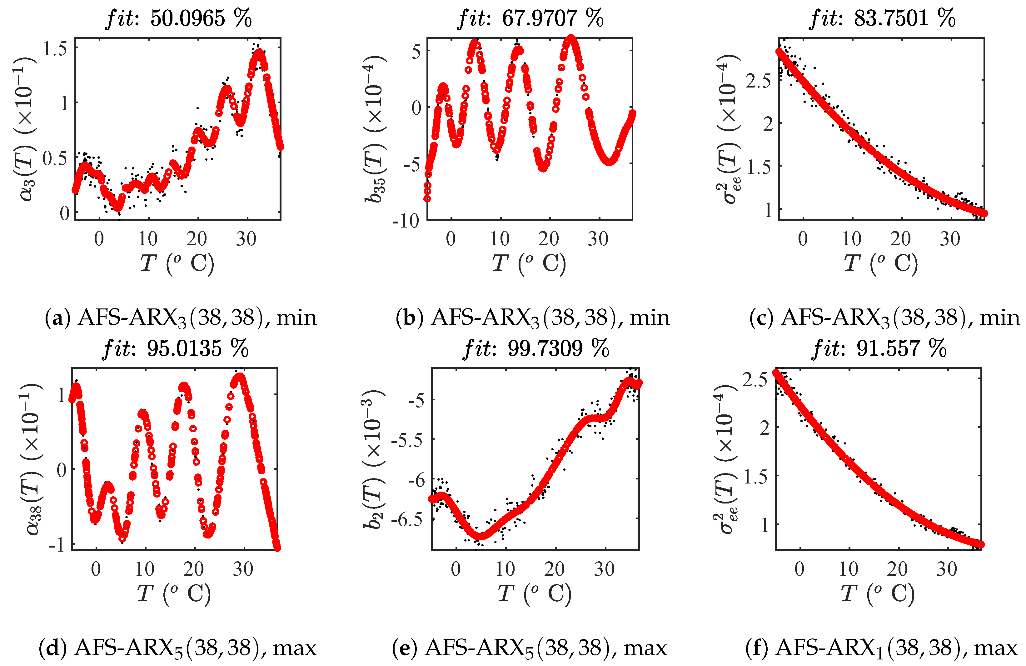
| 91.56% | 83.75% | 85.37% |
| ARX | ARX | ARX | ARX | ARX | ARX | |
|---|---|---|---|---|---|---|
| 99.97% | 99.98% | 99.99% | 99.98% | 99.98% | 98.98% | |
| Quantity | AR Parameters | Exogenous Parameters | Noise Variance |
|---|---|---|---|
| Basis function type | polynomial | discrete Fourier | |
| Basis function formula | as in Table 2 | as in Table 2 | |
| Kernel type | Matérn 3/2 | ||
| Kernel formula | as in Table 2 | ||
| Order | |||
| ARX | ARX | ARX | ARX | ARX | ARX | |
|---|---|---|---|---|---|---|
| 16.42% | 16.49% | 16.70% | 16.79% | 16.83% | 16.74% |
© 2020 by the authors. Licensee MDPI, Basel, Switzerland. This article is an open access article distributed under the terms and conditions of the Creative Commons Attribution (CC BY) license (http://creativecommons.org/licenses/by/4.0/).
Share and Cite
Tatsis, K.; Dertimanis, V.; Ou, Y.; Chatzi, E. GP-ARX-Based Structural Damage Detection and Localization under Varying Environmental Conditions. J. Sens. Actuator Netw. 2020, 9, 41. https://doi.org/10.3390/jsan9030041
Tatsis K, Dertimanis V, Ou Y, Chatzi E. GP-ARX-Based Structural Damage Detection and Localization under Varying Environmental Conditions. Journal of Sensor and Actuator Networks. 2020; 9(3):41. https://doi.org/10.3390/jsan9030041
Chicago/Turabian StyleTatsis, Konstantinos, Vasilis Dertimanis, Yaowen Ou, and Eleni Chatzi. 2020. "GP-ARX-Based Structural Damage Detection and Localization under Varying Environmental Conditions" Journal of Sensor and Actuator Networks 9, no. 3: 41. https://doi.org/10.3390/jsan9030041
APA StyleTatsis, K., Dertimanis, V., Ou, Y., & Chatzi, E. (2020). GP-ARX-Based Structural Damage Detection and Localization under Varying Environmental Conditions. Journal of Sensor and Actuator Networks, 9(3), 41. https://doi.org/10.3390/jsan9030041