Article

Monitoring System of a Heat Pump Installation for Heating a Rural House Using Low-grade Heat from a Surface Watercourse

by
Valeriy Kharchenko
1,
Arseniy Sychov
1,
Pasquale Luigi De Angelis
2 and
Ugo Fiore
2,*
1
FSBSI Federal Scientific Agroengineering Center VIM, 1st Institutsky proezd, 5, 109456 Moscow, Russia
2
Department of Management and Quantitatve Studies, Parthenope University, 80133 Naples, Italy
*
Author to whom correspondence should be addressed.
J. Sens. Actuator Netw. 2020, 9(1), 11; https://doi.org/10.3390/jsan9010011
Submission received: 20 December 2019 / Revised: 30 January 2020 / Accepted: 7 February 2020 / Published: 9 February 2020
(This article belongs to the Special Issue Advanced Instrumentation for Power Converter Applications)

Abstract

:
Increasing the efficiency of heat pump systems primarily used for heat supply to buildings is an important topic. This is especially true for systems constructed according to non-standard schemes and which use low-grade heat from various sources that are rarely considered for these purposes. Such studies require special, often expensive, data acquisition systems. In this paper, a low-cost computer-based monitoring system is presented. The monitoring system incorporates solutions which are new or seldom used. It is shown that modern semiconductor thermistors can replace commonly used platinum temperature sensors and thermocouples. A proposal for processing frequency output signals from sensors through an analog-to-digital converter and a way to reduce the number of required input channels are described. The monitoring system allows optimization of various types of heat-pump-based installations. The system has been used for quite a long time to monitor the operation of the heat pump installation using low-grade heat from a surface watercourse. With its help, the feasibility of using the previously proposed submersible floating heat exchanger is justified and the optimal scheme for its placement in the watercourse is determined.

1. Introduction

Increasing the use of renewable energy sources is of a great importance nowadays. A significant proportion of the total cost of energy resources relates to the heat supply for the residential sector. Therefore, introducing schemes using renewable energy for this purpose is a topic deserving attention.
In particular, the following directions for solving this problem can be identified:
-
the use of energy from renewable fuel resources (biogas, pellets, etc.);
-
the use of high-grade energy received from the Sun or the Earth’s interior, directly or through conversion into electrical energy;
-
the use of low-grade heat, both natural and anthropogenic waste, through conversion by means of heat pumps.
In the latter case, it is possible to combine low-grade energy and energy received from renewable sources to drive the heat pump [1]. Moreover, devices for generating electricity based on renewable sources and heat pumps consuming this energy may not be located next to each other, but, for example, be part of the same microgrid [2]. This approach has enormous potential, and it is currently far from being realized to its fullest extent. Leveraging the potential of environmental warmth for the purpose of housing heating seems attractive, and the use of heat pumps makes this task feasible.
In many countries of the world, heat pump installations (HPI) have been actively used in the field of heat supply for a long time, especially for heat supply to private houses. HPIs can have different schemes for the extraction of low-grade and distribution of high-grade heat. Various schemes for the low-grade heat extraction are developed for different heat source types and conditions. Traditional sources of low-grade heat for heat pumps are mainly ambient air, soil or groundwater.
Heat pump installations using the heat of ambient air usually do not require a low-temperature circuit with an intermediate heat carrier. Therefore, they are characterized by low cost. These pump installations are common in countries with a relatively mild climate. In countries with low temperatures in the cold season, such installations are not very effective [3].
HPIs which use the heat of the soil or groundwater are more universal. Generally, when using heat of the soil, a circuit with an intermediate heat carrier is organized to absorb heat and transfer it to the heat pump evaporator. For heat extraction, either schemes based on laying pipes over a large area at a depth of 1.5–2 m or schemes which entail drilling wells and organizing vertical or inclined probes in them are usually adopted. The use of low-grade heat from groundwater also requires drilling at least two wells [4,5]. A disadvantage of such solutions is the significant complexity and consequently the high cost of preparatory work. Nevertheless, this option for the organization of heat supply has gained sufficient diffusion in Europe, North America and other parts of the world.
It seems promising to use low-grade heat of surface water bodies and streams where they are available near the installation to be heated. HPIs, which use the heat of such sources are still rare and no universal solutions has been developed for extracting heat from environmental water [6,7,8]. One of the known schemes extracts heat via a plastic pipe bay or a frame with lengthy plastic pipes attached to it at the bottom of a pond or a watercourse. However, such a scheme was found to be far from optimal in many cases, especially when it comes to using the heat of watercourses. For such cases, a special submersible floating water-brine heat exchanger has been suggested [9], which is embedded into an intermediate heat carrier (brine) circuit (Figure 1).
Depending on local conditions, various schemes for placing this heat exchanger in the channel are possible. The basic principle is to place it across the flow in its core, in order to intensify heat transfer and thus to increase the efficiency of the whole HPI. In general, the diffusion of heat pump systems is complicated, largely because a high investment with a rather long payback period is required. Both the amount and the return time of the investment depend on the energy efficiency of HPI, and therefore the technical and economic optimization of such installations is of particular importance.
For the design of systems using the low-grade heat of surface water, more in-depth studies on heat extraction from water are needed. Near-zero Celsius temperatures are of great importance, since under such conditions there is a high probability of heat-exchange surfaces icing. If the system is improperly designed, the process of icing can have a significant negative effect on efficiency and operability. To conduct such studies and optimize technical devices, first of all, special means of monitoring of the operation of HPI are required.
Traditionally, data acquisition (DAQ) systems based on various DAQ devices are used to solve such problems [10,11,12,13,14]. The main measured parameters for working with heat pumps systems are temperature and liquid flow rate. In some cases, pressure is also measured [14,15]. Two types of temperature sensors are commonly used in such systems: platinum resistance temperature detectors (Pt100) [10,11,13,14,15] and thermocouples (K or T-type) [12,13,16,17]. Mass flow meters (Coriolis flow meter) [11,14] or volumetric flow meters (including electromagnetic and ultrasonic types) [10,12,13] are used to measure flow rate.
It is not always possible to install expensive equipment in remote locations, such as rural areas, and to use it for a long time. Faced with this, we developed a monitoring system based on inexpensive elements, the accuracy of which is, however, sufficient to identify the dependencies of interest. In this article, the lessons learned from the creation and practical use of a monitoring system of a heat pump installation for heating a rural house using low-grade heat from a surface watercourse is described.

2. Materials and Methods

2.1. A Brief Description of the Entire Heating System

The heat supply system is an experimental installation on which various technical solutions were worked out. The monitoring system is designed to analyze the operation of a heat pump heating system in various operating modes using various designs of its individual elements. In addition, when the entire heat supply system is put into trial operation, the monitoring system is used to obtain the primary information necessary to organize the management of its work in order to find optimal operating modes.
The heating system was designed and built in the Moscow region. It is intended for heating a country house. The watercourse, which is a source of low-grade heat, flows 40 m away from the heated house. A schema of the territory with a heated house located on it, a watercourse with a heat exchanger installed on it, photographed using a quadcopter, is presented in Figure 2.
To extract heat from the watercourse, a specific heat exchanger is used, whose computer-aided-design model is shown in Figure 3.

2.2. Monitoring System: Hardware, Sensors

The monitoring system is developed to study the operation modes of the rural house heating system. For a complete analysis of the operation of the HPI, it is necessary to simultaneously monitor many operating parameters. In addition, it is required to monitor in real time such resulting parameters as the heat output and coefficient of performance (COP) of the installation. These parameters cannot be measured directly, but can only be calculated on the basis of other data. In this regard, a special system is developed for monitoring the operation parameters of the heat pump installation with the possibility of obtaining the values of performance indicators and work efficiency in real time.
The monitoring system is built on the basis of an analog-to-digital converter (ADC) L-Card E-154 with eight single-phase inputs with a common ground formed by switching input lines using an electronic switch. Despite the low cost, (lower than almost all industrial analog input modules), it has sufficient 12-bit resolution (4096 quantization levels), maximum conversion frequency 120 kHz, accuracy ±0.1% in the range of ±5 V. It is a full-featured laboratory measuring device, unlike, for example, Arduino boards, which are capable of playing the role of an ADC. However, due to the non-standard nature of the task, it is accomplished according to our developed original scheme and involves a special data processing algorithm using the plugin for a personal computer written for this purpose.
In order to calculate the COP value of HPI, it is necessary to determine the generated heat flow Q H and the consumed electric power W and then find their ratio, which is the standard calculation formula for COP of heat pumps:
C O P = Q H W .
Measurement of electric power is not difficult and there are many meters of various accuracy classes for this purpose. In our case, we use an electronic meter of electric power and spent electricity Mercuriy 200.1 with a pulse output and an accuracy of ±1.5%.
The method for determining heat production depends on the heat power installation scheme, namely, on the presence or absence of intermediate heat carrier circuits. Heat pumps without such circuits are not considered for the organization of the described monitoring system. In the case of the presence of a liquid circuit for the distribution of generated heat, it is possible to determine the generation Q H with fairly high accuracy by measuring the temperature of the heat carrier at the inlet T i n and outlet T o u t of the heat pump condenser and the mass flow rate G M of the heat carrier:
Q H = G M · C h c · T i n T o u t ,
where C h c is the specific heat capacity of the high temperature heat carrier.
In the case of a water-to-air heat pump, it is not possible to directly measure the output using the available measuring instruments, but it is possible to calculate it based on the magnitude of the extracted flux of low-grade heat. Heat pumps of such types are generally located in technical rooms inside heated objects. In this case all losses during the operation of the heat pump will go to heating the building. Therefore, they cannot be considered as losses, but can be considered as a part of heat generation. From the foregoing, it can be argued that for heat pumps placed inside a heated object, the capacity of the generated heat can be taken equal to the sum of the extracted low-grade heat flux Q L and the consumed electric power W :
Q H = W + Q L = W + G M · C h c · T i n T o u t ,
where C h c is the specific heat capacity of the low temperature heat carrier, G M is the mass flow rate of the heat carrier in a low temperature circuit, T i n and T o u t are temperatures of the heat carrier at the inlet and outlet of an evaporator.
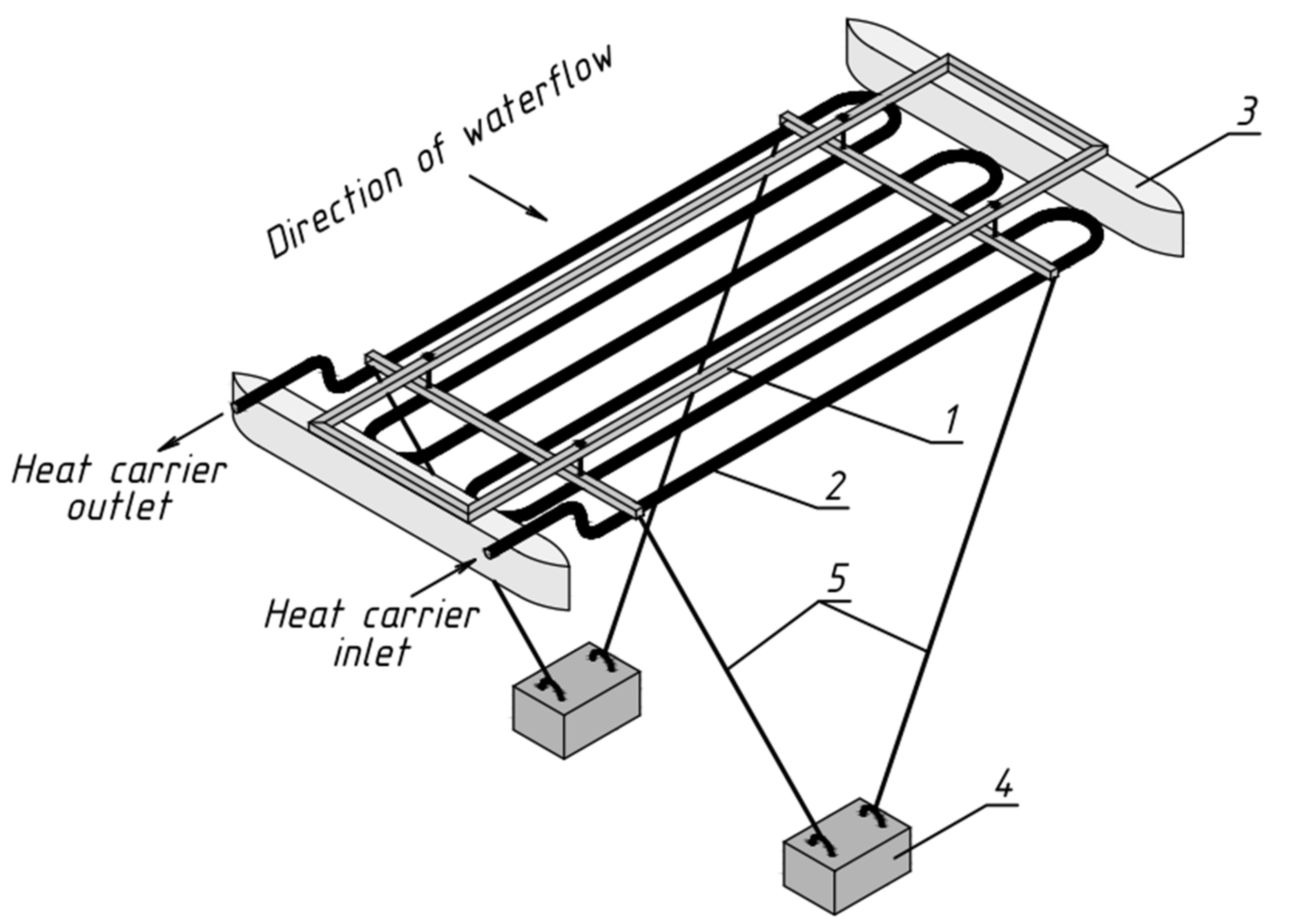
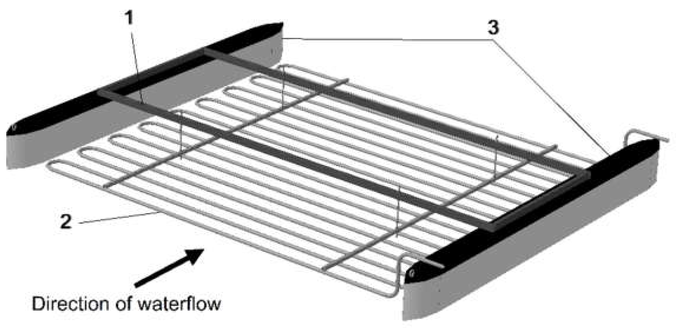
In this case, it is necessary to provide the monitoring of extracted low-grade heat flux by means of temperature sensors at the heat carrier inlet and outlet of the evaporator as well as heat carrier flow sensor.
In addition to the sensors for calculating power, heat fluxes, and COP, for more deep analysis of HPIs operation, sensors in the freon circuit of a heat pump, sensors for air temperature and other media, as well as some others, are also required. It was decided not to use expensive freon pressure sensors in the monitoring system, since in most cases the information about the temperature of freon is sufficient.
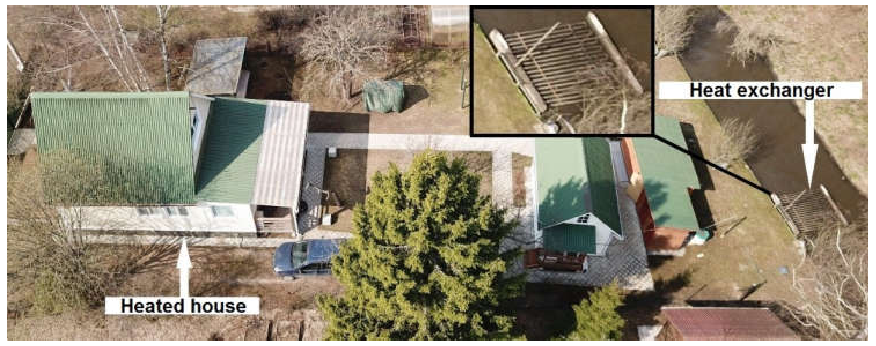
The monitoring system is organized to analyze the operation of the described water-to-air HPI based on an inverter heat pump using low-grade heat of the watercourse. Recall that in such an installation there is an intermediate heat carrier circuit for low-grade heat extraction, and the generated heat is transferred directly to the air. For such a case, the following set of parameters is determined, the measurement of which the monitoring system is supposed to provide:
-
temperature of a low-grade heat source (water in a watercourse);
-
temperature of the heat carrier at the entrance to the low-grade heat extraction site (at the entrance to the submersible heat exchanger);
-
temperature of the heat carrier at the outlet of the low-grade heat extraction site (at the outlet of the submersible heat exchanger);
-
temperature of the heat carrier at the inlet to the heat pump evaporator;
-
heat carrier temperature at the outlet of the heat pump evaporator;
-
heat carrier flow rate;
-
temperature of freon at the entrance to the evaporator;
-
temperature of freon at the outlet of the evaporator;
-
temperature of freon at the inlet to the condenser;
-
temperature of freon at the outlet of the condenser;
-
air temperature at the inlet to the condenser;
-
air temperature at the outlet of the condenser;
-
electric power consumed by the heat pump;
-
rotational speed of the inverter heat pump compressor.
Temperature sensors near the submersible heat exchanger and in a watercourse are needed to assess the efficiency of the heat exchanger. Information about the freon temperature at the evaporator inlet and outlet is necessary to determine the evaporation temperature and to control the completeness of evaporation. Air and freon temperature sensors near the condenser are required to account for the effects of room air temperature and condensation temperature. In other cases, depending on the complexity of the research task, the number of sensors can be both smaller and larger.
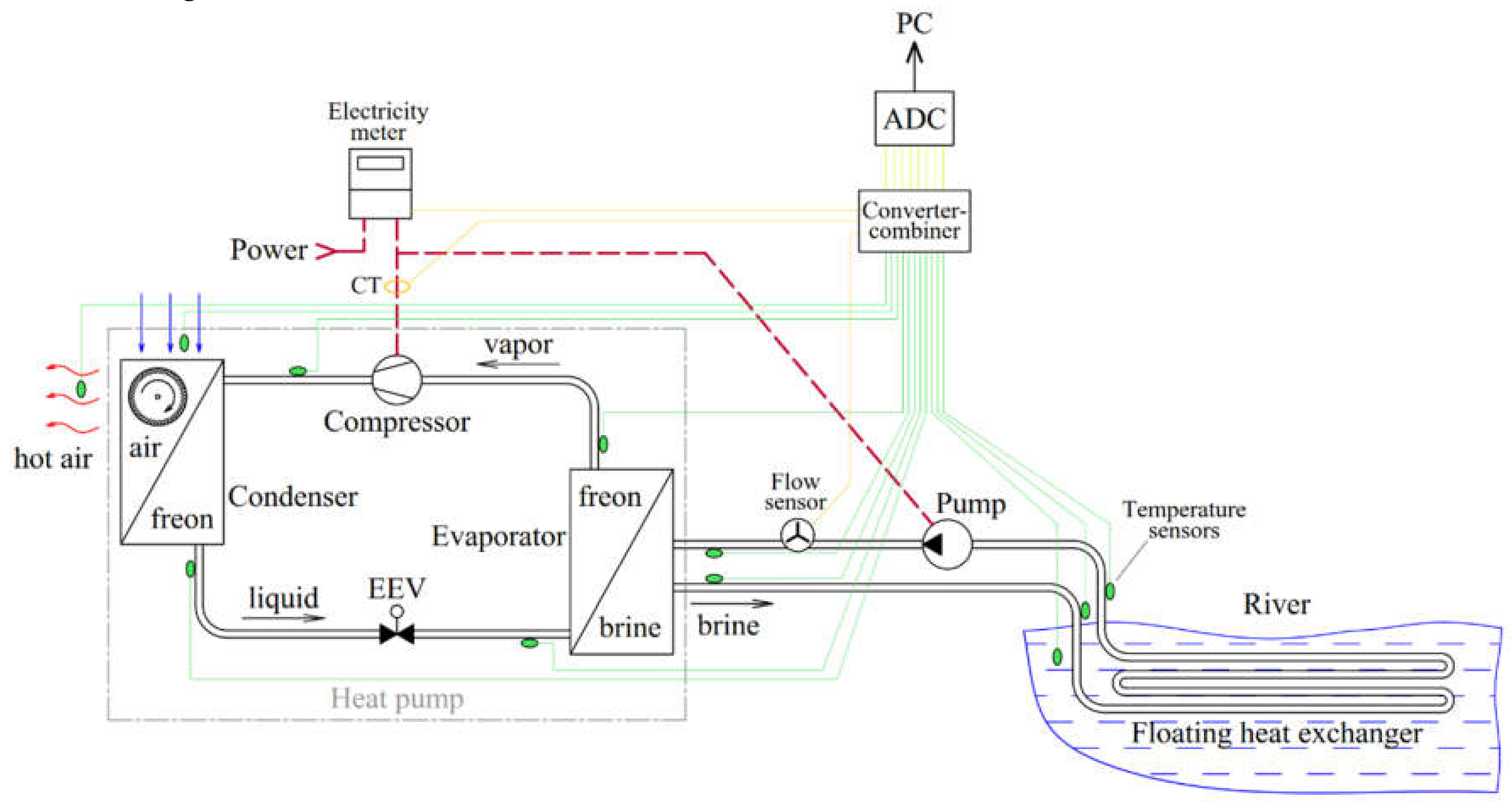
In Figure 4 schematic diagram of the HPI and the monitoring system with the location of the sensors are given.
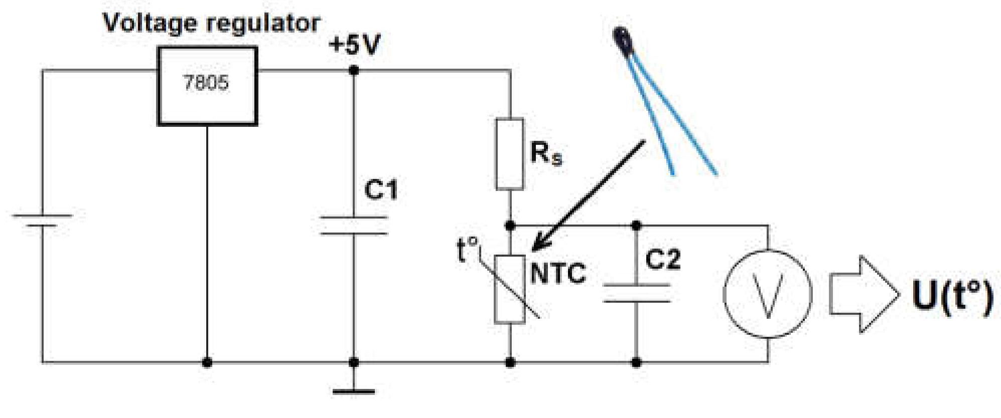
The temperature is measured using thermistors connected according to the scheme of the resistive voltage divider shown in Figure 5.
The capacitor C2 is needed for filtering impulse interference and is installed in the immediate vicinity of the ADC input, as significant interference can occur on long connecting wires, especially on unshielded ones. The optimum capacitance should be selected on a case-by-case basis. A capacitor with a large capacity filters out interference well, but the system’s response to temperature changes slows down.
In our monitoring system, we use high-precision NTC thermistors of the B57861-S/B57871-S type with a resistance of 10 kOhms with a tolerance of 1%. The high accuracy of temperature measurement is especially important when calculating the heat flux supplied to or removed from the heat carrier. So, in the case of using a heat carrier with a heat capacity of 3000 W/m∙K at a flow rate of 0.2 kg/s, every 0.1 K of the difference in the temperature of the inlet and outlet of the heat carrier corresponds to supplied or removed heat flux of 60 W. It is possible to achieve a sufficiently high accuracy of measuring these indicators in the system: the temperature difference between the readings of the sensors at the inlet and outlet of the heat exchanger during calibration process without heat transfer is kept below 0.05 K (generally 0.01–0.02 K).
The relatively high resistance of the selected thermistors (instead of the often used metallic thermoresistor with resistances of the order of 100 Ohms) allows us to provide sufficient accuracy in measuring the air temperature without significantly affecting the heating of the thermistor from the current flowing through it, since at the same applied voltage the heat release is inversely proportional to the resistance. So, at a temperature of 25 °C, the resistance of the thermistor of the selected type is 10 kOhm, the voltage on it in the used circuit with a voltage divider is eventually set to 0.45 V, and the heat generation according to Joule-Lenz law is:
Q = U 2 R = 0.45 2 10,000 = 2 × 10 5 W .
In addition, such high resistances significantly exceed the resistance of the connection wires. This allows the use of a two-wire sensor instead of a four-wire sensor connection (two wires for current supply and two for voltage drop measurement) without significant influence of wire resistance on measurement accuracy.
Parameters characterizing the intensity of the processes, such as electric power, mass or volumetric flow rate of substances and rotor speed, are usually measured by devices that output a pulsed or frequency signal with a characteristic frequency proportional to the measured value. Wattmeters and meters for measuring electrical energy in most cases have galvanically isolated pulse outputs through an optotransistor with a period between short-term pulses inversely proportional to the measured electrical power.
The fluid flow sensors YF-S201 used in the system for measuring the flow of heat carrier are impellers with an annular magnet rotating near the Hall sensor. Such a flow sensor is characterized by a low price, but requires preliminary calibration using trusted measuring instruments (accuracy ±5%). The sensor gives an output square-shaped frequency signal with a frequency proportional to the flow rate.
In an HPI with an inverter-type heat pump, it is required to register the compressor speed. To do this, it is enough to measure the frequency of the current on the compressor power line, for which a current transformer (CT) installed on one of the compressor power wires is used.
Both described sensors in the system under consideration give an output of a frequency signal with frequencies of the order of 20–200 Hz. In addition, sensors with a higher frequency signal can be included in the system. For example, our system temporarily used a signal from a fan motor feedback output with a frequency of up to 440 Hz. A simple ADC, unlike some microcontrollers, does not have a hardware interrupt function, i.e., cannot instantly record the moment of a sharp change in input voltage (arrival or completion of a pulse), but can only measure input voltage with a given frequency. Therefore, a significantly higher sampling frequency of the inputs (several times larger than the maximum signal frequency) is required in order to minimize the delay between the change in the input voltage and the moment of its measurement. The high frequency of measurements will create an excess data stream and create a significant load on the computer. In this regard such signals must be converted at first.
From this point of view, pulsed signals are preferable, upon registration of which it is sufficient to determine only the time interval between relatively rare pulses. In this case, the absolute value of the voltage on the channel does not play a role, therefore, it is irrational to allocate a separate ADC channel only for registering pulse signals from one sensor. In addition, the incoming pulses can be very short-lived: their duration can be changed by means of simple circuitry and reduced down to the minimum recorded ADC values.
Short-term pulses arriving at intervals measured in seconds can in some way be applied to the ADC inputs used to measure slowly varying absolute values of voltage from other non-pulse sensors (for example, temperature) and can be extracted using a program algorithm without any significant effect on the readings obtained with non-pulse sensor.
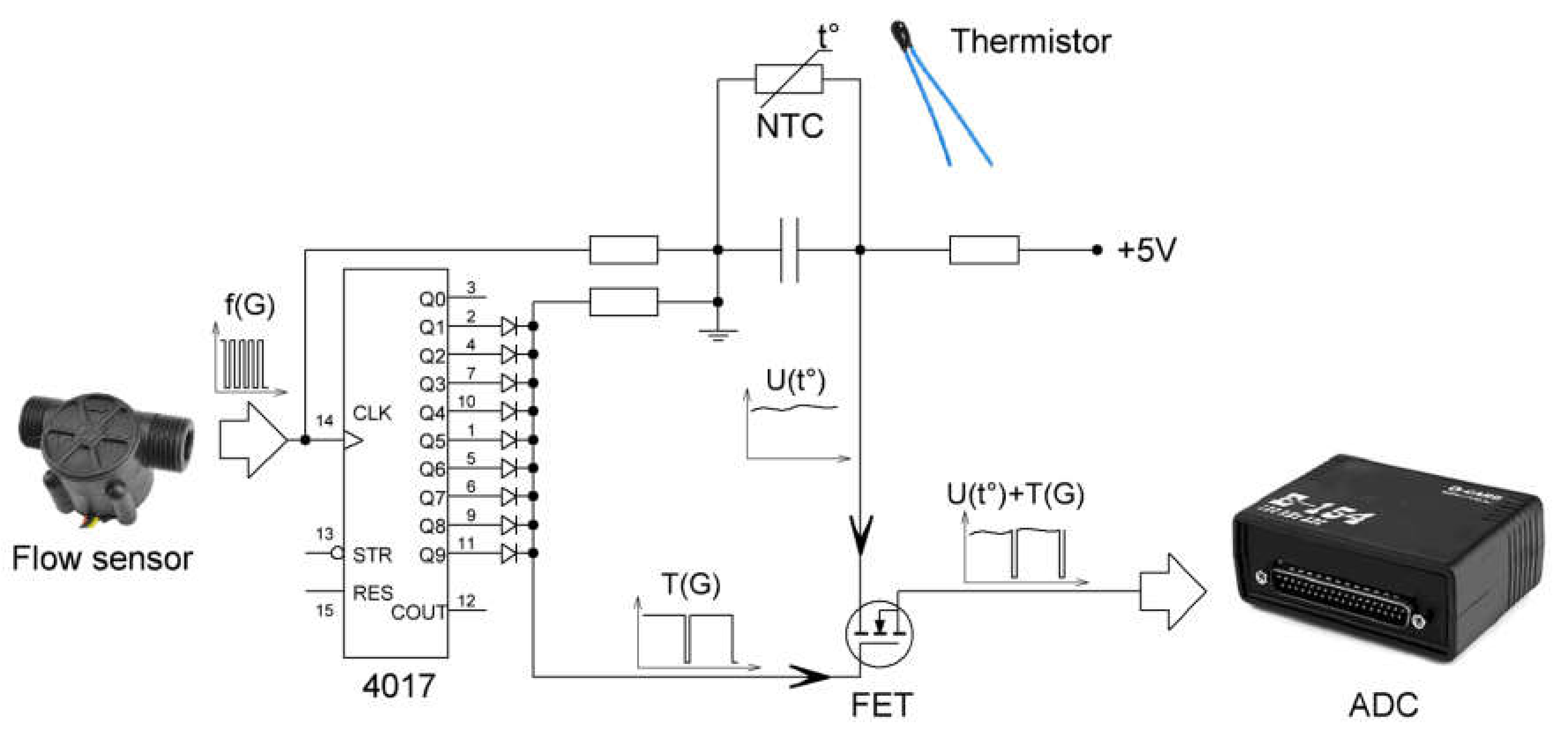
In connection with the described advantages of pulse signals, it was decided to convert the obtained frequency signals (from flow sensors, compressor speed sensor, etc.) to pulse ones. For this purpose, converters based on integrated counters/frequency dividers 4017 (CD4017/HCF4017) are assembled. The chip mentioned above allows you to divide the frequency of the original signal by 10 and change the duty cycle to 0.1. Depending on the frequency of the source signal, one-, two- or three-stage converters can be organized on this chip.
The scheme of sensors connection to one ADC input is shown in Figure 6.
A high-level signal arriving during the pulse causes a voltage drop across the gate of the field-effect transistor (FET), through which a signal is supplied from a non-pulse sensor (thermistor, in this case). As a result, the transistor closes, and due to the characteristics of the selected FET at the drain and, accordingly, at the input of the ADC, a sharp drop in voltage occurs, which is subsequently detected by the plugin as a new pulse. Subsequent software signal processing does not take into account the short-term absence of the signal from the thermistor in the temperature readings. Instead, the last recorded readings are displayed.
In the intervals between pulses, the voltage at the gate is restored, the transistor comes in the open state and the voltage from the thermistor is supplied to the ADC input. Given the almost complete absence of the current through the ADC inputs and, accordingly, the transistor, the open channel resistance of the transistor does not affect the measurement. The use of transistors with an isolated gate ensures that the gate voltage does not affect the voltage at the ADC input.
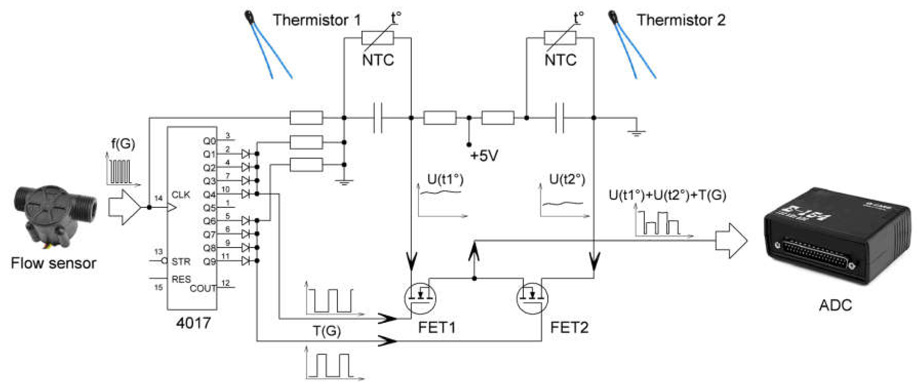
In order to be able to connect a larger number of sensors to a limited number of ADC inputs, a suitable circuit is developed. It has alternating supply of signals from several non-pulse sensors to one ADC input with separation by pulses from a 4017 chip, which converts the signal from a sensor with a frequency output. In this scheme, each non-pulse sensor is connected to the ADC input through a separate FET, the gates of which are connected to different groups of joint chip outputs (Figure 7).
In practice, the implementation of such a circuit with more than two non-pulse sensors connected to one ADC input causes difficulties, since it is problematic to process the combined signal from such a circuit to compare individual signals with specific sensors. In addition, the duration of registration of a signal from each non-pulse sensor is significantly less than the time of absence of a signal from an individual sensor. Therefore, it is possible to connect a maximum of two non-pulse sensors, the signals from which are alternated and separated by pulses from the 4017 chip.
To avoid false triggering of the counter, it is necessary to filter out impulse noise in the signal from a sensor with pulse output. A simple RC-filter (resistor + capacitor) is used for this purpose. In Figure 6 and Figure 7 filter elements at the input of the 4017 chip are not shown.

2.3. Monitoring System: Software

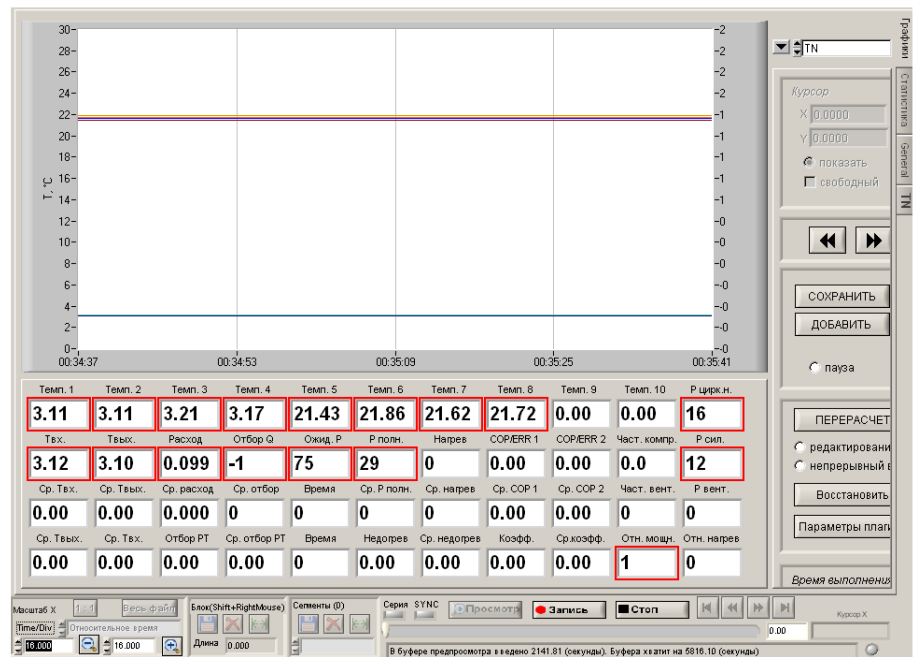
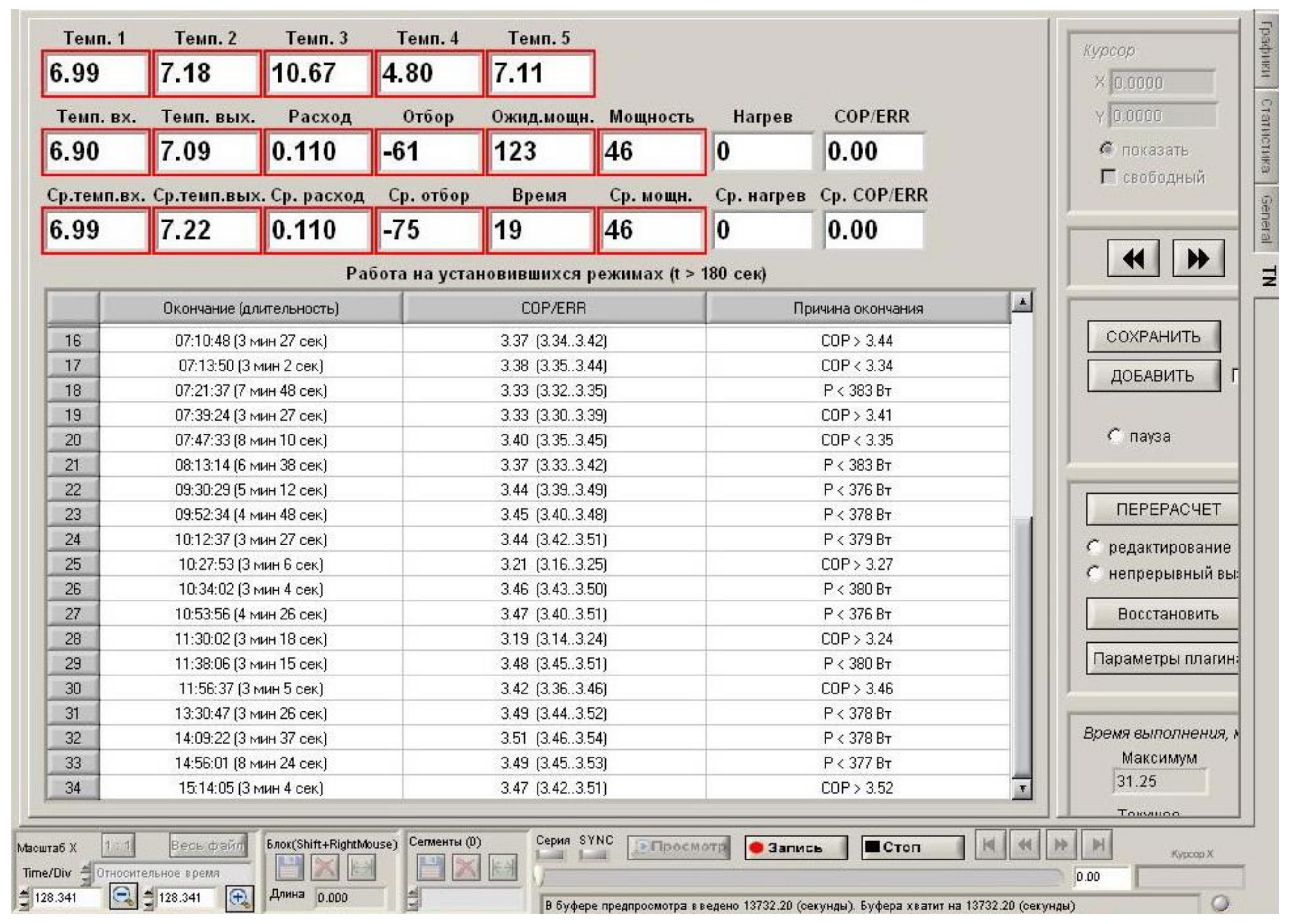
The plugin window in the process of monitoring the parameters of the HPI operation in two forms (in the mode of displaying temperature graphs and in the mode of displaying the table of registered steady-state operating modes) is shown in Figure 8 and Figure 9. The window in real time displays all the measured and calculated parameters of the HPI.
Incoming digitized readings from temperature sensors initially pass software interference filtering. The Kalman filter algorithm is used for this purpose.
The main task of the plugin is to process signals from various sensors to obtain measured values. The signal from the temperature sensors is the voltage on the thermistor, which is a part of the voltage divider. Based on the obtained voltage value, the resistance of the thermistor is calculated, after which the temperature is determined based on the temperature-resistance dependence known for the thermistor. Thermistor characteristic is usually provided by manufacturer in form of table. To be used in the calculation, it must first be converted to a function T R . The Steinhart–Hart equation is used for this purpose:
1 T = A + B · ln R + C · ln R 3 ,
where A , B and C are the coefficients, R is the thermistor resistance at temperature T (K). Coefficients are determined by solving a system of three equations for any three table points in the temperature region of interest. For used thermistors B57861-S/B57871-S, coefficients for the region of 258–343 K (−15–70 °C) are determined and the following relationship is obtained:
T R N T C = 1 2.774 E 3 + 2.502 E 4 · ln R N T C + 3.392 E 7 · ln R N T C 3 ,
where R N T C is the thermistor resistance, kOhm. Approximation accuracy for region 258—343 K: σ = 0.052 , R 2 = 99.8 .
Based on connection diagram (Figure 5) thermistor resistance can be calculated by the following formula:
R N T C = R S · U U 0 U ,
where R N T C is the resistance of the thermistor, R S is the resistance of the paired resistor in the voltage divider, U is the measured voltage and U 0 is the reference voltage (4.95 V).
Functions are directly entered into the plugin code. If various types of thermistors with different characteristics are used in the system, it is stipulated the possibility to add many dependencies to the plugin code, followed by selecting the necessary dependencies in the settings of individual sensors.
In the case of signals from sensors with a pulse output, in order to calculate the value of the measured parameter, it is necessary to measure the time interval between the arrivals of the pulses and to determine the desired value using the dependence entered in advance for a particular type of sensor. The same is applied to sensors with a frequency output, the signal from which is converted to a pulse using converters on 4017 chip. In this case, the division (thinning) coefficients of the converter for a particular sensor are taken into account.
However, since the allocation of a separate ADC channel for a pulse channel only is irrational, the plugin considers a circuit with the supply of pulse signals to the inputs involved in measuring absolute voltage values from non-pulse sensors. The possibility of processing combined signals for two options for joint connection to one ADC input is implemented:
-
one non-pulse sensor and one meter with a pulse output, or with a frequency output and connection through a converter on a 4017 chip;
-
two non-pulse sensors and one meter with a frequency output, connected through a converter on the 4017 chip.
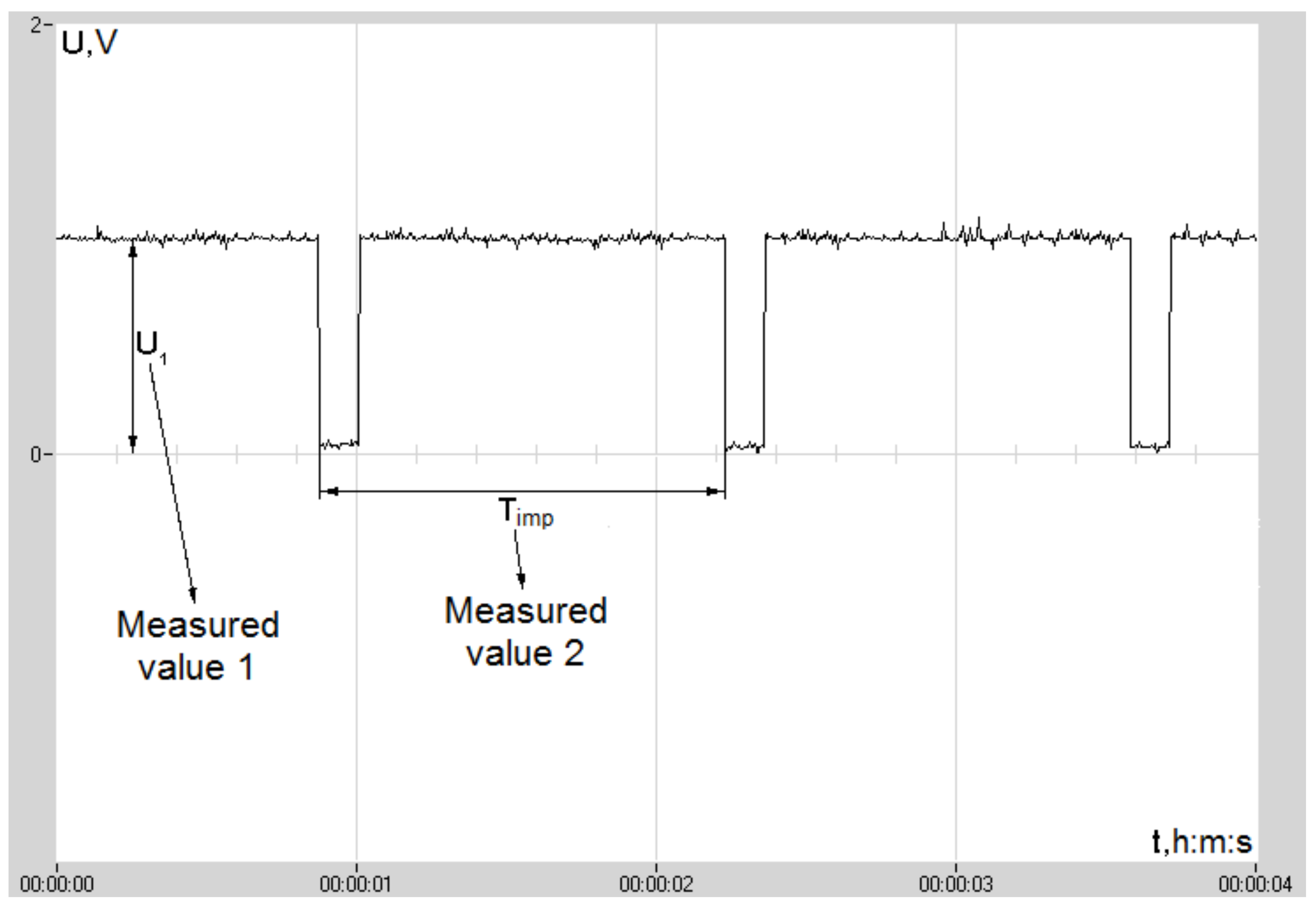
With the described scheme of sensors’ joint connection, pulse signals from the corresponding sensors, as well as frequency signals after their conversion to pulse, are recorded by the ADC as voltage dips at the inputs of a certain duration (Figure 10).
Over the duration of the pulse, which is usually from several tens to several hundred milliseconds, it is impossible to measure the value from a temperature or other non-pulse sensor connected to the same ADC input. However, taking into account the low rate of change of the analog values measured on the corresponding channels (it is recommended to send signals from temperature sensors to the considered channels, since the signal from them cannot change quickly), the analog value cannot change significantly for the indicated fractions of a second of signal absence. In this regard, during the pulse, until the voltage is restored from the non-pulse sensor, for display on the screen and in the file, as well as for calculating the values of other parameters, the last measured analog value is used.
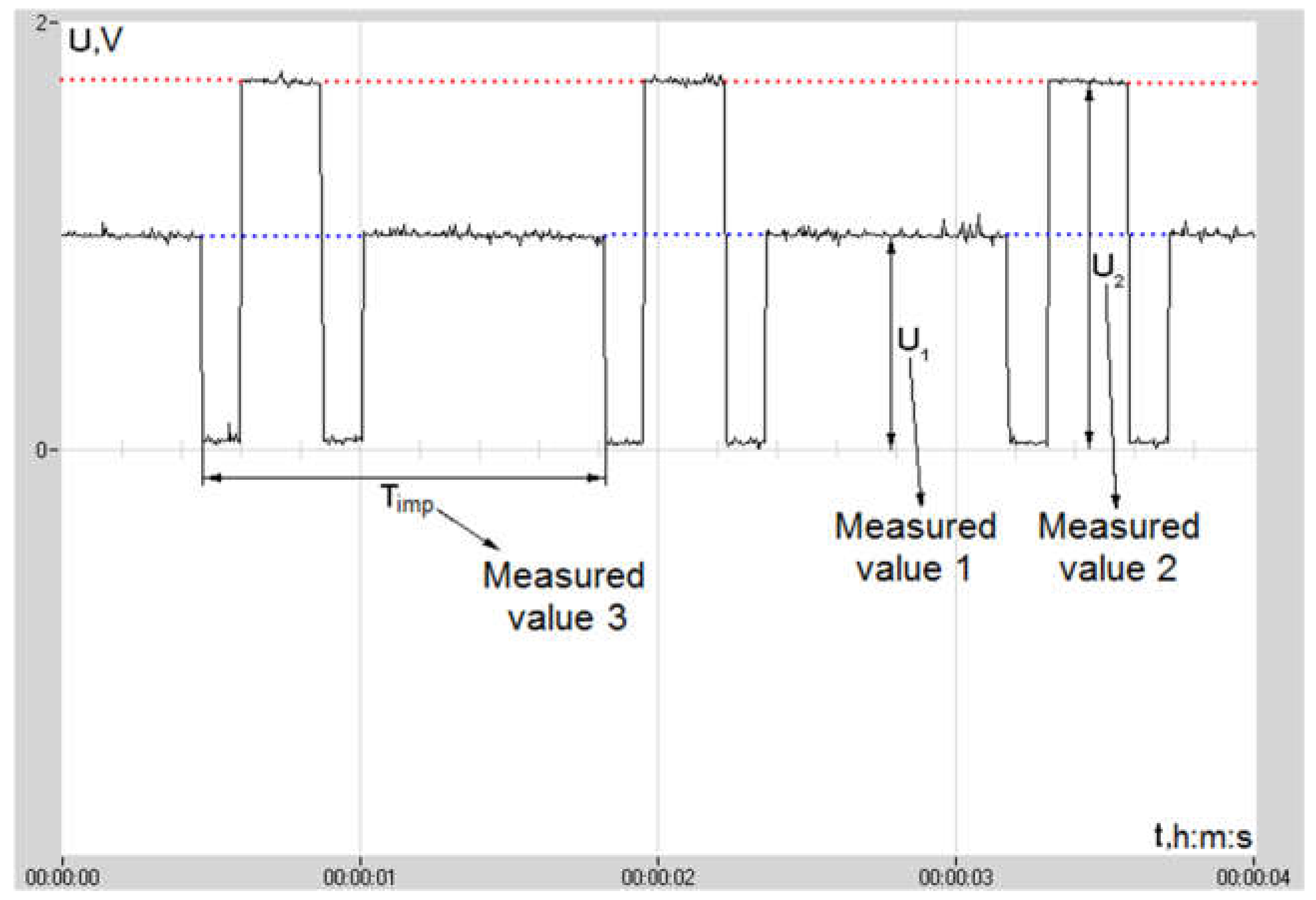
In the case of applying rolling signals from two non-pulse sensors to one ADC input, as in the previous case, the pulses are recorded by the ADC as voltage dips at the inputs of a certain duration. The duration of the signals from the first and second the non-pulse sensor may vary depending on the choice of outputs of the counter chip, from which the separation pulses are taken. When calculating the pulse value, the full period is taken into account, that is, the interval between every second pulse (Figure 11).
The principle of operation of the processing algorithms is similar in both cases, however, in the case of two non-pulse sensors, the algorithm is organized in a more complex way due to the need to identify and compare alternating signals from two different non-pulse sensors. A higher-level analog signal is detected and attributed to the sensor, the signal from which must obviously be higher, and a lower-level signal is respectively attributed to another sensor. Wherein, the last value recorded before the arrival of the separation pulse is stored and used to display on the screen and to the file, as well as to calculate the values of other parameters throughout the time the signal from the corresponding sensor is absent.
In addition, in the plugin it is implemented an algorithm for diagnosing steady-state heat pump operation modes. HPI with an extended intermediate heat carrier circuit and a large volume of heat carrier in it has a significant inertia and any targeted change in an initial parameter or an operator-independent significant change in conditions is accompanied by a long (from several minutes to tens of minutes) transient process, in most cases not representing interest for analysis. To study the influence of various parameters on the installation efficiency, it is required to determine the average performance and efficiency indicators over the long-term steady-state operation modes, accompanied by only a slight fluctuation in the values.
In this regard, it was important to ensure that the monitoring system automatically with accordance to the set criteria identified such established operating modes and collected data on them in a separate table (file).
The algorithm monitors changes in the following parameters:
-
temperature of the inlet and outlet of the heat carrier in the heat exchanger-evaporator;
-
heat carrier flow rate;
-
compressor rotation speed;
-
electric power;
-
COP.
For each of these parameters, the values of possible deviations are set in the plugin code. A steady-state operation mode is considered to be such a period of operation of the installation during which none of the specified parameters goes beyond the set tolerances of the deviation and the duration of which is not less than the value specified in the settings.
During the steady-state operation mode, the average values of all parameters are calculated. The accumulated data for the periods of steady operation (average values of the parameters and the duration of the mode) are recorded in a separate file. In addition, the duration of the mode, the average value of COP over it, and the reason for the end of the steady state are displayed as a table row in the plugin window.

2.4. Method of Measurement Efficiency of the Submersible Heat Exchanger

One of the main objects of study during the experiments was the submersible heat exchanger. The specific heat transfer coefficient was used to estimate intensity of heat exchange between water and heat carrier. The values of this coefficient need to be known in order to determine the optimal size of the heat exchanger in each particular case, and also it allows to compare the efficiency of various designs of the heat exchanger and schemes of its placing in a channel.
Heat transfer coefficient K is the proportionality constant between the heat flux q and the thermodynamic driving force for the flow of heat, i.e., the temperature difference Δ T :
q = Q S = K · Δ T ,
where Q is the whole heat flow through the surface, S is the heat transfer surface area.
For heat exchangers with a temperature changing along the tubes, the logarithmic mean temperature difference (LMTD) must be used as the temperature difference Δ T . Taking into account the intensity of the flow, the water temperature T W in the river changes negligibly due to the influence of the heat exchanger and can be considered constant over the entire heat exchange area. Then LMTD is:
L M T D = Δ T max Δ T min ln Δ T max / Δ T min = T W T i n T W T o u t ln T W T i n / T W T o u t = T o u t T i n ln T W T i n / T W T o u t ,
where T i n and T o u t are temperatures of the heat carrier at the inlet and outlet of the submersible heat exchanger.
The value of the heat flow Q is calculated similarly (2). Thus, the formula for calculating the heat transfer coefficient is as follows:
K = Q S · L M T D = G M · C h c · T o u t T i n S · T o u t T i n ln T W T i n / T W T o u t = G M · C h c · ln T W T i n / T W T o u t S
where G M is the mass flow rate of the heat carrier, and where the heat transfer surface S was calculated on the average radius of heat exchanger tubes:
S = π · R i n + R o u t 2 2 · L ,
where L is the total length of heat exchanger tubes.
Therefore, to find the heat transfer coefficient, four parameters must be measured: T i n , T o u t , T W and G M . For this purpose, the plugin was implemented an algorithm for diagnosing steady-state heat exchanger operation modes, similar to the described algorithm for a heat pump. The algorithm calculates the average values of these four parameters and the heat transfer coefficient for long periods of steady-state operation.

3. Results

The described monitoring system made it possible to optimize the HPI operating on a base low-grade heat of the open watercourse. Many dependencies of the influence of different factors on the overall efficiency of the installation have been identified.
First of all, the values of water-brine heat transfer coefficients were obtained for a developed submersible heat exchanger at various conditions of placement of the heat exchanger in a channel (Figure 12), which largely determines the efficiency of the installation as a whole.
In the case of an inclined arrangement, an angle of 7 degrees is used, as this is the maximum possible angle in the shallow watercourse under consideration.
The oscillatory state was considered to study the possibility of miniaturization of the heat exchanger by strengthening the heat transfer. Forced oscillations increase turbulence and thereby increase heat exchange between water and tubes surface. A mechanism for bringing the heat exchanger into oscillatory motion could work including from energy of the river flow without using an external energy source.
In addition, measurements were made for the design position, but in case with reduced heat carrier flow rate (0.1 kg/s instead 0.2 kg/s) and in case of littering by debris and sediments after a long stay in water. The results of these measurements are shown in Figure 13. The results were obtained for the watercourse under consideration with an average flow speed 0.15 m/s.
As can be seen on the bar chart, in all cases with the arrangement of the heat exchanger near the watercourse surface, heat transfer intensity is much higher than with the bottom arrangement. That justifies the proposed design with floats. There are some increases in heat transfer coefficient in cases of inclined position and under forced oscillations, but this increase would not compensate for the associated shortcomings (increased likelihood of debris trapping in it and design complication).
In addition, it was found that in the case of using an inverter heat pump in a HPI, that is, with a variable compressor speed, it is possible to slightly increase the overall efficiency of the installation by introducing regulation of the performance of the circulation pumps of low-temperature and/or high-temperature circuits. It is advisable to reduce the performance of the circulation pumps approximately in proportion to the current performance of the heat pump when it is not running at full power, which should lead to a decrease in total energy consumption. This effect is not prevented by the reduced efficiency of the heat exchanger (like the one shown in Figure 13, bar 3), since heat load on the heat exchanger is also reduced.

4. Conclusions

A monitoring system of a heat pump installation for heating a rural house using low-grade heat from a surface watercourse is developed. A number of novel or seldom-used solutions have been used to develop the monitoring system. It is shown that modern semiconductor thermistors can replace commonly used platinum temperature sensors and thermocouples. A strategy for processing frequency output signals from sensors through an ADC and a way for reducing the number of required input channels are described.
The monitoring system was used to evaluate the operation of heat supply of the house located in the Moscow region of the Russian Federation. A small channel flowing in the immediate vicinity of the house was used as a source of low-grade heat in the installation. The use of the monitoring system makes it possible to collect, in particular, experimental data to estimate the efficiency of the heat exchanger.
The design operating mode in which submersible heat exchanger is placed horizontally near the surface of the watercourse is investigated. The efficiency of the heat exchanger is also analyzed with some other configurations and conditions. Positioning alternatives are at the bottom or in an inclined way. The heat exchanger behavior is also analyzed under forced oscillations, reduced heat carrier flow rate, and in the presence of litter. The heat exchange efficiency is estimated by the value of the specific heat transfer coefficient. According to the measurements, design operating mode appears to be the most worthwhile technical solution. Compared to this scheme, the case with location of the heat exchanger at the bottom, in sediments, corresponds to about 20 times lower heat transfer coefficient and requires the use of a huge heat exchanger to ensure the operation of the heat pump. Although positioning the heat exchanger at an angle to the flow slightly improves efficiency with respect to the horizontal position, the probability of debris trapping in it also increases. Measurements show that littering may cause some efficiency reduction which, however, is not critical for the functioning of the heating system. Putting the heat exchanger under forced oscillations provides an increase in the heat transfer coefficient. This increase, however, is not sufficient to compensate the additional costs created by more complicated designs for the introduction of special oscillating mechanisms.
Based on the experience gained in developing the monitoring system and the operation of the heat pump installation, it is planned to create a compact, simple and cheap microcontroller unit. This device will be able to analyze the efficiency and to control individual elements of the installation. It is meant for using with heat pump heating systems for private homeowners and other consumers. Work in this direction is already underway. The unit is looked to be versatile enough to equip it with heat pump heating systems of various configurations, including the ones with a liquid heat distribution circuit. The model is supposed to provide for the possibility of controlling circulation pumps and auxiliary devices. For instance, in cold winters, typical of Russia and other northern countries, additional functions are often required to prevent freezing and control auxiliary electric heaters.

Author Contributions

Conceptualization, V.K., A.S. and U.F.; methodology and software, A.S.; validation, U.F., P.L.D.A. and V.K.; investigation, V.K., A.S. and U.F.; resources, A.S. and U.F.; writing—original draft preparation, A.S. and V.K.; writing—review and editing, U.F., P.L.D.A. and V.K. All authors have read and agreed to the published version of the manuscript.

Funding

This research received no external funding.

Conflicts of Interest

The authors declare no conflict of interest.

References

  1. Chemekov, V.V.; Kharchenko, V.V. The heat supply system for a self-contained dwelling house on the basis of a heat pump and wind power installation. Therm. Eng. 2013, 60, 212–216. [Google Scholar] [CrossRef]
  2. Adomavicius, V.; Kharchenko, V.; Valickas, J.; Gusarov, V. RES-based microgrids for environmentally friendly energy supply in agriculture. In Proceedings of the 5th International Conference Trends in Agricultural Engineering, Prague, Czech Republic, 2–3 September 2013; Volume 2013, pp. 51–55. [Google Scholar]
  3. Gusarov, V.A.; Kharchenko, V.V.; Sychov, A.O.; Rakitov, S.A.; Yudayev, I.V. Avtonomnyye sistemy teplosnabzheniya na osnove teplovykh nasosov vozdukh-voda (Autonomous heat supply systems based on air-water heat pumps). Energetika i Avtomatika 2013, 3, 67–71. (In Russian) [Google Scholar]
  4. Rees, S.J. Horizontal and compact ground heat exchangers. In Advances in Ground-Source Heat Pump Systems; Woodhead Publishing: Cambridge, UK, 2016; pp. 225–246. [Google Scholar] [CrossRef]
  5. Sarbu, I.; Sebarchievici, C. Ground-Source Heat Pumps: Fundamentals, Experiments and Applications; Academic Press: Cambridge, MA, USA, 2015; pp. 71–126. [Google Scholar]
  6. Spitler, J.D.; Mitchell, M.S. Surface water heat pump systems. In Advances in Ground-Source Heat Pump Systems; Woodhead Publishing: Cambridge, UK, 2016; pp. 225–246. [Google Scholar] [CrossRef]
  7. Long, N.; Dong, J.; Yao, Y.; Shen, C.; Qv, D.; Zhang, X. A review of heat pump systems for heating and cooling of buildings in China in the last decade. Renew. Energy 2015, 84, 30–45. [Google Scholar] [CrossRef]
  8. Zhang, C.; Zhuang, Z.; Huang, L.; Li, X.; Li, G.; Sun, D. Application prospect analysis of the surface water source heat-pump in China. In Proceedings of the Sixth International Conference for Enhanced Building Operations, Shenzhen, China, 6–9 November 2006. [Google Scholar]
  9. Sychov, A.; Kharchenko, V.; Vasant, P.; Uzakov, G. Application of various computer tools for the optimization of the heat pump heating systems with extraction of low-grade heat from surface watercourses. In Intelligent Computing & Optimization. ICO 2018. Advances in Intelligent Systems and Computing; Vasant, P., Zelinka, I., Weber, G.W., Eds.; Springer: Berlin, Germany, 2018; Volume 866, pp. 310–319. [Google Scholar] [CrossRef]
  10. Xi, C.; Hongxing, Y.; Lin, L.; Jinggang, W.; Wei, L. Experimental studies on a ground coupled heat pump with solar thermal collectors for space heating. Energy 2011, 36, 5293–5300. [Google Scholar] [CrossRef]
  11. Urchueguía, J.F.; Zacarés, M.; Corberán, J.M.; Montero, A.; Martos, J.; Witte, H. Comparison between the energy performance of a ground coupled water to water heat pump system and an air to water heat pump system for heating and cooling in typical conditions of the European Mediterranean coast. Energy Convers. and Manag. 2008, 49, 2917–2923. [Google Scholar] [CrossRef]
  12. Postrioti, L.; Baldinelli, G.; Bianchi, F.; Buitoni, G.; Di Maria, F.; Asdrubali, F. An experimental setup for the analysis of an energy recovery system from wastewater for heat pumps in civil buildings. Appl. Therm. Eng. 2016, 102, 961–971. [Google Scholar] [CrossRef]
  13. Zheng, W.; Zhang, H.; You, S.; Ye, T. The thermal characteristics of a helical coil heat exchanger for seawater-source heat pump in cold winter. Procedia Eng. 2016, 146, 549–558. [Google Scholar] [CrossRef] [Green Version]
  14. Blanco, D.L.; Nagano, K.; Morimoto, M. Experimental study on a monovalent inverter-driven water-to-water heat pump with a desuperheater for low energy houses. Appl. Therm. Eng. 2013, 50, 826–836. [Google Scholar] [CrossRef] [Green Version]
  15. Zhao, Z.; Zhang, Y.; Mi, H.; Zhou, Y.; Zhang, Y. Experimental Research of a Water-Source Heat Pump Water Heater System. Energies 2018, 11, 1205. [Google Scholar] [CrossRef] [Green Version]
  16. Büyükalaca, O.; Ekinci, F.; Yılmaz, T. Experimental investigation of Seyhan River and dam lake as heat source–sink for a heat pump. Energy 2003, 28, 157–169. [Google Scholar] [CrossRef]
  17. Yu, J.; Zhang, H.; You, S. Heat transfer analysis and experimental verification of casted heat exchanger in non-icing and icing conditions in winter. Renew. Energy 2012, 41, 39–43. [Google Scholar] [CrossRef]
Figure 1. Originally proposed submersible floating water-brine heat exchanger design (1—frame, 2—coil-pipe, 3—floats, 4—anchors, 5—ropes.).
Jsan 09 00011 g001
Figure 2. Aerial view of a heated house and a watercourse with a heat exchanger taken by from a quadcopter.
Jsan 09 00011 g002
Figure 3. Developed design of the submersible floating water-brine heat exchanger for the heat pump heating system under consideration. 1—frame, 2—coil-pipe, 3—floats.
Jsan 09 00011 g003
Figure 4. Schematic diagram of heat pump installation (HPI) with monitoring system.
Jsan 09 00011 g004
Figure 5. Connection diagram for thermistors.
Jsan 09 00011 g005
Figure 6. Scheme of sensors connection to one analog-to-digital converter (ADC) input.
Jsan 09 00011 g006
Figure 7. Connection scheme of several sensors to one ADC input.
Jsan 09 00011 g007
Figure 8. Plugin window in the mode of displaying temperature graphs and numerical values of all parameters.
Jsan 09 00011 g008
Figure 9. Plugin window in the mode of displaying numerical values of parameters and a table of registered steady-state operating modes.
Jsan 09 00011 g009
Figure 10. Waveform of the signal from the input of the ADC, which simultaneously receives signals from one non-pulse sensor and a meter with a frequency output.
Jsan 09 00011 g010
Figure 11. Waveform of the signal from the input of the ADC, which simultaneously receives signals from two non-pulse sensors and a meter with a frequency output.
Jsan 09 00011 g011
Figure 12. Various operating conditions of a submersible heat exchanger during experiments
Jsan 09 00011 g012
Figure 13. Obtained values of the specific heat transfer coefficient for various operating conditions of a submersible heat exchanger
Jsan 09 00011 g013

