Article

Data-Interpretation Methodologies for Practical Asset-Management

1
Applied Computing and Mechanics Laboratory, School of Architecture, Civil and Environmental Engineering, Swiss Federal Institute of Technology, 1015 Lausanne, Switzerland
2
ETH Zurich, Future Cities Laboratory, Singapore-ETH Centre, 1 CREATE Way, CREATE Tower, Singapore 138602, Singapore
*
Author to whom correspondence should be addressed.
J. Sens. Actuator Netw. 2019, 8(2), 36; https://doi.org/10.3390/jsan8020036
Submission received: 23 April 2019 / Revised: 7 June 2019 / Accepted: 11 June 2019 / Published: 22 June 2019

Abstract

:
Monitoring and interpreting structural response using structural-identification methodologies improves understanding of civil-infrastructure behavior. New sensing devices and inexpensive computation has made model-based data interpretation feasible in engineering practice. Many data-interpretation methodologies, such as Bayesian model updating and residual minimization, involve strong assumptions regarding uncertainty conditions. While much research has been conducted on the scientific development of these methodologies and some research has evaluated the applicability of underlying assumptions, little research is available on the suitability of these methodologies to satisfy practical engineering challenges. For use in practice, data-interpretation methodologies need to be able, for example, to respond to changes in a transparent manner and provide accurate model updating at minimal additional cost. This facilitates incremental and iterative increases in understanding of structural behavior as more information becomes available. In this paper, three data-interpretation methodologies, Bayesian model updating, residual minimization and error-domain model falsification, are compared based on their ability to provide robust, accurate, engineer-friendly and computationally inexpensive model updating. Comparisons are made using two full-scale case studies for which multiple scenarios are considered, including incremental acquisition of information through measurements. Evaluation of these scenarios suggests that, compared with other data-interpretation methodologies, error-domain model falsification is able to incorporate, iteratively and transparently, incremental information gain to provide accurate model updating at low additional computational cost.

1. Introduction

Improving living conditions and a global trend in migration of population from rural to urban centers result in increasing demand for civil infrastructure [1]. However, most present-day infrastructure has been built in the second half of the twentieth century and is close to the end of its designed service life. The deficit between demand and supply has been estimated to be USD 1 trillion in 2014 [2] and is increasing. Replacement of all aging infrastructure is unsustainable. However, civil infrastructure are generally designed using conservative models and, thus, they may possess reserve capacity beyond code requirements [3,4]. For quantification of such reserve capacity, better understanding of structural behavior is needed. Thus, decision making regarding asset-management actions such as repair, retrofit and replacement, is enhanced [5].
Measurements of structural response can be interpreted using physics-based models in order to enhance understanding of structural behavior. Increased availability and reduced cost of sensing techniques [6,7] and computational tools [8] have made model-based data interpretation feasible. However, all models are idealizations of reality [9]. Conservative modeling assumptions lead to large uncertainty, with systematic and correlated errors at measurement locations [10]. Many researchers have studied uncertainties that affect interpretation of civil-infrastructure response [11,12,13]. Improvement in quantification of uncertainties can help improve accuracy of data interpretation.
Interpretation of measurements using a physics-based model is referred to as structural identification. Due to the presence of uncertainties, structural identification, which is an abductive task, is an ill-posed problem. Methodologies for solving such inverse problems have been studied by many researchers [14,15,16,17]. In practical applications, residual minimization (also called model calibration) is the most commonly used model-based measurement-interpretation method. For residual minimization, optimal values of parameters governing model behavior are estimated by minimizing the residual between model predictions and measurements [18]. Although popular among practicing engineers due to its simplicity, residual minimization may provide inaccurate results [19]. An assumption made by residual-minimization methods is that the difference between model predictions and measurements is governed only by the choice of parameters [20]. This implies that systematic bias between the approximate model and measurements is not taken into account during parameter estimation. In other words, the difference between model predictions and measurements is assumed to be distributed as zero-mean uncertainty forms [10,21,22,23].
Another methodology that has gathered much interest from the data-interpretation community is Bayesian model updating (BMU). Traditionally, BMU employs an independent zero-mean Gaussian likelihood function [24]. Model parameters, considered as probabilistic distributions are updated using this likelihood function. Model-parameter combinations that provide predictions whose error with measurements are low are attributed higher likelihood. Many developments over the traditional implementation of BMU have been made to account for the presence of model bias [25,26,27]. However, mis-evaluation of systematic bias and correlations leads to inaccurate estimation of model parameters [28,29,30,31,32].
Goulet and Smith [29] presented a multi-model data-interpretation methodology called error-domain model falsification (EDMF). In EDMF, model-parameter instances are falsified when their predictions are not compatible with measurements. Compatibility is determined based on falsification thresholds that are computed based on the uncertainties affecting identification of parameter values. Estimation of uncertainties involves information available from tests, guidelines and engineering heuristics. EDMF has been shown to provide more accurate identification and predictions compared with traditional BMU and residual minimization [29,30,31,32].
Data interpretation for asset management is an iterative task, with re-evaluations required as new information becomes available. New information can be: new measurements; change in uncertainty conditions; and new diagnostic information. Pasquier and Smith [33] presented an iterative sequence-free data-interpretation framework using EDMF and highlighted the iterative nature of data interpretation. A similar framework for post-earthquake assessment using EDMF was presented by Reuland et al. [34]. Zhang et al. [35] developed a data-interpretation tool that employs BMU with the goal of assisting asset managers. Except from these studies, most present day research in structural identification has focused on damage detection within a sequential framework [36]. In addition, no research is available that evaluates the usefulness of data-interpretation methodologies such as BMU and residual minimization within iterative frameworks to assist asset managers faced with real-world challenges. Model-based data-interpretation has the potential to enhance asset management strategies. These strategies have been developed by many researchers using, for example, multi-criteria decision making [37,38] and asset-performance metrics [39,40].
Application of model-based data-interpretation methodologies for full-scale structures presents challenges such as unidentifiability [41] and, above all, constraints on computational cost [42]. Structural identification of full-scale structures, unlike laboratory experiments, are affected by environmental conditions such as wind [43] and temperature [44]. Moreover, numerical models of full-scale structures are computationally expensive. Many researchers have suggested using efficient sampling methods to alleviate constraints on computational cost. Residual minimization has been implemented with optimization algorithms such as genetic algorithms [45], artificial bee colony optimization [46,47], particle swarm optimization [48] and ant colony optimization [49] to reduce computational cost. BMU has been implemented using Markov-Chain Monte Carlo (MCMC) sampling [50], transitional MCMC sampling [51], and evolutionary MCMC sampling [52]. EDMF has traditionally been implemented using grid sampling, which is computationally expensive [53]. Adaptive-sampling strategies such as radial-basis functions [54] and probabilistic global search optimization [55] have been implemented to improve sampling efficiency for EDMF. While use of these search methods decreases computational cost, their efficiency for use in an iterative framework for data-interpretation has not been studied.
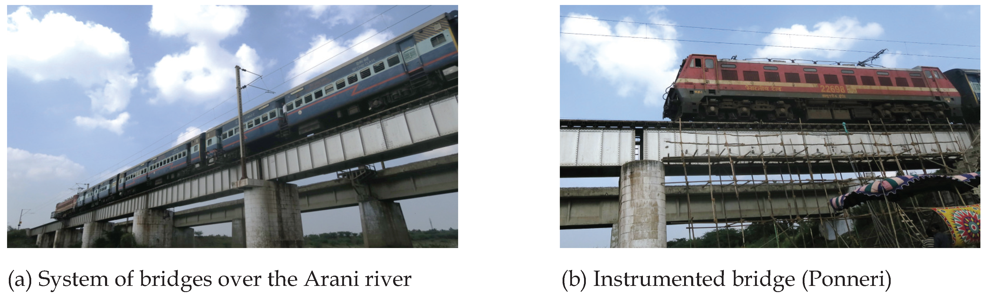
In this paper, several methodologies are compared based on their ability to efficiently incorporate new information and changing uncertainty definitions to provide accurate structural identification. Comparisons have been made using two full-scale bridge case studies to evaluate applicability of these data-interpretation methodologies outside of well-controlled laboratory environments.

2. Model-Based Data-Interpretation for Asset Management

Model-based data interpretation of civil infrastructure is difficult due to many scientific and practical challenges. To allow asset managers to exploit potential reserve capacity safely, accurate interpretation of measurement data is necessary. In addition, civil infrastructure (such as bridges and tunnels) form critical components in transportation networks. Their failure can cause loss of life and cascading disruptions to economies due to loss of connectivity. Thus, in addition to accuracy, ease of interpretation of data-interpretation results is imperative to asset managers.
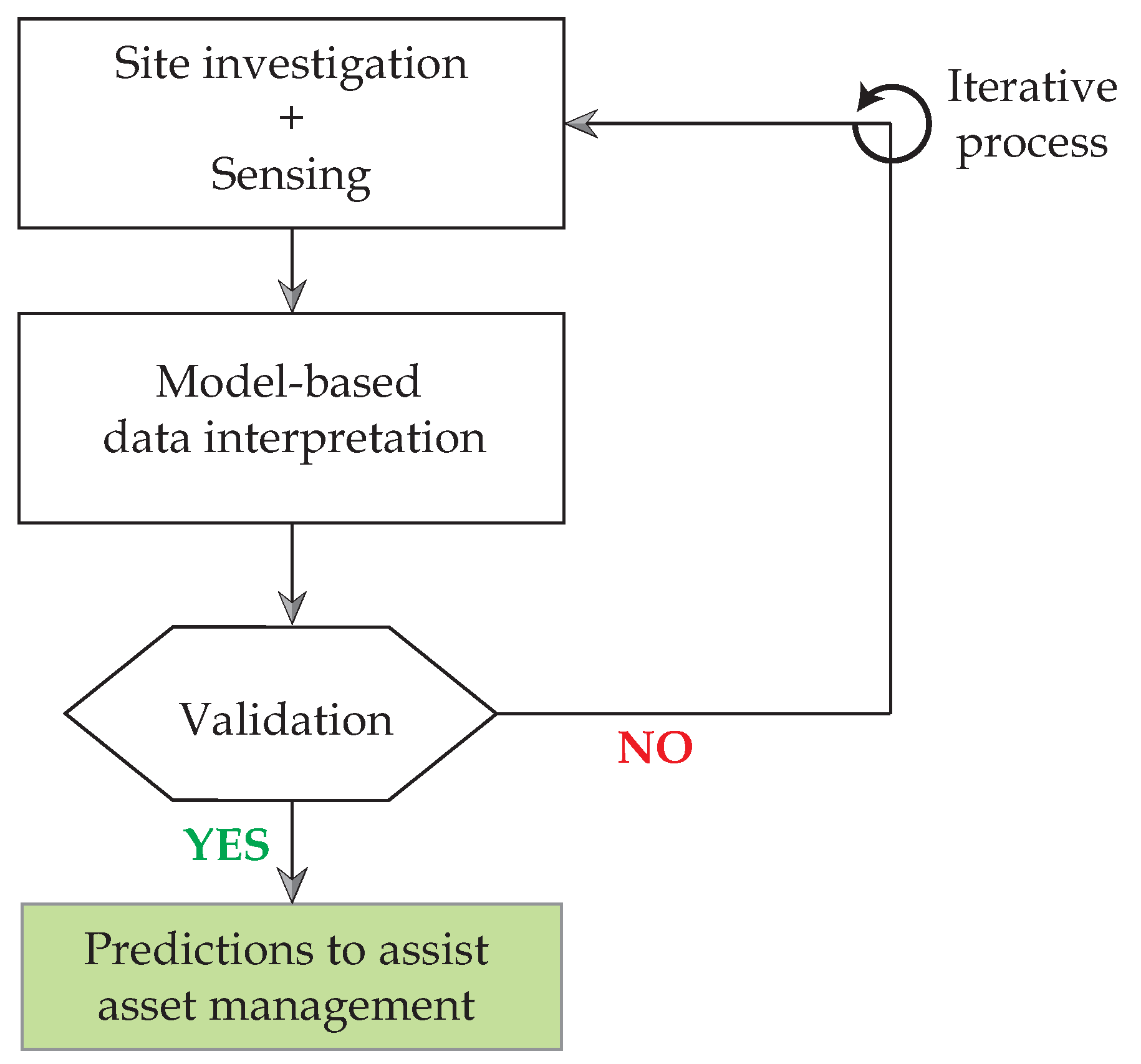
In Figure 1, typical steps involved in using model-based data-interpretation is presented. The sequence shown in the flowchart is general and a sequence-free framework for more specific asset management tasks was presented by Pasquier and Smith [33]. In this paper, the steps involving model-based data-interpretation and validation are discussed.
In Figure 1, site investigations help collect data useful for modeling and understanding sources of uncertainty. The task of sensing involves collecting data pertaining to structural response during either a load test or in-service conditions.
The task of model-based data-interpretation in Figure 1 consists of quantification of uncertainties, determination of a model class for identification and use of measurement data to update the values of parameters defined by the model class. Interpretation of measurement data may be carried out using various methodologies and some of these are described in Section 2.1.
A key task that is generally absent in most applications of model-based data interpretation is validation before making predictions. The validation task, subsequent to data interpretation (see Figure 1), has been recommended to be carried out using a leave-one-out cross-validation strategy in this paper. This is explained in Section 2.2.
Data interpretation, as shown in Figure 1, is iterative, especially as new information becomes available over the service life of the structure. New information takes the form of new measurements, improved understanding of uncertainties, improved understanding leading to a new model class, etc. Lack of validation of data-interpretation results may also necessitate iterations. Therefore, methodologies for data interpretation should be amenable to new information and flexible to changes.
In Section 2.1, data-interpretation methodologies that are available in the literature are described. These methodologies make implicit assumptions regarding estimation and quantification of uncertainties affecting structural identification. Methodologies also differ in the sampling strategies used to obtain appropriate solution(s). Accuracy of these methodologies in interpreting measurement data is dependant on the validity of assumptions. A leave-one-out cross-validation method to assess accuracy and precision of data-interpretation is explained in Section 2.2. In this paper, a comparison of data-interpretation methodologies based on iterative applications is presented. The objective of these comparisons and validation checks are to help engineers select a suitable methodology to interpret measurements using physics-based models.

2.1. Background of Data-Interpretation Methods

In this paper, four data-interpretation methodologies are compared with respect to their ability to provide accurate identification and incorporate new information in an iterative manner. In the following, the four methodologies are briefly introduced and their inherent assumptions are discussed.

2.1.1. Residual Minimization

In residual minimization, a structural model is calibrated by determining model-parameter values that minimize the error between model predictions and measurements. A typical objective function for residual minimization is shown in Equation (1).
θ ^ = argmin θ i = 1 n y g i ( θ ) - y i ^ ) y i ^ 2
In Equation (1), θ ^ is the optimum model-parameter set obtained using measurements and g i ( θ ) - y i ^ is the residual obtained between the model response, g i ( θ ) , and measurement, y i ^ , at measurement location i.
Predictions with models updated using residual minimization are limited to the domain of data used for calibration [56]. Therefore, calibrated model-parameter values may only be suitable for predictions that involve interpolation [56] and not for extrapolation (predictions outside the domain of data used for calibration) [19,20].

2.1.2. Traditional Bayesian Model Updating

Bayesian model updating (BMU) is a popular probabilistic data-interpretation methodology [24,57,58] based on Bayes’ theorem. In BMU, prior information of model parameters, P ( θ ) , is conditionally updated using a likelihood function P ( y θ ) to obtain a posterior distribution of model parameters, P ( θ y ) , as shown in Equation (2).
P ( θ y ) = P ( y θ ) · P ( θ ) P ( y )
In Equation (2), P ( y ) is the normalization constant. P ( θ ) is the prior distribution of model parameters, which indicates prior available knowledge regarding parameter values. The likelihood function, P ( y θ ) , is the probability of observing the measurement data, y, for a specific set of model-parameter values, θ . The most commonly used likelihood function is a L 2 -norm-based Gaussian probability-distribution function (PDF), as shown in Equation (3).
P ( y θ ) c o n s t a n t · exp - 1 2 g θ - y T Σ - 1 g θ - y
In Equation (3), Σ is a covariance matrix that consists of variances and correlation coefficients of uncertainties related to each measured location. In most applications of BMU, uncertainties at measurement locations are assumed to be independent zero-mean Gaussian distributions [59,60,61,62,63,64,65,66]. In addition, the variance in uncertainty, σ 2 , is assumed to be the same for all measurement locations. This leads the covariance matrix to be a diagonal matrix, with all non-zero terms being equal. However, the assumption of a L 2 -norm-based Gaussian distribution for uncertainty [67] and uncorrelated error [28] is rarely satisfied and may lead to a biased updated probability distribution [29,30,32].

2.1.3. Error-Domain Model Falsification

Error-domain model falsification (EDMF) is a data-interpretation methodology developed by Goulet and Smith [29]. EDMF is based on the assertion by Popper [68] that models cannot be validated by data; they can only be falsified. Model instances (instances of model-parameter values) are falsified based on information from measurements. Model instances that are not falsified form a candidate set, which is a subset of all possible parameter values based on the prior model parameter PDFs.
Generally, civil infrastructure are designed using conservative and simplified models. As a result, engineering models possess significant model bias from sources such as simplification of loading conditions, geometrical properties, material properties and boundary conditions. Extent of these uncertainties can only be estimated using engineering heuristics and usually takes the form of bounds.
Let ϵ m o d , q be the modeling uncertainty and ϵ m e a s , q the measurement uncertainty, both at a measurement location q. Let the structure be represented by a physics-based model, g ( θ ) . The true response of the structure at a measurement location is given by Equation (4).
y q + ϵ m e a s , q = R q = g q θ * + ϵ m o d , q
In Equation (4), g q θ * is the model response at a measurement location q for the real values of the model parameters, θ * . y q is the measured response of the structure at measurement location q. Rearranging the terms of Equation (4), a relationship among model response, g ( θ ) , measurement, y q , and uncertainties, ϵ m e a s , q and ϵ m o d , q , at location q is obtained, as shown by Equation (5).
g q θ * - y q = ϵ m e a s , q - ϵ m o d , q
In Equation (5), the residual between model response, g ( θ ) , and measurement, y q , at a sensor location, q, is equal to the combined model and measurement uncertainty. Engineers make design decisions based on predefined target reliability. Using the target reliability, ϕ , for identification, the criteria for falsification, thresholds T h i g h , q and T l o w , q , are computed using Equation (6).
ϕ 1 / m = T l o w , q T h i g h , q f U c , q ϵ c , q d ϵ c , q
In Equation (6), f U c , q ϵ c , q is the PDF of combined uncertainty at measurement location q and ϕ is the target reliability of identification. Thresholds, T h i g h , q and T l o w , q , correspond to the shortest interval providing a probability equal to target reliability, ϕ . In Equation (6), the term 1 / m is the Šidák correction [69], which accounts for m independent measurements used in identification of model parameters. In EDMF, compatibility of model predictions with measurements at each sensor location is considered as a hypothesis, which can have false positives and negatives. Inclusion of false positives as a candidate instance decreases precision of model updating, while falsely rejecting a model instance could potentially lead to falsification of true parameter values. Šidák correction controls the error rate such that the possibility of rejecting the true parameter values is lower than 1 - ϕ .
EDMF is traditionally carried out using grid sampling. In grid sampling, samples from prior distribution of model parameters, θ , are drawn. If n s samples are drawn from the prior distribution of each parameter, then these samples constitute a grid, which is called the initial model set (IMS). For n s samples drawn from n p parameters, the total number of model instances in the IMS is n s n p .
Residual between model responses, g ( θ ) , and measurements, y, are compared with the thresholds, T l o w , q and T h i g h , q . If the residual between model response and measurements lies within the thresholds for all measurement locations, then the model instance is accepted. This criteria for falsification is shown in Equation (7).
T l o w , q g q θ - y q T h i g h , q q 1 . . . m
If predictions for a model instance, θ i , does not satisfy Equation (7) for even one measurement location, then that model instance is falsified. All candidate model instances are considered equally likely and, thus, assigned a uniform probability density. Candidate models are used for making further predictions using the physics-based model with reduced parametric uncertainty [30]. The EDMF methodology has been applied to more than 20 full-scale systems since 1998 [4]. Recent applications include: model identification [70]; leak detection [71,72]; wind simulation [73]; fatigue life evaluation [74,75,76]; measurement-system design [77,78,79,80]; post-earthquake assessment [34,81]; damage localization in tensegrity structures [82]; and occupant localization [83].
EDMF when compared with BMU and residual minimization has been shown to provide accurate identification due to its robustness to correlation assumptions and explicit estimation of model bias based on engineering heuristics [29,30,31,32]. Although grid sampling carries some advantages with respect to practical applications and parallel computing, grid sampling remains computationally expensive [53].

2.1.4. Modified Bayesian Model Updating

To alleviate shortcomings of traditional BMU (see Section 2.1.2), a box-car likelihood function is utilized for modified BMU, which is more robust to incomplete knowledge of uncertainties and correlations than standard L 2 -norm-based Gaussian likelihood functions. The box-car likelihood function is developed using an L -norm-based Gaussian likelihood function [67], which is defined as shown in Equation (8).
L y θ = 1 / 2 σ for μ y - σ g ( θ ) - y μ y + σ , 0 otherwise .
In Equation (8), parameters of the likelihood function, μ y and σ , are determined using Equations (9) and (10).
μ y = T high + T low 2
σ = T high - μ y
In Equations (9) and (10), T low and T high are the thresholds computed for EDMF using Equation (6) for a target reliability of identification ϕ d . Modified BMU using such a box-car likelihood distribution has been shown to provide results similar to those obtained using EDMF [31,32].

2.2. Practical Challenges Associated with Model-Based Data Interpretation

As stated before, data interpretation is an iterative task that requires exploring results and re-evaluating results in light of new information regarding uncertainties or new measurements. In addition, the task of data-interpretation may have to be repeated when identification results are found to be inaccurate due to a wrong model class. Assessing accuracy is a challenge as knowledge of true parameter values is unavailable. Accuracy can be approximated with cross-validation methods [84]. While enabling accuracy estimation, such validation strategies are limited to the domain of data used for identification. Moreover, when these methods indicate that structural identification is inaccurate, diagnostics are required to re-assess the assumptions made during identification.
Cross validation of structural-identification results can be conducted using several techniques, such as leave-one-out, hold-out and k-fold. Hold-out and k-fold cross-validation require large measurement datasets for identification and validation. In structural identification of civil infrastructure, measurements are typically scarce with few sensors that provide information about structural behavior. Thus, leave-one-out cross-validation is preferred over other strategies for validating model-updating results.
In leave-one-out cross validation, observation from one sensor is omitted (left-out) and structural identification is carried out using all remaining measurements. Updated model-parameter values are then used to predict the model response at the omitted sensor. If the omitted measurement is compatible with updated model predictions, then structural identification is concluded to be accurate for that sensor location. This procedure is repeated by omitting each sensor separately in order to assess accuracy at all measurement locations.
Consider that n m measurements are acquired during a load test. These measurements are used for updating a physics-based model of the structure, g ( θ ) , which has parameters θ = [ θ 1 , θ 2 , . . . , θ n p ] , where n p is the number of parameters. Prior to model updating, the initial prediction at a sensor location j is given by Equation (11).
q j = g j θ + ϵ p r e d , j
In Equation (11), g j θ is the model prediction at sensor j for model parameters θ and ϵ p r e d , j is the model error from sources such as parameters not considered in the parameter vector θ , uncertainty in load and its position. The model-prediction distribution including model error before model updating is q j .
Let measurement from sensor j be excluded from model updating of parameters θ to perform leave-one-out cross-validation. The Sidâk correction for determining the threshold bounds, leaving one sensor out, is 1 n m - 1 . Model parameters, θ , are updated to obtain candidate model parameters, θ . Model updating is performed using the four methodologies described in the previous sections. The following equations apply directly to EDMF and modified BMU. For traditional BMU, they can be calculated based on the 95th-percentile bound of the prediction distribution. Updated parameters, θ , are provided as input to the physics-based model, g ( θ ) , to predict the model response at the omitted sensor, j, as shown in Equation (12).
q j = g j θ + ϵ p r e d , j
In Equation (12), q j is the distribution of updated model predictions at sensor location j. Depending on the uncertainties and relationships between model parameters and response, the prediction distributions obtained using Equations (11) and (12) are irregular. They are assumed to have uniform distributions based on the principle of maximum entropy. When bounds of the updated distribution of model predictions include the measured value, which has been left out for model updating, then identification is considered to be accurate.
Using leave-one-out cross validation, precision of structural identification can be quantified in addition to accuracy. Precision is a measure of variability either in updated model-parameter distributions or model predictions. Using leave-one-out cross-validation precision is estimated using the error between the updated model-prediction distributions and corresponding measurements. The model-prediction distribution at sensor j before and after model updating is given by Equations (11) and (12). The measurement at this sensor location is y j . The prediction error is the residual between model predictions and measurement. The prediction error distribution at sensor j, before and after model updating are uniform and their ranges are given by Equations (13) and (14).
R j = q j , m a x - q j , m i n y j
In Equations (13) and (14), R j and R j are ranges of prediction-error distributions relative to the measurement at sensor j before and after model updating. For n m cases of leave-one-out cross-validation, n m prediction-error ranges before and after model updating are obtained. Considering prediction-error ranges for all cases of leave-one-out cross-validation before and after model updating, the precision index, φ , is defined as shown in Equation (15).
φ = μ R - μ R μ R
In Equation (15), μ R and μ R are the mean of prediction-error ranges, before and after model updating, over all cases of sensors left out. Precision, φ , represents reduction in prediction error after model updating and ranges from 0 to 1. Precision, φ , equal to zero implies no gain in information from model updating. In such situations, μ R is equal to μ R , implying that on average over all cases of leave-one-out cross-validation, no reduction in prediction uncertainty is obtained. Precision index, φ , equal to one implies perfect model updating wherein updated parameter and consequently the prediction distributions have zero variability.

3. Full-Scale Applications

In this section, with the help of two full-scale case studies, the application of four data-interpretation methodologies is compared. Comparisons are made with respect to their ability to provide accurate identification and transparently and iteratively incorporate new information.

3.1. Ponneri Bridge

Ponneri Bridge, shown in Figure 2b, is a steel railway bridge located close to Chennai, India. It is part of a system of bridges (see Figure 2a) built in 1977 that comprises a railway crossing over the Arani river.
The behavior of each bridge in this system is independent of the others. One of the bridges in this system, referred to as Ponneri Bridge, is instrumented. This is the first bridge in the system for a train entering from Chennai and heading north. The bridge has a span of 18.3 m and is composed of two steel I-section girders, as shown in Figure 3. The two steel girders are connected through diagonal cross-bracing with a spacing of 1.6 m, which provides the bridge with stiffness in the transversal direction.
A finite-element (FE) model of the Ponneri Bridge was developed in Ansys [85]. In the model, the steel girders were modeled using SHELL182 elements. Diagonal bracings (see Figure 3) connecting the steel girders are modeled using BEAM188 elements. The bridge was modeled as simply supported with perfect pin-conditioned support at end B (see Figure 3a) and a partially pin-conditioned support at end A. At end A, the support was modeled to have infinite vertical stiffness with stiffness in longitudinal direction (along the span) parameterized using zero-length spring elements, COMBIN14 (roller support). The bounds of this parameter, K A , z , was estimated using the FE model and is reported in Table 1. Other than stiffness of support at end A in longitudinal direction, the Young’s modulus of steel, E s , was parameterized. The bounds for E s , reported in Table 1, were conservatively estimated based on the probabilistic model for modulus of elasticity of steel provided by Vrouwenvelder [86].
Using the FE model, strain measurements for the bridge were simulated at 16 locations, which are shown in Figure 4. Use of simulated measurements helped compare accuracy of model updating for various scenarios using four data-interpretation methodologies.
When simulating measurements using the FE model, model bias was introduced by assigning partial rotational rigidity to the boundary conditions at supports A and B. Other than the model bias introduced, the values of model parameters, E s and k A , z , assigned to simulate measurements for two conditions of the bridge are shown in Table 2.
The before-retrofit scenario in Table 2 is the present condition of the bridge. The bridge was then assumed to be retrofitted by replacement of bearing at support A. The new bearing prevents translational movement of the bridge, similar to the bridge bearing at support B. This was represented by increased stiffness of the support A in the longitudinal direction in Table 2. For the two scenarios reported in Table 2, measurements were simulated for a train passing over the bridge. The train was positioned on the bridge such that it produces maximum strain at sensors close to mid-span, as shown in Figure 4.
Using the two scenarios of the Ponneri Bridge (see Table 2), the applicability of four data-interpretation methodologies to provide accurate structural identification was compared. As measurements were simulated, knowledge of the “true” parameter values helps assess identification accuracy in the presence of systematic bias.
Identification of parameters, E s and K A , z , had to be carried out in the presence of uncertainty from multiple sources, such as model bias (due to partial rotational stiffness of end conditions) and sensor noise (added to measurements). Estimations of these uncertainties are shown in Table 3.
The two sources of uncertainties shown in Table 3 were combined using Monte Carlo sampling to determine the updating criteria for traditional BMU, modified BMU and EDMF. For traditional BMU, a zero-mean L 2 -norm-based Gaussian likelihood function as defined by Equation (3) was developed. Falsification thresholds for EDMF were calculated using Equation (6). L -norm-based Gaussian likelihood function for modified BMU was developed using Equations (8)–(10). Using the Ponneri case study, the four data-interpretation methodologies were compared with respect to their ability to provide accurate structural identification as well as their amenability to incorporate changes in uncertainty definitions with respect to four identification scenarios, as shown in Table 4.

3.1.1. Scenario 1: Structural Identification before Retrofit, Ignoring Model Bias

Structural identification of E s and k A , z was conducted with measurements recorded before retrofit of the Ponneri Bridge. The first iteration of data interpretation was carried out without taking into account model bias (Scenario 1 in Table 4).
For EDMF, an initial grid of model instances was generated based on the prior distribution of model parameters (see Table 1). A total of 273 model instances (13 k A , z instances multiplied by 21 E s instances drawn from the prior parameter distributions) were generated and provided as input to the FE model. Model instances whose responses were compatible with measurements at all sensor locations were accepted as part of the CMS. Falsification thresholds obtained by ignoring the model bias falsified all model instances. Thus, the model class is falsified. Falsification of the entire model class indicates mis-evaluation of uncertainties.
Modified BMU was conducted with a boxcar-shaped likelihood function (see Equation (8)). Samples from the joint posterior PDF of model parameters were drawn using MCMC sampling. The starting point was determined using MC sampling. Without taking the model bias into account in development of the likelihood function, after 1000 MC samples, no starting point was obtained, which suggests rejection of the model class by modified BMU, in a similar way to EDMF.
Traditional BMU was conducted with a zero-mean Gaussian likelihood function, without taking into account the model uncertainty. The posterior PDF thus obtained was precise and biased from the true parameter values used to simulate the measurements. Similar to traditional BMU, residual minimization returned parameter values, 215 GPa and 4.5 log N/mm, as optimal. These values were inaccurate and biased from the true parameter values (see Table 2).

3.1.2. Scenario 2: Structural Identification before Retrofit, Considering Model Bias

Based on diagnostics obtained using EDMF and modified BMU, data-interpretation was repeated by including model bias (Scenario 2 in Table 4). EDMF, with re-calculated falsification thresholds and without requiring any new simulations, provided the CMS shown in Figure 5a.
Modified BMU was repeated by taking into account the model bias. Due to limitations on computational cost in using a FE model of a full-scale bridge, only 500 samples were drawn using MCMC sampling. A scatter plot of the samples drawn from the joint posterior PDF of model parameters, E s and k A , z , is shown in Figure 5b.
Traditional BMU was also repeated with a zero-mean Gaussian likelihood function using MCMC sampling (500 samples). A scatter plot of the samples drawn is shown in Figure 5c.
In Figure 5, the values of parameters used to simulate measurements are also shown for comparison. For EDMF and modified BMU, the “true” parameter values lie within the updated values of model parameters obtained, as shown in Figure 5a,b. However, for traditional BMU, the updated posterior distribution of model parameters does not include the “true” parameter values (see Figure 5c). Therefore, EDMF and modified BMU provide accurate structural identification for the Ponneri Bridge before retrofit actions, while traditional BMU does not. Since uncertainties were ignored in residual minimization, it was not repeated for changes in estimation of uncertainties.

3.1.3. Scenario 3: Structural Identification after Retrofit, without Re-Evaluating Prior Parameter Distributions

Simulated measurements after retrofit were used for structural identification using the four data-interpretation methodologies (Scenario 3 in Table 4). Replacement of the bearing at support A increased the stiffness of the support in longitudinal direction. The parameter values used to simulate the bridge response (see Table 2) lie outside the bounds of the prior distribution of model parameter k A , z (see Table 1). Therefore, EDMF falsified the entire model class, which implies either uncertainty or other assumptions have to be re-evaluated. Similar to EDMF, modified BMU failed to find a starting point, which suggests that no parameter values from the prior distribution of model parameters have a non-zero likelihood.
Traditional BMU using MCMC sampling found a starting point and identified a posterior with low variability (high precision). As uncertainties affecting structural identification were not changed compared with Scenario 2, this precision was not due to decrease in uncertainty rather mis-evaluation of the prior distributions of model parameters, which have to be re-evaluated.
EDMF, in addition to falsifying the model class, provided diagnostics to re-assess the uncertainty definitions. A comparison of rejected model predictions at all sensor locations with falsification thresholds suggests that the prior distribution of model parameters have to be re-evaluated. Moreover, the error between model response and the thresholds is not the same at all sensor locations, suggesting a systematic source of uncertainty. The only systematic uncertainty source in the model class is K A , z and the prior distribution of this parameter was modified to be uniform with bounds [3, 8] log N/mm.

3.1.4. Scenario 4: Structural Identification after Retrofit, after Re-Evaluating Prior Parameter Distributions

Model parameters were identified with new prior distributions using the four data-interpretation methodologies. The updated parameter distributions obtained using the three probabilistic data-interpretation methodologies are shown in Figure 6 (Scenario 4 in Table 4).
In Figure 6, a scatter plot of samples from the updated parameter distributions is shown. Using post-retrofit measurements of the Ponneri Bridge, all three probabilistic data-interpretation methodologies provided accurate updated parameter distributions. Residual minimization provided 215 GPa and 7 log N/mm as optimal parameter values, which were biased from the “true” parameter values (see Table 2).
To summarize, EDMF and modified BMU provide accurate model updating for all scenarios, before and after retrofit (Cases 1–4 in Table 4). Traditional BMU (considering 95th percentile bounds) provided accurate identification only post-retrofit with appropriate estimation of priors (Case 4 in Table 4). Residual minimization did not provide accurate model updating for any scenario. The various data interpretation scenarios were typical iterations due to unsuccessful validation, as described in Figure 1.

3.1.5. Interpretation of Identification Results

Residual minimization is the most commonly used data-interpretation methodology in practice, due to the simplicity of updating criteria (calibration) and ease of result interpretation (single optimal values). However, residual minimization is unable to provide accurate model updating in presence of large modeling uncertainties. Probabilistic data-interpretation methodologies account for the presence of modeling uncertainties, thereby improving accuracy, sometimes at the cost of transparency in understanding model-updating results.
EDMF provides a set of candidate models that are compatible with measurements. Modified BMU provides a bounded joint posterior PDF. Thus, posterior obtained using modified BMU can also be interpreted as updated bounds on model parameters, similar to those obtained using EDMF. Traditional BMU using uniform priors and a L 2 -norm-based Gaussian likelihood function provides an informed (not uniform) joint PDF as posterior. The normality of the posterior PDF is dependent on the information gained from measurements. In Figure 7, a comparison of results obtained from model updating using the three probabilistic methodologies for parameter K A , z is shown.
In Figure 7a, updated bounds of the parameter K A , z obtained using EDMF are highlighted. Using these bounds, an engineer is able to interpret the structural behavior for making further predictions to assist asset-management. For example, the updated bounds in Figure 7a indicate that the boundary-condition stiffness (in longitudinal direction) is low, thus the engineer can assume the structure to have a roller support. With this assumption, an engineer is able to make predictions with appropriate additional uncertainty from updated parametric variability. Modified BMU also provides updated bounds of the parameter K A , z , as shown in Figure 7b.
Traditional BMU, unlike EDMF and modified BMU, provides an informed posterior PDF, as shown in Figure 7c, where the marginal posterior PDF of model parameter K A , z is highlighted. However, informed PDFs do not directly assist engineers in interpreting results with respect to their physical meaning. Post-processing of results, such as calculation of MAP or 95th-percentile bounds, is necessary for engineers to interpret the physical meaning of interpretation results. With such post-processing, the engineers can determine physical meaning of results obtained from model updating and subsequently use them to make further predictions. In addition, as shown in Figure 7, traditional BMU does not provide accurate identification of the parameter, K A , z . An updated understanding of structural behavior, provided as bounds, helps engineers decide upon model-parameter values to be chosen for further predictions in a transparent manner and also reduce computational cost.

3.1.6. Comparison of Computational Cost

While EDMF and modified BMU provide compatible model updating, EDMF with grid sampling is more efficient than modified BMU in incorporating changing uncertainty definitions, such as changes to combined uncertainty estimation and prior parameter distributions.
Grid-sampling based model instances for EDMF were simulated using parallel computing. For the pre-retrofit scenario (Scenario 1 in Table 4), a grid of 273 model instances (IMS) was discretized into four groups and each group was simulated with a different core. Predictions from model instances were evaluated for compatibility with measurements using EDMF to obtain a CMS. Pre-retrofit, the first estimate of uncertainty without including model bias (Scenario 1 in Table 4), falsified all 273 model instances. As discussed in Section 3.1.1, this provides diagnostics to re-evaluate uncertainties and include model bias. Including model bias (Scenario 2 in Table 4), 127 model instances from 273 model instances were accepted into the CMS (see Figure 5a). Post-retrofit, no model instance from the IMS were found to be compatible with the new set of measurements (Scenario 3 in Table 4). This provides diagnostics to re-evaluate the prior distribution of model parameter K A , z , as explained in Section 3.1.3. Due to change in prior distribution of model parameter K A , z , 168 new model instances were added to the IMS, as shown in Figure 8 (Scenario 4 in Table 4). Only the additional model instances were evaluated again to obtain a new CMS using EDMF. CMS after changing prior distribution of model parameter K A , z contains 40 model instances. Thus, using EDMF with grid sampling helps save significant computational cost when iterative evaluations of uncertainty conditions and prior distribution of model parameters are required.
Modified BMU and traditional BMU were carried out in this study using MCMC sampling without parallel computing. MCMC sampling and other adaptive sampling strategies utilize assumptions of the posterior form of the solution space to improve efficiency of sampling. However, changes to prior distributions or uncertainty estimations (likelihood function) alter the solution space and, thus, require a complete re-start. This significantly increases computational cost when data interpretation has to be carried out iteratively. A comparison of the cumulative computational cost incurred in applying these methodologies for multiple scenarios of identification is shown in Figure 9.
Figure 9 shows the cumulative computational cost incurred related to the three probabilistic data-interpretation methodologies. As EDMF with grid sampling does not require a complete re-start between iterations of identification and can be carried out using parallel computing, it incurs the lowest computational cost. Modified and traditional BMU incur much higher computational costs due to repeated re-starts that increase evaluations required using computationally expensive physics-based models.
A key aspect that is not included in Figure 9 is the computational cost incurred in appropriately carrying out MCMC sampling for modified and traditional BMU. For MCMC sampling, the computational cost depends upon user-defined step-sizes, which affect acceptance rate and number of accepted samples to be simulated. If after obtaining a pre-defined number of samples from the joint posterior PDF, the variance of the PDF is not consistent (convergence criteria), then sampling has to be re-started. User-defined inputs of MCMC sampling are dependent upon the solution space and vary between cases. Their values have to be determined based on heuristics, following a trial-and-error process. Each iteration of trial-and-error adds to the computational cost and makes their application in practice challenging. Although grid sampling with EDMF is computationally expensive, a parallel-computing environment can reduce computation time efficiently for a small number of parameters. In addition, grid sampling is capable of transparently and efficiently incorporating changes that make data interpretation an iterative task, as samples are independent of likelihood functions and other assumptions.

3.2. Crêt de l’Anneau Bridge, Switzerland

In this study, the Crêt de l’Anneau Bridge, shown in Figure 10, was investigated using deflection measurements recorded during a load test. The Crêt de l’Anneau Bridge, built in 1969, is part of Route de la Promenade close to Neuchatel (Switzerland). Deflection measurements collected during a load test on this bridge were utilized to updated a FE model of the bridge.
The Crêt de l’Anneau Bridge is a steel-concrete bridge with nine spans, as shown in Figure 11a. The first and last spans, noted in the figure as Spans 0 and 8, connect the bridge to the roadway. Each of the bridge spans, denoted I to VII in Figure 11, have a length of 25.6 m. The bridge is curved, as shown in Figure 11a, and the total length of the bridge along the inner arc is 195 m. In the bridge, 5 m after support of each span, there is a Gerber joint (Figure 11a). Measurements were carried out with deflection sensors at the middle of Spans II and IV, for which cross-sections and sensor locations are shown in Figure 11b. Deflections were recorded under a load test, during which a truck of 40 ton was driven over the bridge in a traffic lane (Neuchatel to Travers direction) at 10 km/h. Let the sensors in Span II be numbered S1–S5 and Span IV be numbered S6–S10. Data from sensors S1–S5 when the truck is at the middle of Span II and S6–S10 when the truck is at middle of Span IV were utilized for model updating.
To interpret measurements recorded during the load test, a FE model of the bridge was developed in Ansys [85]. In the FE model, the concrete deck, the two main steel girders and intermediate transversal beams were modeled using shell elements. The concrete deck, as shown in Figure 11b, has a complex geometry, which was simplified in the model to have a constant thickness. The stiffness of Gerber joints and connectors between deck and girder in longitudinal (in direction of traffic) and transversal (perpendicular to direction of traffic) directions were parameterized using zero-length linear spring elements. The stiffness of supports (excluding those at ends of special spans, totaling eight supports) were parameterized in vertical and longitudinal directions. The concrete deck was modeled as homogeneous with the material model defined by the Young’s modulus of concrete, which was included as a parameter in the FE model. The Young’s modulus of steel was also included in the FE model as a parameter. The prior distributions of parameters included in the FE model are shown in Table 5.
After a preliminary sensitivity analysis, six primary parameters were chosen for identification: stiffness of deck-to-girder connection, vertical support stiffness at supports of Spans II and IV (see Figure 11) and horizontal connection stiffness at the Gerber joints. The primary parameters and the corresponding initial parameter ranges are reported in Table 6. Ten equidistant samples were drawn from each primary parameter to obtain an initial grid of parameter combinations with 10 6 instances.
Parameters that were not retained as primary parameters to identify, such as Young’s modulus of reinforced concrete and steel as well as rotational and horizontal stiffness of supports, were considered secondary parameters. Additional uncertainty arising from omitting these parameters was estimated using the FE model with Monte-Carlo sampling (see Table 7).
Evaluating a large parameter space (six parameters) using a computationally expensive FE model is time consuming. Thus, surrogate models were developed to predict response at sensor locations. The surrogate-modeling strategy employed here is Gaussian process regression, which provides precise surrogate models that are trained using a dataset generated with the FE model, wherein the primary parameters are varied within the bounds of their prior distribution. Uncertainty from use of surrogate models was determined using a second validation dataset. The uncertainty arising from using surrogate models was quantified as uniform, as shown in Table 7.
Other sources of uncertainty affecting identification are also shown in Table 7. Model bias arises from assumptions made during model development such as geometry of the concrete deck and supports.
Three scenarios for data-interpretation were performed using data from the two load tests to highlight strengths and shortcomings in practical applications of four data-interpretation methodologies:
  • Scenario 1: Deflection measurements at five locations (S1–S5) were used and model uncertainty was ignored.
  • Scenario 2: Deflection measurements at five locations (S1–S5) were used and model uncertainty was taken into account.
  • Scenario 3: Deflection-measurements at 10 locations were used and model uncertainty was taken into account.

3.2.1. Structural Identification (Scenario 1: Ignoring Model Bias)

The first data-interpretation scenario involved deflection measurements from five sensors distributed in the transverse direction of one longitudinal location at Span II (see Figure 11). In this scenario, model uncertainties (model bias and surrogate-model uncertainty) were ignored when deriving combined uncertainties. In other words, combined uncertainty was under-estimated.
Using EDMF, all 106 parameter combinations were falsified as they produce residuals between measured and predicted deflections that do not comply with Equation (6) for all five measured locations. This indicates that either choice of model parameters and their ranges is erroneous or that uncertainty is under-estimated, as is the case here. In a similar way, modified BMU failed to find a starting point for 2000 randomly selected parameter combinations. Both methods led to the same conclusion that model predictions are incompatible with measurements, given the estimated combined uncertainties. However, modified BMU reached the conclusion with shorter simulation time.
Although uncertainties were under-estimated, traditional BMU provided updated parameter values. Unlike EDMF and modified BMU, traditional BMU does not involve thresholds and, thus, no strict delimitation of acceptance and rejection regions exists. Updated parameter values for traditional BMU are reported in Table 8. When comparing maximum a-posteriori (MAP) estimate with initial parameter values (see Table 6), vertical stiffness of supports 3 and 4 were estimated to be high while the one of supports 1 and 2 was intermediate. The 95th-percentile bounds on parameter marginals indicate that parameter uncertainty remains high for stiffness of supports 1 and 2, not located near the measured Span 4. Residual minimization carried out using grid sampling provided a single parameter instance as optimal, which is reported in Table 8.
A powerful tool to assess accuracy and precision of parameter-updating results is leave-one-out cross validation, as discussed in Section 2.2. Using MCMC sampling, the updated parameter distributions were conditioned upon the likelihood function and the measurements. However, when leaving out a sensor, the dimensionality of the likelihood function changed: instead of five dimensions, it only had four dimensions. Thus, when sequentially leaving out all sensors locations, five new runs of traditional BMU needed to be performed, which increased computation time significantly. The results in terms of accuracy and average precision of traditional BMU over all five sensors are reported in Table 9. While high precision was achieved (resulting from low uncertainty values), accuracy was not validated for any sensor location using leave-one-out cross validation and 95th-percentile bounds of predictions. This indicates as well that uncertainties were under-estimated or that assumptions of the likelihood function, such as no correlation, were not appropriate. However, to reach to this conclusion, important simulation time was needed. Residual minimization, which provides a single optimal parameter instance, did not provide accurate deflection predictions at the sensor left-out for three out of five leave-one-out cases. A single parameter instance was precise, with a ϕ value of 1. The accuracy and precision for residual minimization is reported in Table 9.

3.2.2. Structural Identification (Scenario 2: Five Measurement Locations)

While still involving deflection measurements at five locations, Scenario 2 implicitly took into account model uncertainty. Despite uncertainties still being centered on 0 for traditional BMU, the increase in variance translated to a change in MAP estimates, as can be seen by comparing updated values of Scenario 2, which are reported in Table 10, with updated values of Scenario 1 (Table 8). Residual minimization results do not change from Scenario 1 as uncertainties in identification were not considered in search for optimal parameter values.
EDMF and modified BMU did not provide informed posterior distributions and, thus, all values were considered equally likely. As can be seen from the identified values (Table 10), parameter uncertainty for vertical of supports 1 and 2, θ 2 and θ 3 , was not reduced, as measurements were taken at Span 4, which is far from supports 1 and 2. Updated results of modified BMU and EDMF were equivalent, which underlines compatibility of the two data-interpretation methodologies. Grid sampling used for EDMF ensured that the complete parameter space was explored and, thus, updated range for parameter θ 6 was larger than for modified BMU.
Leave-one-out cross validation, when performed over all measured locations allows engineers to assess accuracy and precision of model updating. This step reduces the risk of wrong parameter updating that can lead to wrong predictions when extrapolation is performed. Figure 12 contains leave-one-out cross validation for separately leaving out each of the five sensor locations ( δ 1 to δ 5 ) for all three probabilistic data-interpretation methodologies. Predictions at left-out sensor locations indicate that updated model parameters led to accurate predictions for all five measurements when either EDMF or modified BMU was used. Again, the prediction ranges from EDMF and modified BMU were the same for all five measurements, which underlines that the two methodologies are equivalent in terms of parameter updating.
However, when traditional BMU was used, the measurement fell outside the 95th-percentile bounds for sensors 1 and 2. This indicates that estimated uncertainty values or distributions were not compatible with the model class. Thus, as shown in Table 11, accuracy was verified for EDMF and modifed BMU and not for traditional BMU with independent zero-mean likelihood functions. However, precision was higher when using traditional BMU (see Table 11). In addition, MAPs that were provided by traditional BMU are biased with respect to measurements (see Figure 12).

3.2.3. Structural Identification (Scenario 3: 10 Measurements Locations)

For the third scenario, the assumptions were the same as for previous Scenario 2 with deflection measurements at five additional locations (see Figure 11). As discussed in Section 3.2.4, additional measurements resulted in a higher dimensionality for the Bayesian likelihood function and, thus, MCMC simulations needed to be re-initiated. Grid-sampling-based application of EDMF offered more flexibility and only candidate models from Scenario 2 needed to be re-evaluated with respect to the new measurement locations, δ 6 to δ 10 .
Updated parameter values for the four data-interpretation methodologies are provided in Table 12. For traditional BMU, MAP of parameters changed again with respect to Table 10, even for parameters that had little influence at newly added measurement locations. For all three methodologies, parameter uncertainty related to stiffness of supports 1 and 2, θ 2 and θ 3 , was reduced. As the new measurements were taken in the span between these two supports, this result was expected.
In a similar way to the previous scenario, leave-one-out cross validation led to rejection of updated results for traditional BMU (see Table 13). Although standard deviations of the Gaussian likelihood functions were taken to be compatible with the combined uncertainty (used to derive thresholds for EDMF and modified BMU), the distribution was zero-mean and independence between measurement locations was assumed. Thus, updated parameter values may lead to inaccurate identification if these conditions were not met. Again, precision was higher for traditional BMU than for other methods. This was expected since EDMF and modified BMU sacrifice precision in order to be robust with respect to biased and correlated error sources. Residual minimization provides precise (single parameter instance) albeit inaccurate model updating as uncertainties affecting structural identification and correlation between measurement locations were not taken into consideration.

3.2.4. Practical Aspects of Data Interpretation

Identification results presented in the previous sections are in accordance with previous findings [30,31,32]. A main aspect of this paper is to compare the three methodologies with respect to their compatibility with practical needs. The main practical aspect related to the this case study is computation time related to iterative data interpretation.
As stated above, data interpretation is a fundamentally iterative task. Information becomes available over time and assumptions, for instance regarding uncertainty sources, need to be re-evaluated frequently. This case study reflects these two aspects: while from the first to the second scenario uncertainties are re-evaluated, the third scenario adds additional measurements. Figure 13 gives the computation time for the three data-interpretation methodologies when performing the three scenarios iteratively. The computation times provided in Figure 13 were based on a Intel(R) Xeon(R) CPU E5-2670 v3 @2.30 GHz processor with up to 24 cores used in parallel. While computation time for EDMF can be divided by 24 using parallel computing (instances of grid sampling are independent and do not involve communication between parallel cores), only leave-one-out cross validation can be run in parallel for BMU applications, as each left-out sensor can be simulated independently.
When using EDMF, performing leave-one-out cross validation is computationally efficient as it does not require additional simulations. Leaving out information or adding information (if already simulated) only requires to re-evaluate the threshold values, due to the Sidak correction. In a similar way, when using EDMF, changes in uncertainties (first iteration) do not require additional simulations of the physics-based model, only threshold values are re-calculated. Thus, even if grid sampling is computationally expensive up front (exponential complexity with respect to number of divisions and number of parameters), it offers high flexibility for exploration of data-interpretation results. In addition, EDMF involves validating Equation (7) for all measurements. Thus, when adding new measurements (Scenario 3), only candidate models need to be re-simulated, which decreases computation time (see Figure 4e).
When Bayesian approaches are used, changes in uncertainties (likelihood function) and additional measurement require re-simulations using MCMC sampling. Thus, even if adaptive sampling provides an opportunity to reduce computational complexity of parameter-space exploration, every subsequent change results in new simulations of structural behavior. However, for very high number of parameters, which are typically encountered in structures with multiple parallel loading paths, MCMC sampling outperforms grid sampling. Unless many data are available, such structures are usually unidentifiable and, thus, direct measurements of causes, rather than effects, are required.

4. Discussion of Results

4.1. Ponneri Bridge Case Study

In Table 14, a summary of accuracy achieved using the four data-interpretation methodologies for various scenarios of structural identification of Ponneri Bridge is shown. EDMF and modified BMU provided accurate model updating for all scenarios. Residual minimization lacked accuracy as it did not take into account the model bias for parameter estimation. Traditional BMU was accurate for only one of the four scenarios. EDMF had additional advantages over modified BMU due to the sampling strategy employed that allows for computationally efficient and transparent inclusion of changes to uncertainty definitions and prior parameter distributions.

4.2. Crêt de l’Anneau Bridge Case-Study

For the Crêt-de-l’Anneau bridge, real measurements were used for model updating. Thus, unlike the Ponneri Bridge, real parameter values were unknown and validation of updating results can only be obtained using leave-one-out cross validation. Table 15 contains a summary of accuracy achieved using the four data-interpretation methodologies.
Figure 14 provides updated prediction results at sensors S7 and S8 before and after deflection measurements were performed in the span containing these sensors. Modified BMU and EDMF were equivalent in terms of updating results and, thus, provided the same uninformed prediction ranges. Traditional BMU uses an informed likelihood function and thus points towards a value that has higher probabilities than others, the MAP. As can be observed in Figure 14, this value is often biased from the measured value. Predictions made using MAP values are biased and might lead to potentially un-conservative results, as can be seen in Figure 14D. In addition, adding more measurements may increase precision, not accuracy.
The typical situation of bridge case studies is that knowledge of real parameter values is not available. Thus, validation of identification is most efficiently carried out with leave-one-out cross-validation. Moreover, new information from additional sensors leads to iterations of data-interpretation. These iterations follow the steps shown in Figure 1.

5. Conclusions

In this paper, practical challenges related to application of three data-interpretation methodologies are evaluated with the use of two full-scale case studies. Conclusions are as follows:
  • EDMF incorporates new information such as changes to uncertainty definitions and additional measurements iteratively. Bayesian model-updating methodologies and residual minimization must be restarted each time.
  • EDMF is computationally more efficient than Bayesian model updating methodologies in an iterative data-interpretation framework, especially when grid sampling is used in combination with parallel computing.
  • EDMF and modified BMU provide updated bounds on parameter values, which is more interpretable for practicing engineers than posterior parameter distributions that are obtained using traditional BMU.
  • Residual minimization provides single optimal parameter values and, while this is compellingly useful in practice, it is not accurate in the presence of the biased uncertainties that are common in engineering modeling.
  • EDMF involves a procedure that is more compatible with typical engineering procedures. For example, it is customary to define target reliability levels at the beginning. EDMF follows this procedure, whereas Bayesian approaches leave this to the end.
  • Accuracy is assessed using leave-one-out cross-validation, which is computationally inexpensive when EDMF with grid sampling is used and computationally expensive when traditional BMU methodology is used.
The studies that are described in this paper illustrate the advantages of using EDMF for practical engineering diagnosis and prediction tasks that are supported by measurements. Future work involves a user-centric study to understand better the challenges that have to be addressed to enable use of EDMF in practice.

Author Contributions

S.G.S.P. and Y.R. conducted analyses of the case studies, demonstrating advantages in use of EDMF in an iterative framework for data-interpretation. I.F.C.S. was actively involved in developing and adapting the data-interpretation methodologies. All authors were in involved in writing the paper, and reviewed and accepted the final version.

Funding

This work was funded by the Swiss National Science Foundation under contract No. 200020-169026 and Singapore-ETH Centre (SEC) under contract No. FI 370074011-370074016.

Acknowledgments

The authors acknowledge R. Wegmann for development of the model of Crêt de l’Anneau bridge and B. Raphael for providing design drawings of the Ponneri Bridge.

Conflicts of Interest

The authors declare no conflict of interest.

References

  1. World Economic Forum; The Boston Consulting Group. Shaping the Future of Construction: A Breakthrough in Mindset and Technology; World Economic Forum: Cologny, Switzerland, 2016. [Google Scholar]
  2. World Economic Forum. Strategic Infrastructure, Steps to Operate and Maintain Infrastructure Efficiently and Effectively; World Economic Forum: Cologny, Switzerland, 2014. [Google Scholar]
  3. Brühwiler, E. Extending the service life of Swiss bridges of cultural value. Proc. Inst. Civ. Eng. Eng. Hist. Herit. 2012, 165, 235–240. [Google Scholar] [CrossRef] [Green Version]
  4. Smith, I.F.C. Studies of Sensor-Data Interpretation for Asset Management of the Built Environment. Front. Built Environ. 2016, 2, 8. [Google Scholar] [CrossRef]
  5. World Economic Forum; The Boston Consulting Group. Shaping the Future of Construction: Inspiring Innovators Redefine the Industry; World Economic Forum: Cologny, Switzerland, 2017. [Google Scholar]
  6. Lynch, J.P.; Loh, K.J. A summary review of wireless sensors and sensor networks for structural health monitoring. Shock Vib. Dig. 2006, 38, 91–130. [Google Scholar] [CrossRef]
  7. Taylor, S.G.; Raby, E.Y.; Farinholt, K.M.; Park, G.; Todd, M.D. Active-sensing platform for structural health monitoring: Development and deployment. Struct. Health Monit. 2016, 15, 413–422. [Google Scholar] [CrossRef] [Green Version]
  8. Frangopol, D.M.; Soliman, M. Life-cycle of structural systems: Recent achievements and future directions. Struct. Infrastruct. Eng. 2016, 12, 1–20. [Google Scholar] [CrossRef]
  9. Der Kiureghian, A. Analysis of structural reliability under parameter uncertainties. Probab. Eng. Mech. 2008, 23, 351–358. [Google Scholar] [CrossRef]
  10. Jiang, X.; Mahadevan, S. Bayesian validation assessment of multivariate computational models. J. Appl. Stat. 2008, 35, 49–65. [Google Scholar] [CrossRef]
  11. Mottershead, J.E.; Friswell, M. Model updating in structural dynamics: a survey. J. Sound Vib. 1993, 167, 347–375. [Google Scholar] [CrossRef]
  12. Soize, C. Stochastic models of uncertainties in computational structural dynamics and structural acoustics. In Nondeterministic Mechanics; Springer: Berlin, Germany, 2012; pp. 61–113. [Google Scholar]
  13. Soize, C. Generalized probabilistic approach of uncertainties in computational dynamics using random matrices and polynomial chaos decompositions. Int. J. Numer. Methods Eng. 2010, 81, 939–970. [Google Scholar] [CrossRef]
  14. Görl, E.; Link, M. Damage identification using changes of eigenfrequencies and mode shapes. Mech. Syst. Signal Process. 2003, 17, 103–110. [Google Scholar] [CrossRef]
  15. Beck, J.L. Bayesian system identification based on probability logic. Struct. Control Health Monit. 2010, 17, 825–847. [Google Scholar] [CrossRef]
  16. Cross, E.J.; Worden, K.; Farrar, C.R. Structural health monitoring for civil infrastructure. In Health Assessment of Engineered Structures: Bridges, Buildings and Other Infrastructures; World Scientific: Hackensack, NJ, USA, 2013; pp. 1–28. [Google Scholar]
  17. Moon, F.; Catbas, N. Structural Identification of Constructed Systems. In Structural Identification of Constructed Systems; American Society of Civil Engineers: Reston, VA, USA, 2013; pp. 1–17. [Google Scholar]
  18. Sanayei, M.; Imbaro, G.R.; McClain, J.A.; Brown, L.C. Structural model updating using experimental static measurements. J. Struct. Eng. 1997, 123, 792–798. [Google Scholar] [CrossRef]
  19. Beven, K.J. Uniqueness of place and process representations in hydrological modelling. Hydrol. Earth Syst. Sci. Discuss. 2000, 4, 203–213. [Google Scholar] [CrossRef] [Green Version]
  20. Mottershead, J.E.; Link, M.; Friswell, M.I. The sensitivity method in finite element model updating: A tutorial. Mech. Syst. Signal Process. 2011, 25, 2275–2296. [Google Scholar] [CrossRef]
  21. McFarland, J.; Mahadevan, S. Error and variability characterization in structural dynamics modeling. Comput. Methods Appl. Mech. Eng. 2008, 197, 2621–2631. [Google Scholar] [CrossRef]
  22. McFarland, J.; Mahadevan, S. Multivariate significance testing and model calibration under uncertainty. Comput. Methods Appl. Mech. Eng. 2008, 197, 2467–2479. [Google Scholar] [CrossRef]
  23. Rebba, R.; Mahadevan, S. Validation of models with multivariate output. Reliab. Eng. Syst. Saf. 2006, 91, 861–871. [Google Scholar] [CrossRef]
  24. Beck, J.L.; Katafygiotis, L.S. Updating models and their uncertainties. I: Bayesian statistical framework. J. Eng. Mech. 1998, 124, 455–461. [Google Scholar] [CrossRef]
  25. Kennedy, M.C.; O’Hagan, A. Bayesian calibration of computer models. J. R. Stat. Soc. Ser. B 2001, 63, 425–464. [Google Scholar] [CrossRef]
  26. Brynjarsdóttir, J.; O’Hagan, A. Learning about physical parameters: The importance of model discrepancy. Inverse Probl. 2014, 30, 114007. [Google Scholar] [CrossRef]
  27. Li, Y.; Xiao, F. Bayesian Update with Information Quality under the Framework of Evidence Theory. Entropy 2019, 21, 5. [Google Scholar] [CrossRef]
  28. Simoen, E.; Papadimitriou, C.; Lombaert, G. On prediction error correlation in Bayesian model updating. J. Sound Vib. 2013, 332, 4136–4152. [Google Scholar] [CrossRef]
  29. Goulet, J.A.; Smith, I.F.C. Structural identification with systematic errors and unknown uncertainty dependencies. Comput. Struct. 2013, 128, 251–258. [Google Scholar] [CrossRef] [Green Version]
  30. Pasquier, R.; Smith, I.F. Robust system identification and model predictions in the presence of systematic uncertainty. Adv. Eng. Inform. 2015, 29, 1096–1109. [Google Scholar] [CrossRef] [Green Version]
  31. Pai, S.G.; Nussbaumer, A.; Smith, I.F. Comparing structural identification methodologies for fatigue life prediction of a highway bridge. Front. Built Environ. 2018, 3, 73. [Google Scholar] [CrossRef]
  32. Reuland, Y.; Lestuzzi, P.; Smith, I.F. Data-interpretation methodologies for non-linear earthquake response predictions of damaged structures. Front. Built Environ. 2017, 3, 43. [Google Scholar] [CrossRef]
  33. Pasquier, R.; Smith, I.F.C. Iterative structural identification framework for evaluation of existing structures. Eng. Struct. 2016, 106, 179–194. [Google Scholar] [CrossRef] [Green Version]
  34. Reuland, Y.; Lestuzzi, P.; Smith, I.F. A model-based data-interpretation framework for post-earthquake building assessment with scarce measurement data. Soil Dyn. Earthq. Eng. 2019, 116, 253–263. [Google Scholar] [CrossRef]
  35. Zhang, Y.; O’Connor, S.M.; van der Linden, G.W.; Prakash, A.; Lynch, J.P. SenStore: A scalable cyberinfrastructure platform for implementation of data-to-decision frameworks for infrastructure health management. J. Comput. Civ. Eng. 2016, 30, 04016012. [Google Scholar] [CrossRef]
  36. Worden, K.; Farrar, C.R.; Manson, G.; Park, G. The fundamental axioms of structural health monitoring. In Proceedings of the Royal Society of London A: Mathematical, Physical and Engineering Sciences; The Royal Society: London, UK, 2007; Volume 463, pp. 1639–1664. [Google Scholar]
  37. Pavlovskis, M.; Antucheviciene, J.; Migilinskas, D. Application of MCDM and BIM for evaluation of asset redevelopment solutions. Stud. Inform. Control 2016, 25, 293–302. [Google Scholar] [CrossRef]
  38. Vinogradova, I.; Podvezko, V.; Zavadskas, E. The recalculation of the weights of criteria in MCDM methods using the bayes approach. Symmetry 2018, 10, 205. [Google Scholar] [CrossRef]
  39. Kaganova, O.; Telgarsky, J. Management of capital assets by local governments: An assessment and benchmarking survey. Int. J. Strateg. Prop. Manag. 2018, 22, 143–156. [Google Scholar] [CrossRef]
  40. Re Cecconi, F.M.N.; Dejaco, M.C. Measuring the performance of assets: a review of the Facility Condition Index. Int. J. Strateg. Prop. Manag. 2018, 23, 187–196. [Google Scholar] [CrossRef]
  41. Ljung, L. Perspectives on system identification. Annu. Rev. Control 2010, 34, 1–12. [Google Scholar] [CrossRef] [Green Version]
  42. Chang, C.C.; Chang, T.; Xu, Y. Adaptive neural networks for model updating of structures. Smart Mater. Struct. 2000, 9, 59. [Google Scholar] [CrossRef]
  43. Kuok, S.C.; Yuen, K.V. Investigation of modal identification and modal identifiability of a cable-stayed bridge with Bayesian framework. Smart Struct. Syst. 2016, 17, 445–470. [Google Scholar] [CrossRef]
  44. Behmanesh, I.; Moaveni, B. Accounting for environmental variability, modeling errors, and parameter estimation uncertainties in structural identification. J. Sound Vib. 2016, 374. [Google Scholar] [CrossRef]
  45. Friswell, M.; Penny, J.; Garvey, S. A combined genetic and eigensensitivity algorithm for the location of damage in structures. Comput. Struct. 1998, 69, 547–556. [Google Scholar] [CrossRef]
  46. Ding, Z.; Huang, M.; Lu, Z. Structural damage detection using artificial bee colony algorithm with hybrid search strategy. Swarm Evolut. Comput. 2016, 28, 1–13. [Google Scholar] [CrossRef]
  47. Gökdağ, H. Comparison of ABC, CPSO, DE and GA Algorithms in FRF Based Structural Damage Identification. Mater. Test. 2013, 55, 796–802. [Google Scholar] [CrossRef]
  48. Gökdağ, H.; Yildiz, A.R. Structural damage detection using modal parameters and particle swarm optimization. Mater. Test. 2012, 54, 416–420. [Google Scholar] [CrossRef]
  49. Majumdar, A.; Maiti, D.K.; Maity, D. Damage assessment of truss structures from changes in natural frequencies using ant colony optimization. Appl. Math. Comput. 2012, 218, 9759–9772. [Google Scholar] [CrossRef]
  50. Beck, J.L.; Au, S.K. Bayesian updating of structural models and reliability using Markov chain Monte Carlo simulation. J. Eng. Mech. 2002, 128, 380–391. [Google Scholar] [CrossRef]
  51. Ching, J.; Chen, Y.C. Transitional Markov chain Monte Carlo method for Bayesian model updating, model class selection, and model averaging. J. Eng. Mech. 2007, 133, 816–832. [Google Scholar] [CrossRef]
  52. Boulkaibet, I.; Mthembu, L.; Marwala, T.; Friswell, M.I.; Adhikari, S. Finite element model updating using the shadow hybrid Monte Carlo technique. Mech. Syst. Signal Process. 2015, 52, 115–132. [Google Scholar] [CrossRef]
  53. Dubbs, N.; Moon, F. Comparison and implementation of multiple model structural identification methods. J. Struct. Eng. 2015, 141, 04015042. [Google Scholar] [CrossRef]
  54. Proverbio, M.; Costa, A.; Smith, I.F.C. Adaptive Sampling Methodology for Structural Identification Using Radial-Basis Functions. J. Comput. Civ. Eng. 2018, 32, 1–17. [Google Scholar] [CrossRef]
  55. Robert-Nicoud, Y.; Raphael, B.; Smith, I. System Identification through Model Composition and Stochastic Search. J. Comput. Civ. Eng. 2005, 19, 239–247. [Google Scholar] [CrossRef]
  56. Schwer, L.E.; Mair, H.U.; Crane, R.L. Guide for verification and validation in computational solid mechanics. Am. Soc. Mech. Eng. 2006, 10, 2006. [Google Scholar]
  57. Alvin, K. Finite element model update via Bayesian estimation and minimization of dynamic residuals. AIAA J. 1997, 35, 879–886. [Google Scholar] [CrossRef]
  58. Katafygiotis, L.S.; Beck, J.L. Updating models and their uncertainties. II: Model identifiability. J. Eng. Mech. 1998, 124, 463–467. [Google Scholar] [CrossRef]
  59. Katafygiotis, L.S.; Papadimitriou, C.; Lam, H.F. A probabilistic approach to structural model updating. Soil Dyn. Earthq. Eng. 1998, 17, 495–507. [Google Scholar] [CrossRef] [Green Version]
  60. Ching, J.; Beck, J.L. New Bayesian model updating algorithm applied to a structural health monitoring benchmark. Struct. Health Monit. 2004, 3, 313–332. [Google Scholar] [CrossRef]
  61. Yuen, K.V.; Beck, J.L.; Katafygiotis, L.S. Efficient model updating and health monitoring methodology using incomplete modal data without mode matching. Struct. Control Health Monit. 2006, 13, 91–107. [Google Scholar] [CrossRef]
  62. Muto, M.; Beck, J.L. Bayesian updating and model class selection for hysteretic structural models using stochastic simulation. J. Vib. Control 2008, 14, 7–34. [Google Scholar] [CrossRef]
  63. Ntotsios, E.; Papadimitriou, C.; Panetsos, P.; Karaiskos, G.; Perros, K.; Perdikaris, P.C. Bridge health monitoring system based on vibration measurements. Bull. Earthq. Eng. 2009, 7, 469. [Google Scholar] [CrossRef]
  64. Goller, B.; Schueller, G. Investigation of model uncertainties in Bayesian structural model updating. J. Sound Vib. 2011, 330, 6122–6136. [Google Scholar] [CrossRef] [PubMed] [Green Version]
  65. Sohn, H.; Law, K.H. Bayesian probabilistic damage detection of a reinforced-concrete bridge column. Earthq. Eng. Struct. Dyn. 2000, 29, 1131–1152. [Google Scholar] [CrossRef]
  66. Beck, J.L.; Au, S.K.; Vanik, M.W. Monitoring structural health using a probabilistic measure. Comput.-Aided Civ. Infrastruct. Eng. 2001, 16, 1–11. [Google Scholar] [CrossRef]
  67. Tarantola, A. Inverse Problem Theory and Methods for Model Parameter Estimation; Society for Industrial and Applied Mathematics (SIAM): Philadelphia, PA, USA, 2005. [Google Scholar]
  68. Popper, K. The Logic of Scientific Discovery; Routledge: Abingdon-on-Thames, UK, 1959. [Google Scholar]
  69. Šidák, Z. Rectangular confidence regions for the means of multivariate normal distributions. J. Am. Stat. Assoc. 1967, 62, 626–633. [Google Scholar] [CrossRef]
  70. Goulet, J.A.; Michel, C.; Smith, I.F.C. Hybrid probabilities and error-domain structural identification using ambient vibration monitoring. Mech. Syst. Signal Process. 2013, 37, 199–212. [Google Scholar] [CrossRef] [Green Version]
  71. Goulet, J.A.; Coutu, S.; Smith, I.F.C. Model falsification diagnosis and sensor placement for leak detection in pressurized pipe networks. Adv. Eng. Inform. 2013, 27, 261–269. [Google Scholar] [CrossRef] [Green Version]
  72. Moser, G.; Paal, S.G.; Smith, I.F. Performance comparison of reduced models for leak detection in water distribution networks. Adv. Eng. Inform. 2015, 29, 714–726. [Google Scholar] [CrossRef] [Green Version]
  73. Vernay, D.G.; Raphael, B.; Smith, I.F.C. A model-based data-interpretation framework for improving wind predictions around buildings. J. Wind Eng. Ind. Aerodyn. 2015, 145, 219–228. [Google Scholar] [CrossRef] [Green Version]
  74. Pasquier, R.; Goulet, J.A.; Acevedo, C.; Smith, I.F.C. Improving Fatigue Evaluations of Structures Using In-Service Behavior Measurement Data. J. Bridge Eng. 2014, 19, 4014045. [Google Scholar] [CrossRef] [Green Version]
  75. Pasquier, R.; Angelo, L.D.; Goulet, J.A.; Acevedo, C.; Nussbaumer, A.; Smith, I.F.C. Measurement, Data Interpretation, and Uncertainty Propagation for Fatigue Assessments of Structures. J. Bridge Eng. 2016, 21. [Google Scholar] [CrossRef]
  76. Pai, S.G.S.; Smith, I.F.C. Comparing Three Methodologies for System Identification and Prediction. In Proceedings of the 14th International Probabilistic Workshop, Ghent, Belgium, 22 December 2017; Caspeele, R., Taerwe, L., Proske, D., Eds.; Springer International Publishing: Berlin, Germany, 2017; pp. 81–95. [Google Scholar] [CrossRef]
  77. Goulet, J.A.; Smith, I.F.C. Performance-driven measurement system design for structural identification. J. Comput. Civ. Eng. 2012, 27, 427–436. [Google Scholar] [CrossRef]
  78. Goulet, J.A.; Smith, I.F.C. Predicting the usefulness of monitoring for identifying the behavior of structures. J. Struct. Eng. 2012, 139, 1716–1727. [Google Scholar] [CrossRef]
  79. Papadopoulou, M.; Raphael, B.; Smith, I.F.C.; Sekhar, C. Optimal sensor placement for time-dependent systems: Application to wind studies around buildings. J. Comput. Civ. Eng. 2015, 30, 4015024. [Google Scholar] [CrossRef]
  80. Papadopoulou, M.; Raphael, B.; Smith, I.F.; Sekhar, C. Evaluating predictive performance of sensor configurations in wind studies around buildings. Adv. Eng. Inform. 2016, 30, 127–142. [Google Scholar] [CrossRef]
  81. Reuland, Y.; Lestuzzi, P.; Smith, I.F. Measurement-based support for post-earthquake assessment of buildings. Struct. Infrastruct. Eng. 2019, 5, 1–16. [Google Scholar] [CrossRef]
  82. Sychterz, A.C.; Smith, I.F. Using dynamic measurements to detect and locate ruptured cables on a tensegrity structure. Eng. Struct. 2018, 173, 631–642. [Google Scholar] [CrossRef] [Green Version]
  83. Reuland, Y.; Pai, S.G.; Drira, S.; Smith, I.F. Vibration-based occupant detection using a multiple-model approach. In Proceedings of the IMAC XXXV—Structural Dynamics Challenges in Next Generation Aerospace Systems, Garden Grove, CA, USA, 30 January–2 February 2017; Society for Experimental Mechanics (SEM): Bethel, CT, USA, 2017. [Google Scholar]
  84. Kohavi, R. A study of cross-validation and bootstrap for accuracy estimation and model selection. In Proceedings of the International Joint Conference on Artificial Intelligence (IJCAI), Montreal, QC, Canada, 20–25 August 1995; Volume 14, pp. 1137–1145. [Google Scholar]
  85. APDL. Mechanical Applications Theory Reference, 13th ed.; ANSYS Release 13.0; ANSYS Inc.: Canonsburg, PA, USA, 2010. [Google Scholar]
  86. Vrouwenvelder, T. The JCSS probabilistic model code. Struct. Saf. 1997, 19, 245–251. [Google Scholar] [CrossRef]
Figure 1. Flowchart detailing typical steps involved in use of model-based data-interpretation methodologies for asset management.
Jsan 08 00036 g001
Figure 2. (a) System of railway-bridges over the Arani river in Chennai; and (b) instrumented bridge evaluated in this section, which is called Ponneri Bridge.
Jsan 08 00036 g002
Figure 3. (a) Plan view of the bridge; and (b) section X-X showing details of the two steel girders.
Jsan 08 00036 g003
Figure 4. Location of strain gauges for which measurements were simulated using a FE model of the Ponneri Bridge.
Jsan 08 00036 g004
Figure 5. Samples from updated parameter distributions obtained using: (a) EDMF; (b) modified BMU; and (c) traditional BMU before retrofit of the Ponneri Bridge.
Jsan 08 00036 g005
Figure 6. Samples from updated parameter distributions obtained using: (a) EDMF; (b) modified BMU; and (c) traditional BMU after retrofit of the Ponneri Bridge.
Jsan 08 00036 g006
Figure 7. Updated knowledge of parameter K A , z obtained through structural identification with measurements before retrofit actions (Case 2 in Table 4). EDMF and modified BMU provide updated bounds for parameter K A , z , while traditional BMU provides an informed (inaccurate) marginal PDF of K A , z .
Jsan 08 00036 g007
Figure 8. A change in prior distribution size requires simulation of only additional model instances to evaluate their compatibility with measurements when using EDMF.
Jsan 08 00036 g008
Figure 9. Comparison of computational cost. The simulations were carried out on a Intel(R) Xeon(R) CPU X5650 @2.67GHz processor with 24 cores.
Jsan 08 00036 g009
Figure 10. Crêt de l’Anneau Bridge near Neuchatel (Switzerland).
Jsan 08 00036 g010
Figure 11. (a) Elevation of Crêt de l’Anneau Bridge; and (b) cross-section of a typical span, showing the location of deflection sensors placed on Spans II and IV.
Jsan 08 00036 g011
Figure 12. Leave-one-out cross validation for the five deflection measurements used in Scenario 2. mBMU and EDMF were accurate for all five measurements, while the measurements fell outside 95th-percentile bounds for deflection δ 1 in the case of tBMU.
Jsan 08 00036 g012
Figure 13. Comparison of computation times for the three probabilistic data-interpretation methodologies. Computation time is for parallel computing using up to 24 cores and is presented in relative time with respect to simulation time for EDMF in Scenario 1 (A).
Jsan 08 00036 g013
Figure 14. Leave-one-out cross validation for sensors 7 (A,C) and 8 (B,D) before (A,B) and after (C,D) including measurements at the same span in structural identification for the Cret-de-l’Anneau bridge. Although inclusion of measurements from the same span increases precision, 95th-percentile bounds are not compatible with measurements in both cases. In addition, displacement is overestimated for sensor 7 (C) and underestimated for sensor 8 (D), which shows that results are not always conservative.
Jsan 08 00036 g014
Table 1. Prior uncertainty distributions of parameters included in the FE model. The model parameters were assumed to have a uniform distribution (U).
ParameterDistribution
Young’s modulus of elasticity of steel, E s (GPa)U(195, 215)
Longitudinal stiffness of support at end A, k A , z (log N/mm)U(3, 6)
Table 2. True values of model parameters E s and k A , z used to simulate measurements.
Condition E s (GPa) k A , z (log N/mm)
Before retrofit2104
After retrofit2107
Table 3. Distribution of uncertainty sources affecting structural identification. Uncertainties were estimated relative (%) to design model predictions.
ScenarioModel BiasMeasurement Uncertainty
1U(−38, 2)N(0, 2)
2U(−40, 8)N(0, 2)
Table 4. Cases of structural identification considered for comparison of four data-interpretation methodologies.
ScenarioConditionDescription
1Before retrofitWithout model bias
2Before retrofitWith model bias
3After retrofit (replacement of bearing)Without re-evaluating prior PDFs
4After retrofitAfter re-evaluating prior PDFs
Table 5. Parameters included in the FE model and their prior probability distributions.
DescriptionUnitsDistribution
Stiffness of supports (longitudinal)log N/mmU(3.5, 5.0)
Stiffness of supports (vertical)log N/mmU(3.5, 5.5)
Young’s modulus of steelGPaU(190, 220)
Young’s modulus of concreteGPaU(30, 50)
Gerber joint (longitudinal)log N/mmU(4.0, 6.0)
Deck to girder connection (longitudinal)log N/mmU(4.0, 5.5)
Table 6. Primary parameters with their parameter ranges (prior distributions) for the Crêt-de-l’Anneau bridge.
ParameterDescriptionUnitsRange
θ 1 Deck-to-girder connection stiffness (longitudinal)log (N/mm)U(4.0,5.5)
θ 2 Vertical stiffness support Alog (N/mm)U(3.5, 5.5)
θ 3 Vertical stiffness support Blog (N/mm)U(3.5, 5.5)
θ 4 Vertical stiffness support Clog (N/mm)U(3.5, 5.5)
θ 5 Vertical stiffness support Dlog (N/mm)U(3.5, 5.5)
θ 6 Gerber joint stiffness (longitudinal)log (N/mm)U(4.0, 6.0)
Table 7. Secondary (%) and surrogate modeling (mm) uncertainty at each sensor location.
SourceDistribution
Model bias (%)U(−5, 15)
Secondary parameters (%)U(−1.5, 0.5)
Surrogate model (mm)U(−0.1, 0.1)
Measurement (mm)M(0, 0.15)
Table 8. Updated parameter ranges (posterior distributions) for Scenario 1. mBMU failed to find a starting point, while EDMF falsified the entire initial model set. MAP refers to the maximum a-posteriori estimate.
ParameterRMtBMUmBMUEDMF
θ 1 5.5 5 . 1 , 5 . 5 , MAP = 5 . 5 --
θ 2 5.5 3 . 6 , 5 . 4 , MAP = 4 . 8 --
θ 3 5.5 3 . 7 , 5 . 4 , MAP = 4 . 8 --
θ 4 5.5 4 . 8 , 5 . 5 , MAP = 5 . 4 --
θ 5 5.5 4 . 9 , 5 . 5 , MAP = 5 . 4 --
θ 6 5.8 4 . 8 , 6 . 0 , MAP = 5 . 7 --
Table 9. Accuracy and precision established using a leave-one-out cross-validation approach. For mBMU and EMDF, the entire model class was rejected and, thus, no updated parameter values could be validated. For tBMU, absence of accuracy indicates that uncertainties were mis-evaluated.
Leave-One-Out Cross-ValidationRMtBMUmBMUEDMF
AccuracyNoNo--
Precision10.96--
Table 10. Updated parameter ranges (posterior distributions) for Scenario 2.
ParameterRMtBMUmBMUEDMF
θ 1 5.5 4 . 9 , 5 . 5 , MAP = 5 . 4 4 . 8 , 5 . 5 4 . 8 , 5 . 5
θ 2 5.5 3 . 5 , 5 . 2 , MAP = 4 . 0 3 . 5 , 5 . 5 3 . 5 , 5 . 5
θ 3 5.5 3 . 5 , 5 . 4 , MAP = 4 . 6 3 . 5 , 5 . 5 3 . 5 , 5 . 5
θ 4 5.5 4 . 6 , 5 . 5 , MAP = 5 . 4 4 . 4 , 5 . 5 4 . 4 , 5 . 5
θ 5 5.5 4 . 7 , 5 . 5 , MAP = 5 . 4 4 . 6 , 5 . 5 4 . 6 , 5 . 5
θ 6 5.8 4 . 3 , 6 . 0 , MAP = 5 . 8 4 . 3 , 6 . 0 4 . 0 , 6 . 0
Table 11. Accuracy and precision established using a leave-one-out cross-validation approach for Scenario 2.
Leave-One-Out Cross ValidationRMtBMUmBMUEDMF
AccuracyNoNoYesYes
Precision10.840.740.74
Table 12. Updated parameter ranges (posterior distributions) for Scenario 3 involving deflection measurements at ten locations.
ParameterRMtBMUmBMUEDMF
θ 1 5.5 5 . 0 , 5 . 5 , MAP = 5 . 4 5 . 0 , 5 . 5 5 . 0 , 5 . 5
θ 2 5.5 4 . 6 , 5 . 5 , MAP = 5 . 4 4 . 6 , 5 . 5 4 . 6 , 5 . 5
θ 3 5.5 4 . 8 , 5 . 5 , MAP = 5 . 3 4 . 8 , 5 . 5 4 . 8 , 5 . 5
θ 4 5.5 4 . 5 , 5 . 5 , MAP = 5 . 3 4 . 4 , 5 . 5 4 . 4 , 5 . 5
θ 5 5.5 4 . 6 , 5 . 5 , MAP = 5 . 3 4 . 5 , 5 . 5 4 . 6 , 5 . 5
θ 6 5.8 5 . 0 , 6 . 0 , MAP = 5 . 9 4 . 8 , 6 . 0 4 . 4 , 6 . 0
Table 13. Accuracy and precision established using a leave-one-out cross-validation approach for Scenario 3, involving ten deflection measurements. Precision is the mean value over the ten measurement locations, while accuracy needs to be validated over all measurement locations.
Leave-One-Out Cross ValidationRMtBMUmBMUEDMF
AccuracyNoNoYesYes
Precision10.850.820.81
Table 14. Summary of the accuracy of structural identification scenarios (see Table 4) evaluated for the Ponneri Bridge. mBMU is modified BMU and tBMU is traditional BMU. Checkmarks imply accurate identification and crosses imply inaccurate identification.
CaseScenarioDescriptionRMEDMFmBMUtBMU
1Before retrofitWithout model bias
2 With model bias
3After retrofitWithout re-evaluating prior PDFs
4 After re-evaluating prior PDFs
Table 15. Summary of the accuracy of structural identification scenarios evaluated for the Crêt-de-l’Anneau Bridge. mBMU is modified BMU and tBMU is traditional BMU. Checkmarks imply accurate identification or model-class rejection and crosses imply inaccurate identification based on leave-one-out cross validation.
ScenarioDescriptionRMEDMFmBMUtBMU
1Without model bias (deflection at 5 locations)
2With model bias (deflection at 5 locations)
3With model bias (deflection at 10 locations)

