EWOD Sensor for Rapid Quantification of Marine Dispersants in Oil Spill Management

Abstract

In this study, we introduce a novel Electrowetting-on-Dielectric (EWOD) sensor designed to quantify marine dispersants at the spill point. The sensor quantifies changes in the surface tension of liquid droplets at varying dispersant concentrations through the deformation response of the droplet under applied voltage. Analyzed responses include droplet length and contact angle (CA) on the device surface upon sensor activation. This sensor offers significant advantages over existing chemical methods, which are costly and complex. Moreover, compared to conventional methods based on the same principle, it demonstrates enhanced sensitivity at low concentrations. Additionally, the sensor’s portability enables instantaneous and in situ measurements of marine dispersant concentrations, thus providing a crucial tool for effective oil spill response by facilitating on-site decision-making and offering higher temporal resolution for studies on the marine dispersant’s environmental impact. The device’s potential extends beyond marine dispersants to detecting various contaminants affecting surface tension. Its adaptability underscores the EWOD device’s role as a versatile tool for environmental monitoring and on-site analysis, addressing the urgent need for efficient and sustainable solutions in environmental management.

1. Introduction

Oil serves as a foundational pillar within the contemporary energy matrix, driving industries and being indispensable for transportation and energy production [1]. Nonetheless, its extraction, refinement, and transportation are inherently linked to significant environmental risks. Accidental oil spills constitute one of the most visible and damaging forms of marine pollution, causing severe harm on marine ecosystems and coastal economies [2,3,4,5]. The past decade has seen a decline in both the frequency and volume of oil spilled from tanker accidents [6]; these discharges release substantial quantities of hydrocarbons into the environment. Long-term consequences encompass habitat degradation, the disruption of food chains, and impacts on biodiversity [4,7].

Over the last few decades, various strategies and tools have been developed to address and mitigate the harmful effects of oil spills on the environment [4,8,9]. The most common strategies include in situ burning, absorption, containment with barriers and collection, and the use of dispersants [8]. Numerous studies consider the use of marine dispersants as an effective tool to clean oil spills [8,10,11]. Compared to other methods, dispersion presents the highest encounter rate (the amount of oil treated per unit of time) and it is versatile under varying weather conditions [8,10].

Current marine dispersants are composed of various solvents, surfactants, and other additives [8,12]. The surfactants are amphipathic, with a polar, hydrophilic area and a non-polar, hydrophobic area, which align with water and oil molecules, respectively [11,13]. This alignment reduces interface tension, facilitating the breakup of oil droplets into smaller droplets (<100 µm diameter) under natural sea wave action and turbulence.

Although dispersants are considered to have less environmental impact than oil spills themselves, their use remains highly controversial [14,15]. Laboratory tests suggest that they are less toxic than oils [14,16], but other studies have shown toxicity in various organisms and environmental persistence [15,17,18]. Consequently, in the United States, the use of dispersants requires prior authorization in shallow environments (depth ≤ 10 m) and near protected natural habitats, such as coral reefs [19,20,21]. Additionally, excessive surfactant coating on the oil–water interface may limit microbial access to the oil, inhibiting biofilm formation and oil degradation [22,23]. Therefore, effective quantification methods are essential for making informed decisions in the field and advancing research.

Current detection methods for marine dispersants can be broadly classified into two categories: direct detection methods, which quantify the dispersants or their components, and indirect methods, which evaluate the dispersant’s effect on oil dispersion. Direct detection methods primarily rely on mass spectrometry (MS) techniques, which offer high sensitivity and specificity. For instance, Kujawinski et al. [24] employed liquid chromatography–tandem mass spectrometry (LC-MS/MS) to track the presence of dioctyl sulfosuccinate (DOSS), a key component of the Corexit dispersant, in the Gulf of Mexico following the Deepwater Horizon oil spill. These methods are highly accurate but require sophisticated instrumentation and significant sample preparation, limiting their use for in situ or real-time applications. Improvements by Mathew [25] and Ramirez [26] have optimized these methods for detecting DOSS in seawater, achieving detection limits as low as 7 ng/L. However, these techniques remain laboratory-bound, making them less viable for field operations. Indirect detection methods assess the dispersion of oil in water, often using fluorescence-based techniques. Fluorescence spectroscopy, as demonstrated by Bugden et al. [27], can detect oil dispersion by analyzing changes in fluorescence over specific emission bands. Field fluorometers, tested by Abou-Khalil et al. [28], provide rapid measurements but require immediate post-dispersant application due to the rapid dilution of oil in seawater. While these methods offer real-time monitoring potential, they do not directly quantify dispersant concentration, instead relying on indirect measures of oil dispersion efficiency. These measures can be influenced by maritime conditions, meaning that dispersant concentration can only be inferred through oil dispersion, requiring prior knowledge of the dispersant’s efficacy under studied conditions.

Several studies have established a strong correlation between surfactant concentration and surface tension [29,30,31,32], leading to the development of methods such as the Du Noüy tensiometer for quantifying dispersants based solely on surface tension measurements [30]. This approach is advantageous as it does not require detailed knowledge of the dispersant’s composition, relying instead on the creation of a concentration–surface tension curve for the specific dispersant in question. However, the application of this method in marine environments poses significant challenges. The Du Noüy tensiometer’s sensitivity to movements and vibrations, common aboard vessels, compromises the accuracy of the measurements. As a result, samples often need to be transported to land-based laboratories for analysis, leading to delays in oil spill response.

In light of these limitations, this study presents the development and validation of a novel Electrowetting-on-Dielectric (EWOD) sensor designed to quantify marine dispersants in a droplet by analyzing the impact on its surface tension. The principle of this EWOD sensor is based on the modulation of a liquid droplet’s surface tension through the application of an electric field due to the marine dispersant content. This modulation alters the droplet’s shape and behavior, which is directly influenced by the initial surface tension of the liquid. By characterizing key droplet properties, such as contact angle (CA) and length, on the sensor’s surface, we can accurately determine the concentration of dispersants in seawater. The sensor’s portability, combined with its capacity to provide rapid, on-site measurements, offers a significant advantage over traditional methods, ensuring timely and effective oil spill management. This device holds the potential to not only optimize dispersant usage but also minimize environmental impact by facilitating prompt and informed decision-making. Compared to conventional surface tension techniques such as Wilhelmy plate and pendant drop methods, which require laboratory equipment, trained personnel, and extended analysis times, the proposed sensor would enable portable and low-cost quantification in real time.

Moreover, while high-performance analytical techniques like HPLC-GC are highly sensitive and suitable for tracking the environmental fate of dispersants over time, and indirect methods (e.g., turbidity or UV-Vis assays) are effective in assessing the efficiency of oil dispersion, none of these provide rapid, quantitative information on dispersant concentration in situ, particularly in ecologically sensitive areas where quick decisions are needed. The EWOD-based sensor would address this unmet need by offering a direct, fast, and field-deployable detection of marine dispersants, thereby complementing existing strategies and potentially improving overall spill response management.

2. Materials and Methods

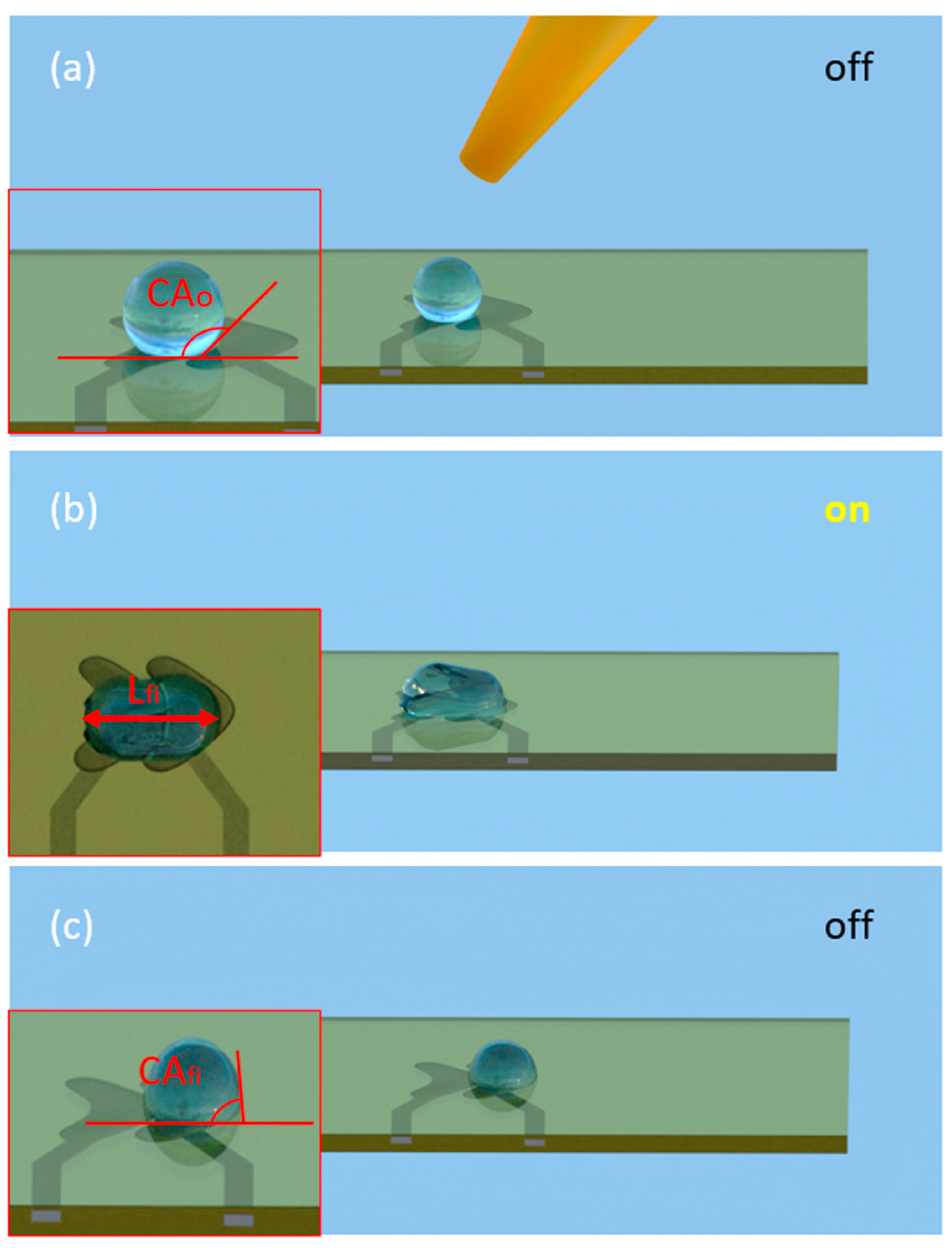
2.1. Sensor Principle

Electrowetting On Dielectric (EWOD) is a microfluidic technology that moves small liquid droplets using electrical fields. We propose to take advantage of this technology to measure the concentration of a dispersant through the change in its surface tension that causes a different droplet deformation between electrodes. Initially, a droplet is placed on the surface of the EWOD device with non-energized electrodes, leading to a specific CA due to surface properties, as depicted in Figure 1a. Upon applying voltage, as shown in Figure 1b, the CA at the droplet–electrode interface undergoes changes, resulting in the asymmetric spreading of the droplet and a reduced CA on the activated side. The electrowetting effect induces the movement of the droplet towards the electrode upon the application of voltage. Although the removal of the voltage restores the initial CA, the droplet retains its new position, as depicted in Figure 1c, signifying displacement. Throughout sensor operation, various parameters of the droplet shape are measured after activating the sensor, including the forward and backward CA, the droplet length and area on the surface.

An EWOD device typically consists of three functional layers on a supporting material. The first layer, known as the electrical layer, features two closely spaced electrodes. The second layer, the dielectric layer, plays a crucial role in preventing electrical contact between the electrodes when it comes into contact with the liquid from the manipulated water droplets on the surface. This dielectric layer is essential for maintaining the integrity of the device and ensuring that electrical signals are properly controlled. The electrical layer, coated with a dielectric layer and a hydrophobic layer, functions as a capacitor. When a voltage is applied across the electrodes, an electromagnetic field is generated, which alters the wetting behavior of the droplet on the device.

The behavior of the EWOD device is described by the Lippmann–Young equation [33] (Equation (1)):

$$cos{\theta }_v-cos{\theta }_0={\displaystyle \frac{C}{2\gamma }}{V}^2$$

where θ₀ is the initial or pre-voltage CA (°) and θ_v is the final or post-voltage CA (°), which are described in terms of the device capacitance (C), applied voltage across the electrodes (V) and surface energy (γ).

In this manner, by observing the initial and final CA (see Figure 1) and using a consistent device with a known voltage (i.e., constant capacitance and voltage), we can determine the liquid’s surface energy [34]. This, coupled with the understanding of the correlation between the concentration of marine dispersant and the surface energy of the solution, enables the use of a sensor like this to determine the concentration of marine dispersant in a liquid sample.

2.2. Capillary Regime Validation

The EWOD sensor relies on the Lippmann equation to relate changes in surface tension to variations in the CA under an applied voltage. This equation assumes that the droplet shape is primarily governed by surface tension rather than gravitational forces. To validate this assumption, the capillary length (l_c) and the Bond number (Bo) were calculated for the tested conditions [34,35].

The capillary length defines the scale above which gravity deforms a droplet and is given by

$$l_c=\sqrt{{\displaystyle \frac{\mathsf{\Upsilon }}{\rho g}}}$$

where ϒ is the surface tension (N/m), ρ the liquid density (kg/m³), and g the gravitational acceleration (9.81 m/s²). It represents the length scale beyond which gravitational forces deform the droplet.

The Bond number, which expresses the ratio of gravitational to capillary forces, was computed using

$$Bo={\displaystyle \frac{\rho g{L}^2}{\mathsf{\Upsilon }}}$$

where L is the characteristic length, taken as the droplet base diameter. These metrics were used to confirm that the system operates within the capillary regime, ensuring the applicability of electrowetting-based surface tension measurements.

2.3. Device Manufacturing Method

A schematic of the device fabrication can be seen in Figure 2. Glass slides were cleaned using a piranha solution, composed of sulfuric acid (H₂SO₄, 96%, Applichem Panreac, Castellar del Vallès, Spain) and hydrogen peroxide (H₂O₂, 30%, Applichem Panreac, Castellar del Vallès, Spain) in a 3:1 (v/v) ratio. They were immersed in the solution for 10 min and subsequently rinsed several times with deionized water. Finally, they were dried at room temperature.

The glass wafer was treated with oxygen plasma for 60 s at 60 W to enhance the adhesion of the subsequent layer before the electrode printing process. Heart-shaped electrodes were directly printed on the plasma-treated glass substrate using silver nanoparticle ink (npAg) (Sicrys ailver nanoparticle ink in diethylene glycol monomethyl ether, PVnanocell, Migdal Ha’Emek, Israel) at a concentration of 20 wt%. The heart-shaped electrode geometry was selected for its higher efficiency in directing droplet movements unidirectionally, enabling the sensor to be optimized for use with the lowest possible voltage [36]. The electrode printing was performed using a Dimatix printer (Model DMP-2831, FUJIFILM Dimatix, Inc., Santa Clara, CA, USA) equipped with Fujifilm Dimatix SAMBA cartridges. For the printing configuration, a single inkjet nozzle was used, operating at a voltage of 25 V. The cartridge temperature was set to 28 °C, while the printing tray temperature was maintained at 40 °C, optimizing the conditions for the ink deposition process. The printing process was executed in two stages. Initially, three layers of npAg ink were applied, focusing on the high-resolution printing of the device’s action electrodes. This step ensures the critical quality of the initial part, as it is essential to achieve a very small gap between electrodes without electrical communication between them. Therefore, high-resolution printing is crucial in this phase before proceeding to print the connection pads linking the electrodes and the power source. Additionally, pre-pattern line printing was configured to guarantee optimal ink charge in the nozzle’s chamber, ensuring effective ink delivery during the printing process. The electrodes were treated a two-stage curing process: initially dried at 50 °C for 15 min and then cured at 130 °C for 60 min, as per the ink manufacturer’s specifications. For this configuration, a printing resolution was achieved that resulted in an electrode gap of 80 µm, as show in Figure 2f, ensuring precise electrode spacing crucial for the device’s functionality.

For the dielectric layer, an epoxy-based negative photoresist (SU-8) (GM1050 from GERSTELTEC SARL, Pully, Switzerland) was used. The wafers were pre-treated with oxygen plasma for 60 s at 60 W to enhance the adhesion of SU-8. This was followed by a spin-coating application at 4200 rpm for 40 s and then pre-curing at 65 °C for 15 min. Subsequently, a 15 s UV exposure was performed, concluding with a post-cure at 130 °C for 15 min.

Before the application of the hydrophobic layer, the device was treated with oxygen plasma for 60 s at 60 W to enhance the layer’s adhesion. A mixture of polydimethylsiloxane (PDMS) (Dow Inc., Midland, CA, USA) was prepared. The coating was applied by spin-coating at 5000 rpm for 1 h to achieve a layer thickness of approximately 5 μm. The device was then left at room temperature for 5 min prior to thermal curing at 80 °C for 2 h.

The gap between electrodes in the electrical layer was measured using the optics of the Dimatix DMP-2831 (FujiFilm Dimatix, Inc., Santa Clara, CA, USA). The thickness and roughness of the electrical, dielectric, and hydrophobic layers were evaluated through white light interferometry (Filmetrics Profilm3D Profilometer), using the Arithmetic mean height (Sa) as the roughness measurement.

The overall fabrication process is based on using known materials from microfluidics or electronics manufacturing such as glass slides, photosensitive resins (SU-8), polymers (PDMS), and nanoparticle silver ink. Its compatibility with standard electronics manufacturing processes offers the opportunity to batch-manufacture the sensor, achieving low manufacturing costs. This fact makes the design suitable for point-of-need applications or single-use deployment in environmental monitoring.

2.4. Preparation of Surfactant Solutions and Tensiometer

The solvent used for all solutions was seawater, specifically from the area of Barcelona at the geographic coordinates 41°15′48.5″ N 1°59′21.3″ E, collected in October 2022. The selection of seawater enhances the extrapolation of the results to real-world scenarios. Seawater samples were stored in 1 L aliquots at 4 °C. The marine dispersant used was MK-Disper (Alaba, Spain), kindly provided by Trafic Medioambiente (Madrid, Spain). Initially, a stock solution of MK-Disper was prepared at a concentration of 1 g/L using seawater as the solvent. The solution was mixed by magnetic stirring for 1 h to ensure the homogenization of the solution.

Thirteen different concentrations of MK-Disper were evaluated to study their impact on surface tension. These concentrations were prepared from a stock solution, with a range from 0.1 g/L to 1.5 g/L. An OCA 15EC contact angle optical tensiometer (Dataphysics, Filderstadt, Germany) was used for the CA measurements. To validate the results with MK-Disper on the device, two additional cationic surfactants were assessed: tetradecyltrimethylammonium bromide (TTAB) (Merck, Darmstadt, Germany) and n-dodecyltrimethylammonium bromide (DTAB) (Merck, Darmstadt, Germany). For TTAB, 14 solutions were prepared with concentrations ranging from 0.08 mM to 2.25 mM. For DTAB, 10 solutions were formulated with concentrations between 0.03 mM and 0.12 mM. These additional tests were conducted to corroborate the validity of the findings with MK-Disper.

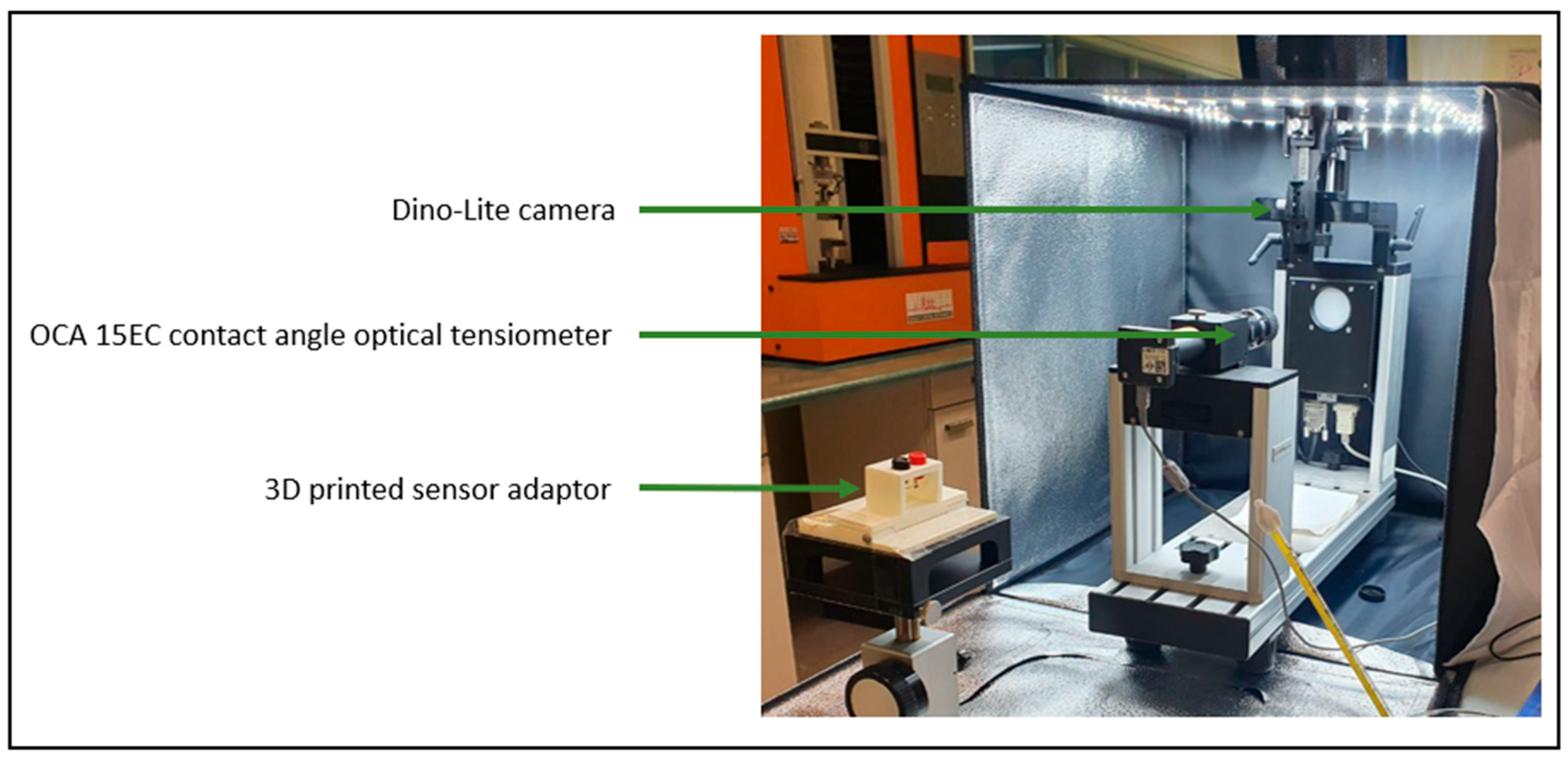
2.5. Experimental Setup

The experimental setup depicted in Figure 3 was used to validate the performance of the sensor. A custom adapter was designed and 3D-printed to facilitate the connection between the EWOD device and the power supply (PASCO scientific SF-9585 model, Roseville, CA, USA). Overhead and sagittal images of the device’s operation were captured both before and after applying the actuation voltage. The sagittal images utilized the optics of an OCA 15EC contact angle optical tensiometer (Dataphysics, Filderstadt, Germany), while overhead images were taken using a Dino-Lite camera (AnMo Electronics Corporation, Hsinchu City, Taiwan). CA, lengths, and areas of the droplets were measured both before and after applying the actuation voltage. In the CA analysis, angles on the advancing side of the droplet (forward CA) and on the opposite side (CA backward) were differentiated. A quantitative analysis of all images was conducted using ImageJ software (version 1.54d).

All measurements and experiments were conducted in a specially conditioned room with strict control of the environmental conditions. The temperature was maintained at a constant 23 °C and the relative humidity (RH) at 50%. These conditions were chosen to ensure the consistency and reproducibility of results, minimizing variability due to external factors.

First, a study was conducted to explore which combination of volume and voltage would yield the most significant differences in the various study variables. These variables included forward and backward CAs, total drop length, and total drop area, both before and after device activation. Subsequently, seawater droplets of different volumes (9 µL, 11 µL, 13 µL, and 15 µL) were placed on the EWOD device and subjected to various voltages (100 V, 150 V, and 200 V) for an analysis of their behavior through overhead and sagittal images. Throughout the measurements, it was ensured that the EWOD device was free of contaminants and in perfect operational condition.

Different concentrations were independently prepared: MK-Disper at 0 g/L, 0.3 g/L, 0.6 g/L, 0.9 g/L, 1.2 g/L, and 2 g/L; TTAB at 0.25 mM, 0.6 mM, 1.1 mM, 1.25 mM, and 1.5 mM; and TDAB at 0.04 mM, 0.06 mM, 0.08 mM, 0.09 mM, and 0.12 mM. Between measurements, the surface of the EWOD device was thoroughly rinsed with deionized water and gently dried with compressed air. This cleaning step was performed to remove any residual salts or surfactant traces from previous droplets, thereby minimizing inter-sample contamination and reducing the potential influence of salt crystallization on CA hysteresis.

2.6. Electrostatic Simulation

To support the interpretation of the experimental results, a numerical simulation was performed using COMSOL Multiphysics^® v6.1, employing the Electrostatics module. A simplified 2D model was constructed to represent the cross-sectional geometry of the EWOD system, including the dielectric layer, surrounding air domain, and a sessile droplet of seawater positioned over a square electrode. A neighboring electrode served as the ground.

The geometry was designed to capture the essential physics while reducing computational complexity. The dielectric layer thickness and applied voltage were matched to the experimental setup (5 µm dielectric and 150 V actuation). Boundary conditions included electrical insulation for all external surfaces and a fixed voltage of 150 V on the actuation electrode. The seawater droplet and air domains were defined with their respective relative permittivity.

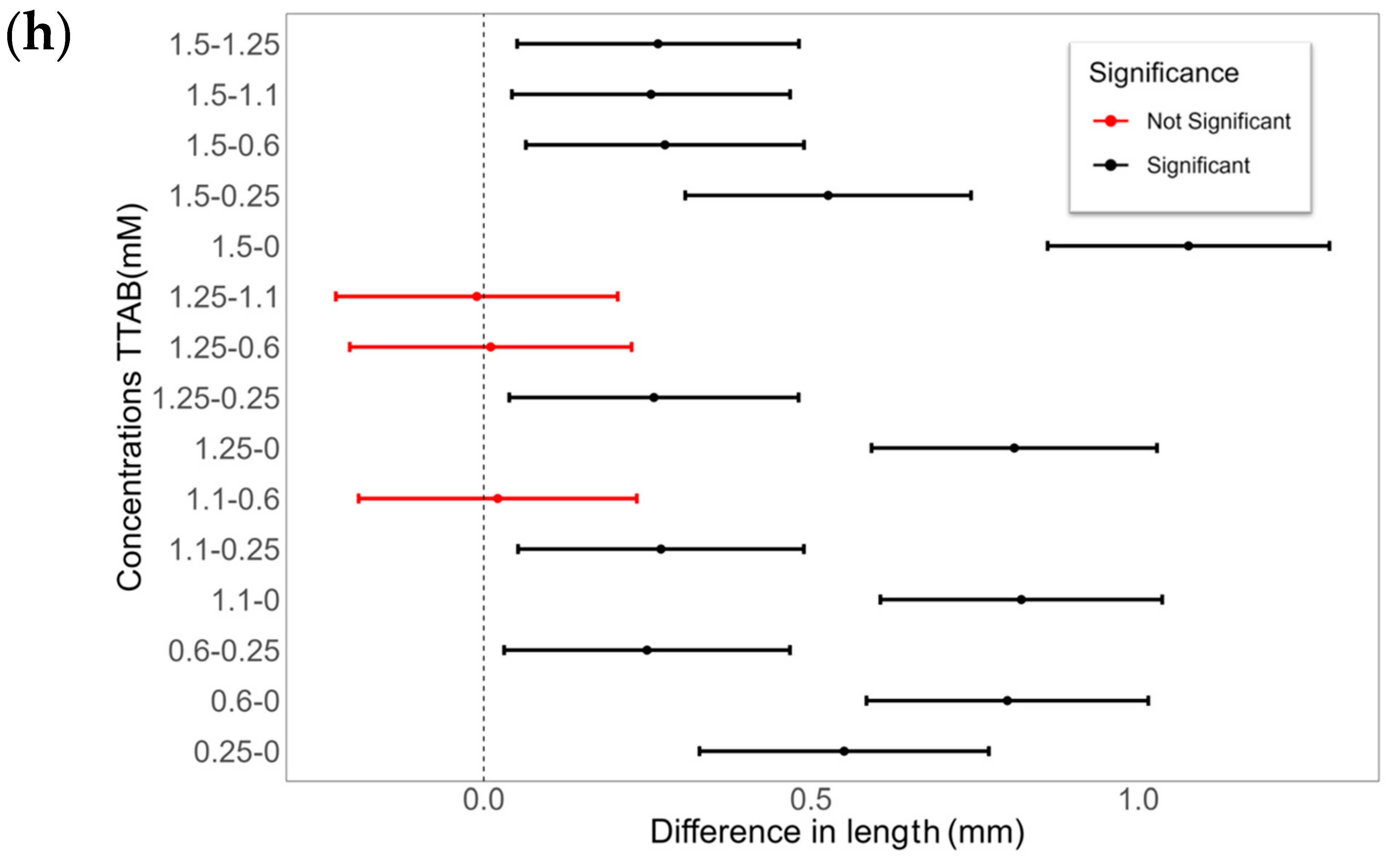
2.7. Statistical Analysis

For analyzing differences among groups, the normality of variable distribution was initially assessed using the Shapiro–Wilk test [37]. Based on the normality results, an analysis of variance (ANOVA) [38] was conducted for data following a normal distribution, or the non-parametric Kruskal–Wallis test [39] was used otherwise. Upon detecting significant differences, post hoc contrasts for multiple comparisons among the five studied groups were performed: Tukey’s HSD test for ANOVA [40] and the Dunn test for Kruskal–Wallis [41]. Both methods incorporate p-value correction to account for multiple comparisons, ensuring statistical reliability in group-wise contrasts [42].

In addition to the aforementioned variance analysis, the size effect for the observed significant differences among the groups was estimated. For this purpose, Cohen’s d measure [43] was employed, quantifying the magnitude of the observed effect in terms of standard deviations. A Cohen’s d of 0.2 is considered a small effect, 0.5 a medium effect, and 0.8 a large effect. Data analysis was performed with R statistical software (version 3.1).

A logarithmic regression was conducted on the observations for both the CA and droplet length on the device to develop a model. Subsequently, the Normalized Mean Absolute Error (NMAE) [44] was calculated to compare the two models. The NMAE adjusts the Mean Absolute Error (MAE) by the range (the difference between the maximum and minimum) of the observed values, providing a relative error metric that is less sensitive to scale differences. To calculate the sensitivity and Limit of Detection (LOD) of the sensor, a logarithmic regression model is employed [45,46]. The sensitivity, corresponding to the slope of the regression line, is derived from the model coefficients. This slope indicates how much the sensor response (the final CA or final length) changes per unit increase in the logarithm of the analyte concentration. The LOD is determined using the standard error of the residuals from the regression and is calculated as three times the standard error divided by the absolute value of the slope. This approach accounts for the variability in the sensor response and provides a threshold below which the signal cannot be reliably distinguished from background noise.

3. Results and Discussion

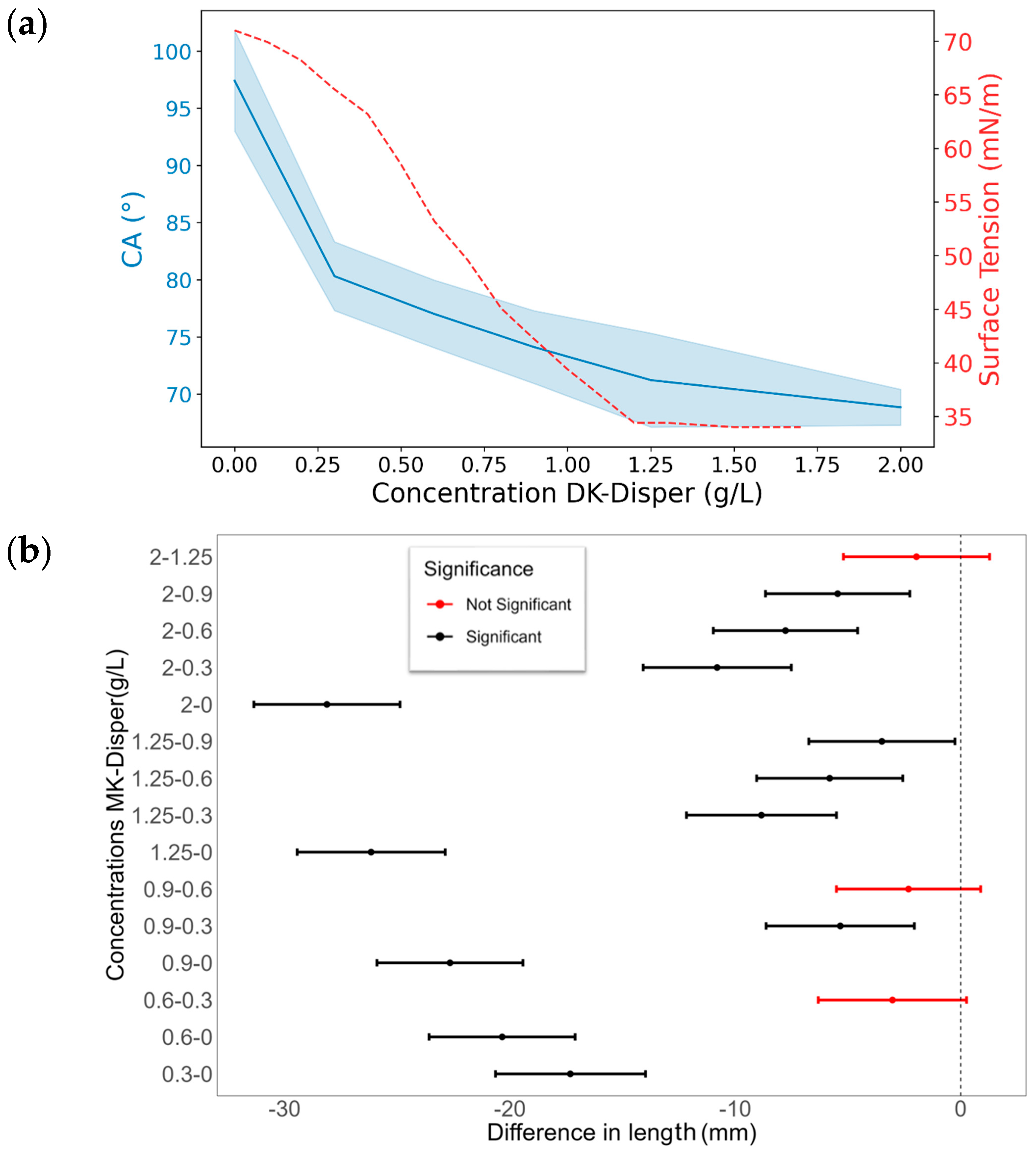
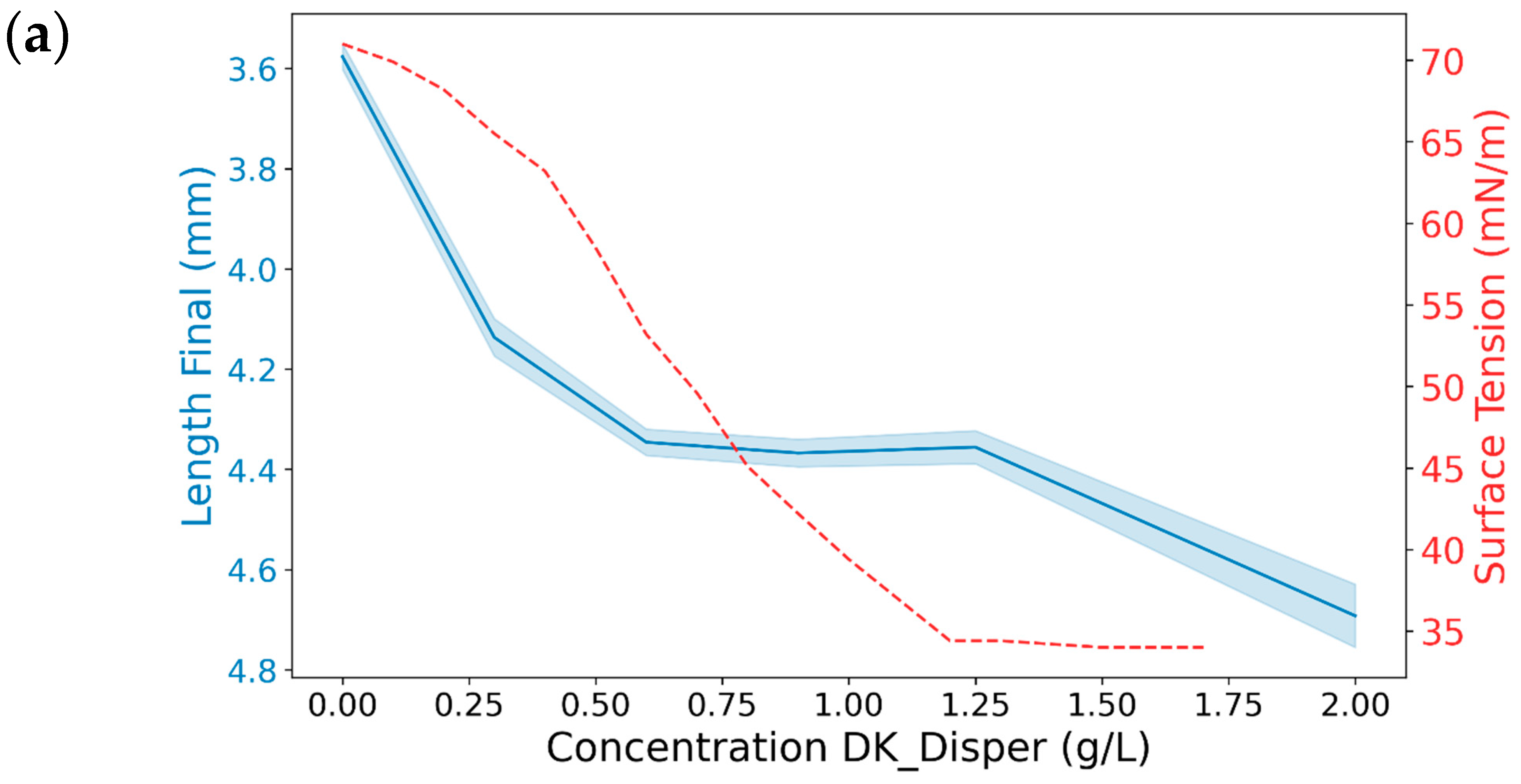
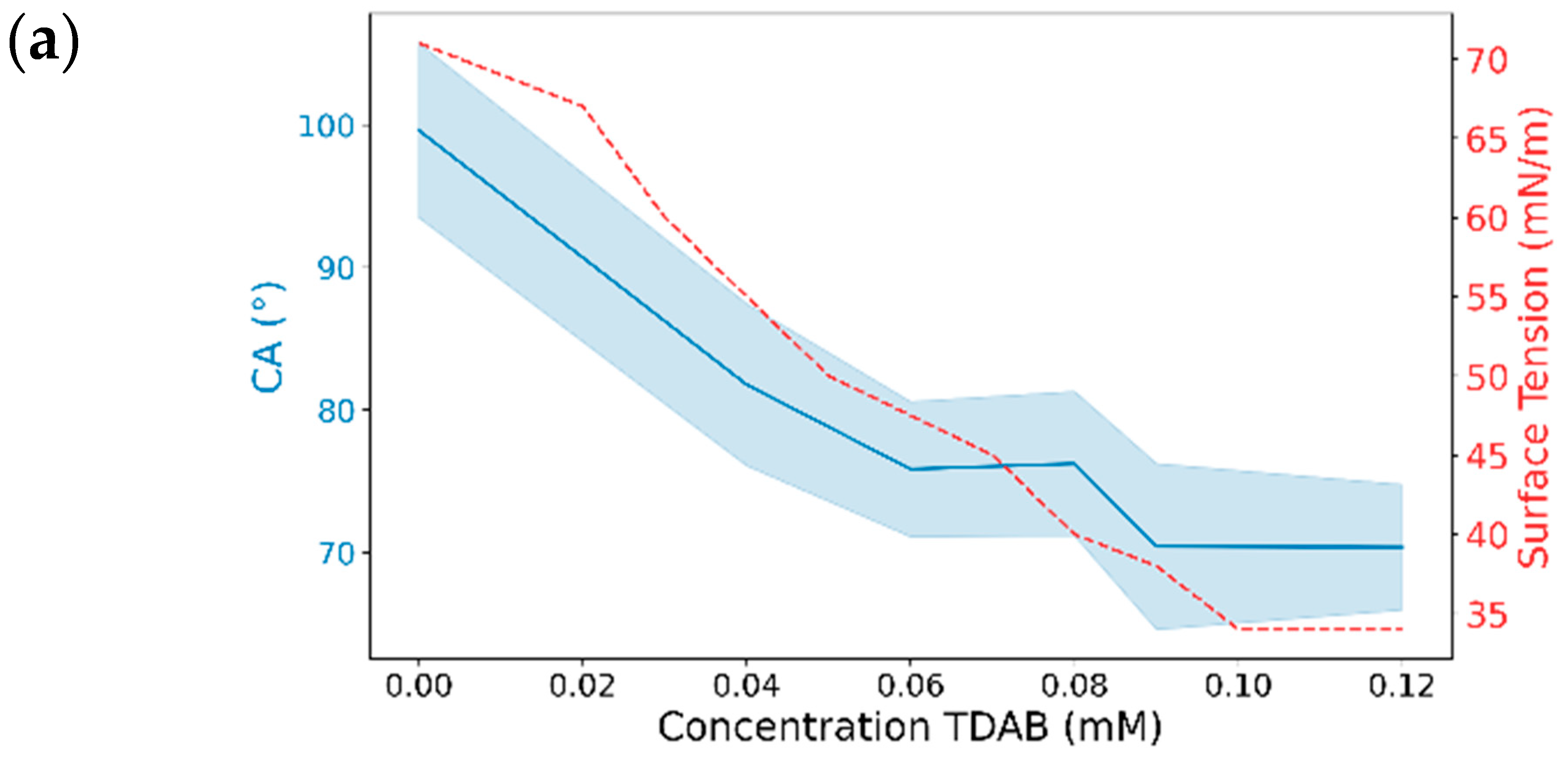
3.1. Impact of Marine Dispersant on Seawater Surface Tension

With the aim of assessing the impact of various concentrations of MK-Disper, TDAB, and TTAB on the static surface tension of seawater, the pendant drop method was employed. The results of these evaluations are presented in Figure 4.

On a logarithmic scale, three linear regimes are identified. The first regime of the MK-Disper isotherm, from 0 to 0.4 g/L, shows a slope defined by SE₁ = −6.74[MK-Disper] + 54.78, with a correlation coefficient R² of 0.97. In this range, surface tension begins to decrease, indicating that dispersant molecules at the air–water interface start to weaken the molecular forces among water molecules, thereby altering the liquid’s surface tension. In the second regime, defined by the isotherm SE₂ = −23.4[MK-Disper] + 40.27 (R² = 0.98), a more pronounced change in surface tension for each additional unit of MK-Disper concentration is observed. This suggests that each increment in the dispersant concentration has a more significant effect in reducing surface tension compared to the first regime. A third regime emerges from 1.2 g/L, characterized by a flattened slope. This behavior indicates the saturation of surfactant molecules at the air–water interface and the onset of the critical micelle concentration (CMC). At higher concentrations, the surface tension stabilizes, signaling the formation of micelles in the liquid.

In Figure 4b,c, the logarithmic concentration function of TDAB and TTAB exhibits a pattern consistent with surfactant behavior. For both surfactants, three regimes are also observed. In the case of TDAB, the first isotherm regime is characterized by SE₁ = −11.01[TDAB] − 32.46 (R² = 0.99). Beyond the concentration threshold of 0.043 mM, the second isotherm regime is evident, described by SE₂ = −32.55[TDAB] − 35.33 (R² = 0.99). The onset of the critical micelle concentration (CMC) occurs at 0.12 mM. For TTAB, the initial regime’s isotherm equation is SE₁ = −4.35[TTAB]x + 59.62 (R² = 0.94). The second isotherm regime appears from a concentration of 0.18 mM, with SE₂ = −13.25[TTAB] + 44.56 (R² = 0.95). The CMC is observed starting from 2 mM.

The observation of these three regimes can be attributed to the presence of an adsorption activation barrier at low concentrations of MK-Disper. This barrier impedes the adsorption of surfactant molecules at minimal dilution [47,48,49,50]. This suggests potential limitations in detecting dispersant concentrations through surface tension at low concentrations. However, at higher concentrations, the impact of this adsorption barrier diminishes, explaining the increased rate of change in surface tension relative to concentration. The strong R² values for MK-Disper, TDAB, and TTAB confirm the linearity of the concentration–surface tension relationship prior to the CMC. These findings corroborate the relationship between MK-Disper concentrations and seawater surface tension, consistent with previous research linking surfactant concentrations to surface tension in aqueous mediums [29,51,52]. Thus, it is feasible to determine the concentration of a dispersant in a marine sample using surface tension, employing a calibration curve with known concentrations of the dispersant. However, reduced accuracy at low concentrations is noted due to the initial adsorption barrier at the air–water interface, potentially impacting direct surface tension measurements at low concentrations.

3.2. Device Characterization

The EWOD device consists of three functional layers on a substrate. The characteristics of each layer are critically important for the fabrication of an effective and durable EWOD device [53]. In the electrical layer, the key parameters include electrode geometry and the gap between them. The thickness of the electrical layer was 1 µm (±0.5) with the printing of three layers of npAg ink. The printing resolution allowed for an 80 µm gap between electrodes without electrical communication between them. The heart-shaped geometry was chosen based on its higher efficiency in unidirectional movement, as reported in the literature [54]. The thickness of the dielectric layer is important to ensure that there will be no dielectric breakdown at a given voltage when handling an ionic liquid like seawater. Reducing the dielectric layer thickness enables droplet manipulation at lower voltages, thus minimizing the risk of an electrical breakdown and prolonging the device’s lifespan [36,54]. The characterization of the dielectric layer of the device through white light interferometry reveals a thickness of 5 µm (±1). The final layer of the device, which is part of its surface, must be highly hydrophobic, with minimal thickness and minimal roughness. This is necessary to minimize the hysteresis exhibited by the droplet on the surface, which can affect its movement. Hysteresis is due to the surface roughness and thickness of the layer [55,56]. Hysteresis could be mitigated by increasing the voltage [57], reducing the thickness of the applied layer [55], or applying an oil layer [58], thus facilitating droplet movement. However, as explained earlier, increasing the voltage significantly reduces the device’s lifespan. Furthermore, introducing oil onto the surface would compromise measurement accuracy in surfactant and dispersant solutions. The implemented PDMS layer exhibits a CA with seawater of 117° (±4), with a layer thickness of 5 µm (±1) and a roughness of Sa = 167 nm.

CA hysteresis and saturation are well-known limitations in EWOD systems. In this study, hysteresis is partially mitigated by maintaining a clean, smooth surface and avoiding oil lubrication, which can alter the wetting response. Although seawater presents a more complex matrix due to its salinity, we observed that the CA on the actuation side decreased consistently with increasing voltage. In particular, for pure seawater without the dispersant, the CA decreased to approximately 85° at 150 V and 80° at 200 V. These results indicate that the system operates below the saturation threshold of CA modulation, preserving effective sensitivity under the studied conditions.

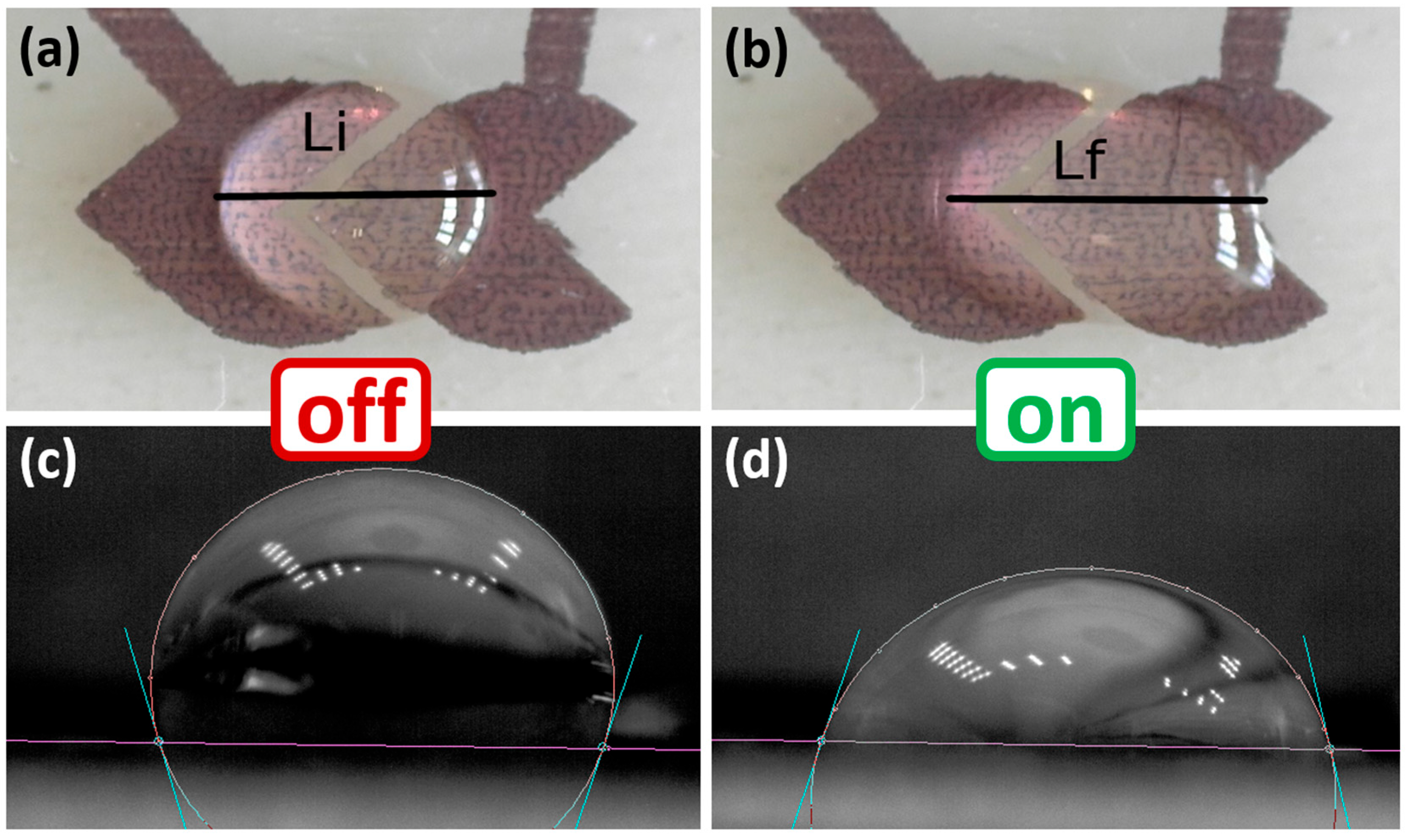
3.3. Volume and Voltage Measurement Methods

In most EWOD devices, the goal is liquid manipulation (mixing, diluting, etc.). However, in this paper, we propose, for the first time, to use EWOD as a sensing technique to determine the liquid’s surface tension and later on correlate this surface tension to the concentration of dispersants. In the proposed configuration, we avoid moving the droplet and we study different variables related to droplet shape, such as the CA or shape, that the droplet adopts depending on the concentration of surfactant when a voltage is applied to it. The studied variables include the CA of the droplet’s front (forward CA) and back (CA backward) after applying voltage. Additionally, the length and area of the droplet were recorded before and after applying voltage to study the differences. The aim is to identify which variables can provide the metrics with the most significant differences among the concentrations. After studying all the variables, it was found that the most significant differences between the different concentrations are the forward CA after voltage and the differences between pre- and post-voltage lengths. Figure 5 displays the analyzed variables: CA and droplet lengths pre and post voltage.

To ensure the applicability of the Lippmann equation, the capillary regime was evaluated by comparing droplet dimensions with the capillary length. For seawater (γ ≈ 72 mN/m), the capillary length is approximately 2.68 mm, while for the lowest surface tension values measured in this study (γ ≈ 33 mN/m), it decreases to around 1.81 mm. The droplets used had a base diameter of approximately 1.5 mm, which remained below the capillary length even at high dispersant concentrations. Furthermore, the Bond number (Bo), which quantifies the relative importance of gravitational forces versus surface tension, was calculated for both cases. For seawater, Bo ≈ 0.31, and for γ = 33 mN/m, Bo ≈ 0.69. Since both values remain below 1, surface tension remains the dominant force shaping the droplet, supporting the validity of using the Lippmann equation under the tested conditions [34].

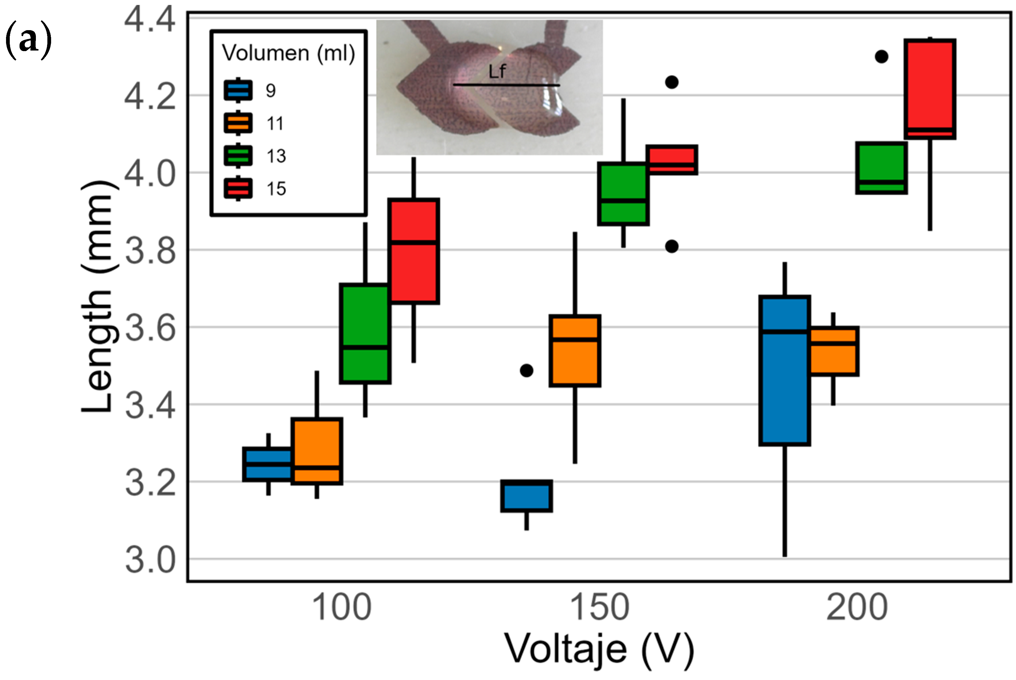
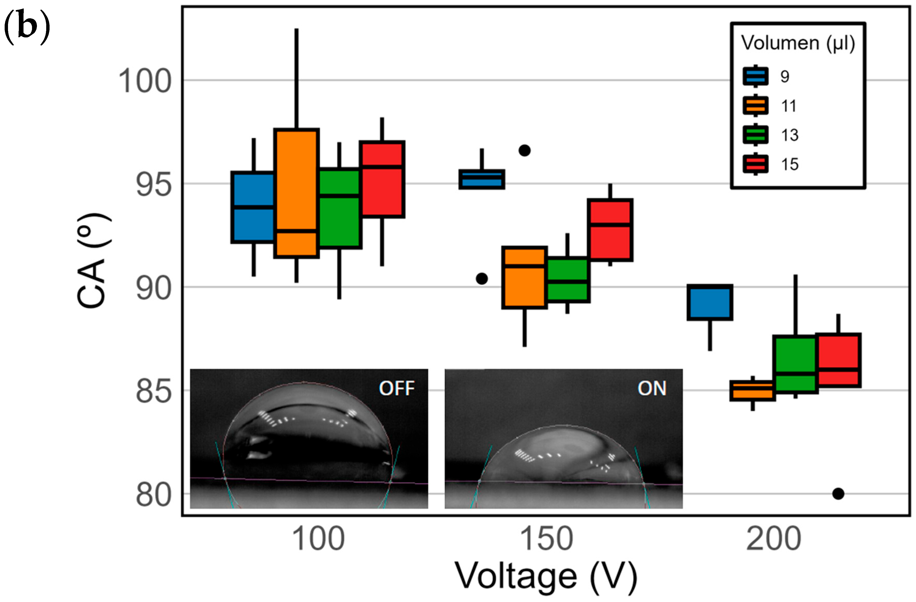
3.4. Parametric Optimization of the Droplet Volume Sensor Actuation Voltage

In order to define the best operation conditions for the sensor, four different droplet volumes of seawater were considered to fully cover the electrode: 9 µL, 11 µL, 13 µL, and 15 µL. To achieve a robust response, three different voltages were tested: 100 V, 150 V, and 200 V. Figure 6a shows the change in length of the droplet once the voltage is applied. Figure 6b shows the change in CA.

This study also allowed us to evaluate the influence of droplet size on the sensor response. Smaller droplets, such as 9 µL, led to greater variability due to a reduced liquid–electrode contact area. In contrast, larger droplets (13–15 µL) provided more stable and sensitive measurements, likely due to enhanced electrowetting efficiency at an increased interface area. Based on these observations, a volume of 13 µL was selected as optimal for the remainder of the experiments.

Figure 6b and Table S1, shows significant differences in the post-activation CA, varying with the droplet volume and applied voltage level. For droplets of 9 µL and 11 µL, there was a CA reduction between 24° and 22°, decreasing from 117° to a range between 93° and 95° at 100 V and 150 V. At 200 V, these volumes experienced a greater CA reduction, reaching 90° and 85° for volumes of 9 µL and 11 µL, respectively. The most notable CA decreases were observed at 200 V for all evaluated volumes and at 150 V for volumes of 11 µL, 13 µL, and 15 µL. With 13 µL and 15 µL, a greater CA reduction between 24° and 32° was recorded at 150 V, resulting in observed CAs of 90° to 92°, respectively. At 200 V, 11 µL, 13 µL, and 15 µL all showed a CA below 86°. These observations suggest that as the droplet volume increases, the influence of voltage on the CA intensifies, which could be due to a larger liquid–substrate interface area exposed to the electric field. In EWOD systems, CA hysteresis can also influence the apparent saturation of the electrowetting effect. While true saturation occurs when further voltage increments no longer reduce the CA due to physical or electrical limits, hysteresis may artificially limit the droplet deformation by anchoring the triple-phase contact line. In our device, the absence of a lubricating layer and the use of a relatively rough PDMS substrate may contribute to this hysteresis. Although CA measurements continued to decrease with increasing voltage—down to 85° at 150 V and 80° at 200 V for pure seawater—suggesting that saturation was not yet reached, it is acknowledged that surface properties could restrict further droplet actuation. High hysteresis may also explain the limited lateral displacement of the droplet observed in some cases, despite measurable changes in CA.

In Figure 6a and Table S2, post-voltage measurements of the droplet length on the device surface are depicted. At 100 V, a gradual increase in droplet length with increasing volume is observed, except for 11 µL, which exhibits a lower total length increase across all voltages. With volumes of 9 µL and 11 µL, significant variability in measurements is noted at 150 V and 200 V. The data for 9 µL and 11 µL may show high variability due to smaller volumes being more dependent on the area of the electrode where the droplet is placed. These differences are not evident with volumes of 13 µL and 15 µL, which seem less dependent on their position on the electrode. In fact, these volumes exhibit a similar length across the three tested voltages, slightly higher at 200 V. These findings indicate that for a greater length and CA change, the ideal volumes are 13 µL and 15 µL, while the voltage showing the most significant differences is 200 V. However, at 200 V, a reduced lifespan of the device is observed compared to its use at 150 V. Taking these findings into account and considering the device’s lifespan and the risk of a dielectric breakdown at higher voltages, it is determined that the 13 µL volume and 150 V are the optimal conditions for discerning differences that may exist among different concentrations of marine dispersant. These conditions offer a balance between obtaining meaningful data and ensuring the device’s safety. Furthermore, the use of 13 µL droplets is consistent with prior studies where droplet volumes in the range of 13–15 µL have been successfully actuated in EWOD devices [59].

In terms of device durability under repeated actuation, based on repeated testing, the device exhibited an average functional lifetime of approximately 20 actuation cycles at 150 V, beyond which increased variability in CA and droplet deformation was observed. Although a physical breakdown (i.e., short-circuit failure) typically occurred after 50 uses at 150 V and between 5 and 15 uses at 200 V, the degradation of the PDMS dielectric surface became evident earlier. This was confirmed by a broader dispersion of data points beyond 20 cycles and visible surface deterioration. Importantly, these measurements were performed using multiple independently fabricated devices under controlled laboratory conditions (temperature and humidity), showing consistent behavior and confirming the reproducibility of the observed degradation trend. These findings suggest that, for reliable operation, the device should be replaced or recalibrated after approximately 20 uses at standard voltage conditions. These findings confirm that such volumes are suitable for stable electrowetting behavior and are within the practical limits for CA modulation. This supports the selection of 13 µL as the optimal working volume in our system, balancing sensor sensitivity, droplet deformation, and device durability.

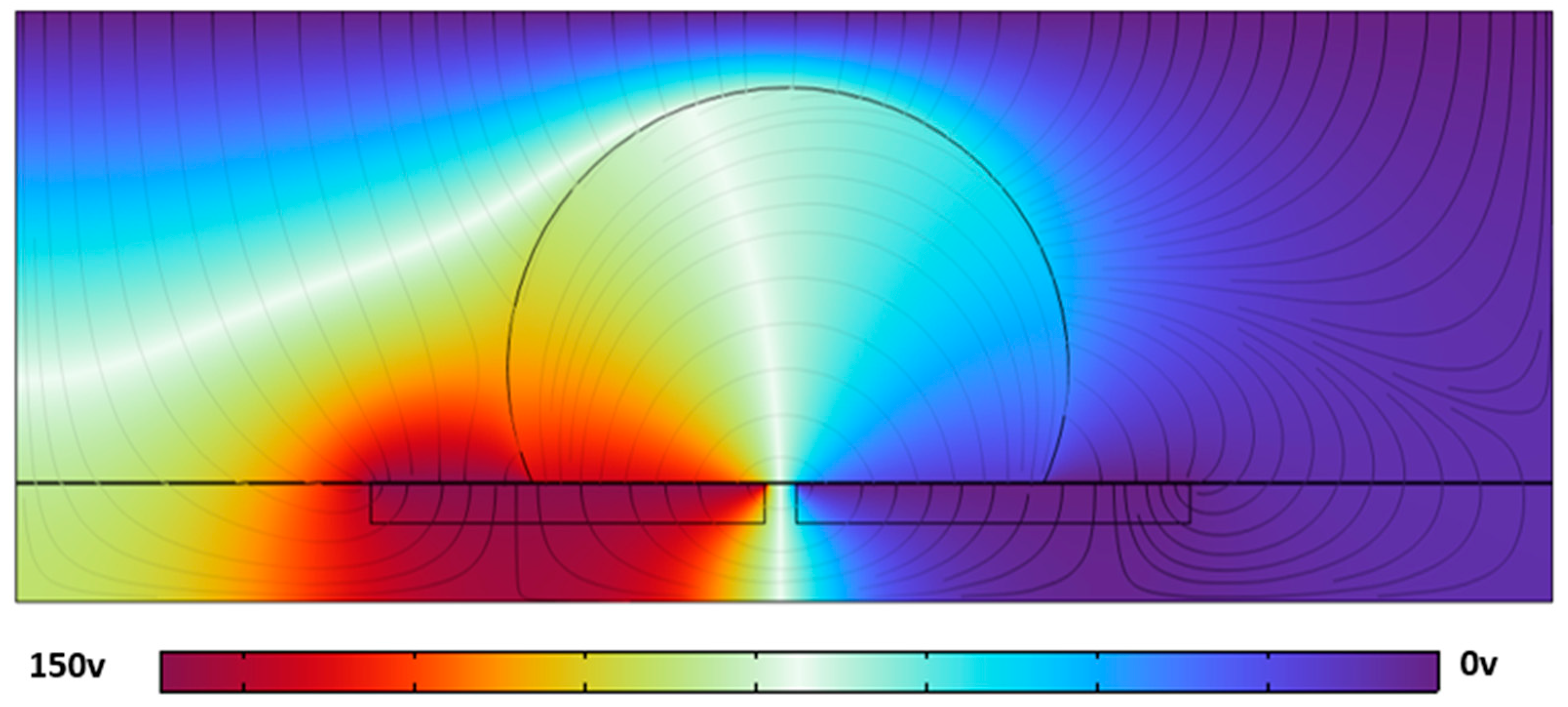
3.5. Numerical Simulation of Electric Field Distribution

To complement the experimental findings and provide a mechanistic insight into the droplet deformation process under electric actuation, a numerical simulation was conducted. The model represents a simplified two-dimensional cross-section of the EWOD device, comprising the fluid (seawater droplet), surrounding air, and dielectric substrate. The droplet is centered above a symmetric square electrode configuration with a ground electrode adjacent to it.

The simulation resolves the electrostatic potential and field lines within the domain, as illustrated in Figure 7. The results clearly show a strong localization of the electric field at the triple-phase contact line between the droplet, substrate, and air. This accumulation of field intensity at the droplet edge supports the observed deformation upon voltage application in the experiments.

Although the electrode geometry and droplet placement are simplified compared to the actual sensor design, this conceptual model captures the essential electromechanical coupling responsible for droplet actuation. It reinforces the hypothesis that deformation is primarily initiated at the droplet boundary due to localized Maxwell stresses.

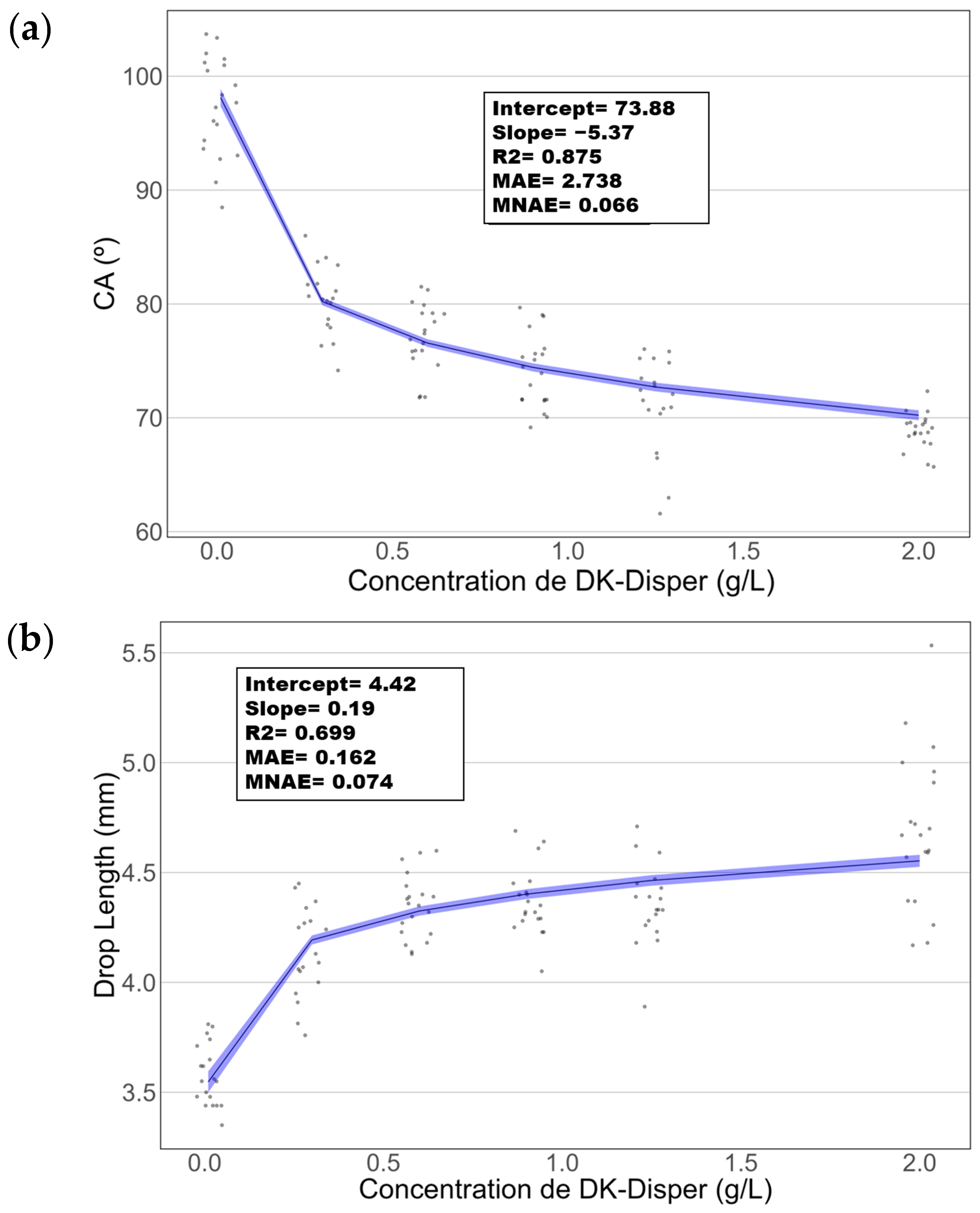
3.6. Sensor Calibration

The CA, lengths, and areas of droplets were analyzed both before and after sensor activation in the presence of different MK-Disper concentrations. This study revealed that the most significant differences with less variability were observed in the forward CA and the length of the droplet post activation compared to the backward CA (Table S3) and the area of the droplet on the device surface (Table S4).

In Figure 8a,b, an analysis of CA after activating an EWOD device with various MK-Disper concentrations is presented. The most marked differences were found in the comparisons at lower concentrations, specifically between 0.3 g/L and 0 g/L and 0.6 g/L and 0 g/L (p-value < 0.001) (Supplementary Table S5). These pronounced differences suggest that the detection method based on the EWOD device could be particularly effective and sensitive at low MK-Disper concentrations, with CA changes of 17° between 0 and 0.3 g/L, compared to smaller changes at higher concentrations, such as 3° between 0.3 and 0.6 g/L. No significant differences were found between concentrations of 0.6 g/L and 0.9 g/L, 0.9 g/L and 1.25 g/L, and between 1.25 g/L and 2 g/L (p-value > 0.05). The lack of differences between 1.25 g/L and 2 g/L aligns with the analysis of their impact on surface tension due to CMC. As concentrations approach CMC, it is common to observe that the surface properties of the solution do not change the CA significantly. This could make the precise detection of marine dispersant concentration challenging. The Cohen’s d values, indicating high effect sizes (Cohen’s d > 0.8), demonstrate the method’s strength in differentiating between the tested concentrations.

Differences in post-activation droplet length across various MK-Disper concentrations are illustrated, as seen in Figure 9a,b. The droplet length following EWOD device activation varies with the concentration of MK-Disper in the solution. Significant differences were detected across most evaluated concentrations. The most notable post-activation droplet length differences were identified between concentrations of 0 g/L and 0.6 g/L, exhibiting a large effect size, with five standard deviations (Cohen’s d = 5.7). This observation aligns with the results from the CA analysis, suggesting that the device might offer a more defined detection of low concentrations compared to common surface tension-based methods, such as the pendant drop or Du Noüy ring methods. No significant differences were observed between concentrations of 0.6 g/L and 1.25 g/L, indicating that, within this concentration range, the sensor is not more effective at measuring MK-Disper concentration than the Du Noüy tensiometer method. This suggests a lower resolution of the sensor within this concentration range compared to the established method. In contrast, concentrations between 1.25 g/L and 2 g/L showed significant differences, suggesting that at these higher concentrations, MK-Disper surfactant properties may more prominently influence droplet deformation. This result is inconsistent with observations from surface tension measurement methods or CA measurement on the device. This could indicate that CMC does not affect post-activation droplet length measurements on the device. A possible explanation is that increased droplet length may enhance the total air–water interface area, allowing a greater absorption of MK-Disper molecules. Additionally, the net charge of certain MK-Disper components, like cationic surfactants, might also affect droplet length, as they are attracted to the charged electrode during activation. This effect is known as the electrophoresis effect, where the charged molecules are attracted to the oppositely charged electrode, pushing the front of the droplet. This effect is greater when the number of charged molecules is greater [60]. This effect could surpass CMC limitations in direct surface tension measurements or CA measurements on the device. However, in maritime conditions, it would not be possible to attain the dispersant’s CMC.

The final CA differences with TDAB and TTAB surfactants are illustrated in Figure 10. Similarly to MK-Disper, as the concentrations of both TDAB and TTAB increase, a generalized decrease in CA is observed. Among TDAB concentrations, significant differences were detected in all cases, except between 0.04 and 0.08 mM (p-value > 0.05), 0.06 and 0.08 mM (p-value = 1), and 0.09 and 0.12 mM (p-value = 1). TTAB exhibited a similar pattern, although at higher concentrations, CA differences were less pronounced. A pattern of significant differences was noted: each concentration was statistically different from all others, except for its nearest adjacent concentration. For example, the 0.25 mM concentration showed significant differences with 0, 1.1, 1.25, and 1.5 mM, but not with 0.6 mM. Similarly, the 0.6 mM concentration was statistically different from 0, 0.25, 1.25, and 1.5 mM, but not from 1.1 mM.

These results are consistent with those obtained with MK-Disper. In the analysis of post-activation droplet lengths with TDAB, fewer significant differences were observed compared to CA. This may be attributed to the lower total concentration of TDAB molecules and their corresponding charge, leading to weaker electrokinetic effects at the droplet’s leading edge and thus less elongation. The largest differences were found between the extreme concentrations (0 mM vs. 0.12 mM: 1.13 mm, 95% CI: 0.84–1.43), while intermediate concentrations (0.04–0.09 mM) showed no significant variation (p > 0.05). In TTAB, a similar pattern emerged, although at high concentrations—near the critical micelle concentration (CMC)—significant length differences were still observed (0.48 mm, 95% CI: 0.18–0.78; p < 0.005). These results support the sensor’s applicability to a range of marine dispersants.

Beyond macroscopic observations, the droplet elongation behavior at high surfactant concentrations may also be influenced by electrohydrodynamic and electrophoretic effects. As the surfactant concentration approaches the CMC, the interface becomes saturated, and further reductions in surface tension diminish, limiting deformation sensitivity. Additionally, the presence of ionic surfactants enables internal electrophoretic transport under the applied electric field. This effect redistributes charges toward the contact line, lowering contact line friction and enhancing wetting dynamics, as shown by Mugele and Baret (2005) [61] and molecular simulations by Johansson and Hess (2020) [62].

Surface charge deposition by moving droplets can further reduce the CA locally, inducing asymmetric spreading. At sufficiently high field intensities, charge redistribution can deform the droplet shape beyond what is predicted by the Lippmann model, especially in ionic systems [60,63]. However, such effects may also introduce nonlinearities and hysteresis, particularly due to charge trapping and dielectric charging [64].

Furthermore, polarity-dependent electro-dewetting has been reported in systems containing cationic surfactants, where low-voltage DC fields (~3 V) can reverse wetting behavior by accumulating surfactant molecules at the solid interface [65,66]. In addition, CA modulation tends to plateau beyond the CMC due to interfacial shielding effects, where further increases in surfactant concentration no longer alter the electric field distribution at the interface [67,68]. These mechanisms have also been exploited in dynamic charge-driven microfluidic systems to induce controlled droplet propulsion [65,66].

In summary, the observed behaviors at high concentrations likely result from the combined influence of interfacial saturation, charge redistribution, and electrokinetic coupling. These phenomena reinforce that under DC actuation, the droplet response is shaped not only by classical interfacial tension changes but also by the nonlinear electrohydrodynamic interplay introduced by surfactants near or above the CMC.

The correlations between surfactant concentrations and the advancing front CA were examined using logarithmic regression models. The choice to employ logarithmic regression models for examining the correlations between surfactant concentrations and the advancing front CA was motivated by the complexity of the relationship between these variables. The experimental data displayed three distinct regimes of behavior as a function of concentration, which could not be adequately captured by a single linear regression model. The logarithmic regression allowed us to summarize the relationship between surfactant concentrations and the CA using a single equation.

As shown in Figure 11a, we can observe the logarithmic model representation of the CA against concentration, while in Figure 11b, the model for droplet length against concentration is illustrated. Both models exhibit statistical significance (p-value < 0.05). Initially, it is noted that CA demonstrates a superior fit, with an R-squared (R²) value of 0.875, compared to the R² of 0.699 for the droplet length. The Mean Absolute Error (MAE) of the CA model is 2.738, contrasting with 0.162 for the droplet length model. Based on these metrics, the CA model possesses a higher R², implying it is better at explaining the data variability compared to the droplet length model. However, comparing the regression coefficients between the hanging drop models, it can be seen that they are somewhat lower, R²_SE = 0.99–0.98 versus R²_CA = 0.875 and R²_L = 0.69. This must be caused by the surface roughness of the device.

Furthermore, although the MAE in the CA model is relatively higher in absolute terms compared to the droplet length model, it is crucial to consider the scale of the dependent variable. An MAE of 2.738 on a scale ranging from 60 to 100 may be relatively small, whereas an MAE of 0.162 on a scale of 3.5 to 5.5 might be deemed more significant. Hence, the Normalized Mean Absolute Error (NMAE) is calculated, revealing values of 6.6% for the CA model and 7.4% for the droplet length model, indicating a good fit between observed and predicted values for both models. Additionally, for the CA model, the sensitivity (slope) is −5.2667, with a Limit of Detection (LOD) of 0.2415 g/L. Conversely, for the droplet length model, the sensitivity is 0.1899, with an LOD of 0.2666 g/L. Considering these findings, the CA model outperforms the droplet length model due to its superior fit, approximately 25.12%. Additionally, the CA model also exhibits a higher LOD compared to the droplet length model. Specifically, the CA model’s LOD is approximately 9.41% better than that of the droplet length model. However, as previously observed, the droplet length model has the advantage of providing better resolution for more concentrated solutions, although such scenarios are highly unlikely in real-world settings.

The sensor exhibited a sensitivity of −5.27 (°CA)/log[g/L] and a detection limit (LOD) of 0.2415 g/L based on the CA analysis of MK Disper. These values confirm the sensor’s ability to detect low concentrations of marine dispersants with high precision. It should be noted that these results are specific to MK Disper and that each dispersant requires an individual calibration curve, as sensor response may vary depending on the formulation and its interfacial effects. The operational principle of the proposed EWOD sensor relies on the application of the Lippmann equation, which relates changes in surface tension to the applied voltage through CA modulation. However, the validity of this relationship assumes that the droplet shape is governed primarily by surface tension rather than gravity. To assess this, we evaluated the capillary regime by calculating the capillary length (lc), which defines the transition scale between capillary and gravitational dominance [34]. For seawater (γ ≈ 72 mN/m), lc ≈ 2.68 mm, while for the lowest surface tension observed in our experiments (γ ≈ 33 mN/m), it decreases to approximately 1.81 mm. Since the droplets used had base diameters between 1.3 and 1.5 mm, they remain below this threshold, suggesting that capillary forces still dominate.

We also calculated the Bond number (Bo), a dimensionless metric quantifying the ratio of gravitational to surface tension forces. For high surface tension, Bo ≈ 0.31, and for γ = 33 mN/m, Bo increases to ≈0.69. Although both values are below 1, indicating a capillary-dominated regime, the rise in Bo at low surface tension implies a growing influence of gravity. This may contribute to the reduced sensor resolution at high dispersant concentrations, where interfacial tension gradients become smaller near the CMC.

These findings support the continued use of the Lippmann equation across the tested range while also delineating its practical limitations as surface tension decreases. These results help delineate the sensor’s theoretical and operational boundaries when applied across a range of surfactant concentrations.

Although the EWOD-based sensor requires a prior calibration curve relating droplet deformation to dispersant concentration, this calibration step inherently accounts for variations in seawater composition. Environmental factors such as salinity, pH, temperature, and dissolved organic matter are known to influence surface tension and, consequently, CA measurements in EWOD systems. These effects have been evaluated in previous works, such as Cai et al. (2016) [30], which showed that natural variability in seawater properties produces only moderate changes in surface tension. In our protocol, a calibration curve is generated using untreated seawater collected on-site and spiked with known concentrations of dispersant. This strategy enables an accurate and robust quantification regardless of the specific water composition or dispersant formulation.

It is acknowledged that under real-life conditions, seawater samples may contain microdroplets of oil in addition to dispersants. These oil residues could potentially affect the measured CA by altering the interfacial properties of the droplet. Although this represents a limitation of the method, it can be mitigated through simple sample preparation strategies. For example, low-speed centrifugation can be applied to remove dispersed oil from the water phase prior to measurement. Alternatively, allowing the sample to rest undisturbed for several minutes enables oil microdroplets to rise and separate naturally due to buoyancy. Either approach can minimize interference and ensure that the measurement reflects the presence of dispersants rather than oil.

In contrast to conventional analytical methods such as HPLC or GC-MS, which offer high sensitivity but require complex sample preparation and laboratory infrastructure, the proposed EWOD sensor provides rapid and in situ quantification with minimal instrumentation. While these laboratory-based techniques are essential for long-term environmental monitoring and toxicological analysis, they are not suitable for real-time decision-making during early spill response operations.

In addition to these direct methods, widely used indirect approaches, such as those assessing dispersant effectiveness through oil dispersion ratios, do not quantify dispersant concentration in water and are typically conducted under controlled laboratory conditions.

Furthermore, widely used indirect methods, such as those assessing dispersant effectiveness through oil dispersion ratios, do not quantify dispersant concentration in water and are typically conducted under controlled laboratory conditions. These techniques are therefore insufficient for evaluating contaminant levels in ecologically sensitive coastal areas. The EWOD-based sensor fills this gap by enabling a point-of-need concentration assessment directly in the field. Although its detection limit (e.g., 0.24 g/L for MK-Disper) is not as low as that of high-end analytical instruments, its portability, speed, and robustness to environmental variability provide a strong advantage in operational marine management contexts.

4. Conclusions

This study has successfully developed and validated a point-of-spill EWOD sensor for quantifying marine dispersants. The sensor offers distinct advantages over traditional surface tension measurement techniques, including improved sensitivity at low concentrations, short acquisition times (within seconds), ease of use in field conditions, and significantly lower cost and complexity. The methodology relies on the effect that dispersants have on the surface tension of a liquid droplet, which leads to different deformation responses when an electric field is applied. An analysis of various variables identified droplet length and the CA as crucial for maximizing sensor sensitivity. The sensor is versatile across dispersant types, with a detection range spanning from concentrations affecting surface tension to the CMC, ranging between 70 mN/m and 40–33 mN/m depending on the dispersant. Since the measurement is based on droplet deformation and surface tension changes, each dispersant requires an individual calibration curve relating surface tension to concentration. This ensures that the sensor can be adapted to different surfactants while maintaining accurate quantification. The measurement of CA change proved efficient and precise for determining dispersant concentration, offering higher resolution at low concentrations compared to conventional surface energy methods. The sensor operates using static image acquisition, capturing the droplet shape immediately before and a few seconds after the application of the voltage. This short delay is sufficient to allow the droplet to reach a stable configuration under the applied electric field. As such, the sensor does not rely on continuous monitoring, but rather on discrete measurements based on steady-state deformation. This approach enables the rapid evaluation of dispersant concentration with minimal latency, typically within seconds of actuation. Its portability and ability to deliver rapid results make it a valuable tool for effective oil spill management, overcoming the limitations of current complex, costly, and land-based laboratory methods that often delay emergency response.

Given the environmental impact of oil spills and the necessity for effective responses, this advancement represents significant progress by providing a practical tool for in situ contamination assessment, enhancing resource management and reducing ecological damage. Although MK-Disper was used in this study due to its common application in the Mediterranean region, the sensor is not limited to this specific formulation. Its design is compatible with any surfactant-based dispersant capable of altering the interfacial properties of seawater. Furthermore, the device is not intended to evaluate dispersant effectiveness, but rather to monitor its presence as a potential contaminant in ecologically sensitive marine zones. This distinction reinforces its role as a decision-support tool in real-time environmental assessment during oil spill response. Lastly, the EWOD device, effective with marine dispersants, could also hold potential for applications involving other contaminants or substances that affect surface tension, enabling rapid in situ analysis.

References

1. Agboola, M.O.; Bekun, F.V.; Joshua, U. Pathway to environmental sustainability: Nexus between economic growth, energy consumption, CO2 emission, oil rent and total natural resources rent in Saudi Arabia. Resour. Policy 2021, 74, 102380. [Google Scholar] [CrossRef]
2. Keramea, P.; Spanoudaki, K.; Zodiatis, G.; Gikas, G.; Sylaios, G. Oil spill modeling: A critical review on current trends, perspectives, and challenges. J. Mar. Sci. Eng. 2021, 9, 181. [Google Scholar] [CrossRef]
3. Chen, J.; Zhang, W.; Wan, Z.; Li, S.; Huang, T.; Fei, Y. Oil spills from global tankers: Status review and future governance. J. Clean. Prod. 2019, 227, 20–32. [Google Scholar] [CrossRef]
4. Asif, Z.; Chen, Z.; An, C.; Dong, J. Environmental impacts and challenges associated with oil spills on shorelines. J. Mar. Sci. Eng. 2022, 10, 762. [Google Scholar] [CrossRef]
5. Tedesco, P.; Balzano, S.; Coppola, D.; Esposito, F.P.; de Pascale, D.; Denaro, R. Bioremediation for the recovery of oil polluted marine environment, opportunities and challenges approaching the Blue Growth. Mar. Pollut. Bull. 2024, 200, 116157. [Google Scholar] [CrossRef]
6. Data & Statistics—ITOPF. 2023. Available online: https://www.itopf.org/knowledge-resources/data-statistics/ (accessed on 16 November 2023).
7. Michael, P.E.; Hixson, K.M.; Haney, J.C.; Satgé, Y.G.; Gleason, J.S.; Jodice, P.G.R. Seabird vulnerability to oil: Exposure potential, sensitivity, and uncertainty in the northern Gulf of Mexico. Front. Mar. Sci. 2022, 9, 880750. [Google Scholar] [CrossRef]
8. Adofo, Y.K.; Nyankson, E.; Agyei-Tuffour, B. Dispersants as an oil spill clean-up technique in the marine environment: A review. Heliyon 2022, 8, e10153. [Google Scholar] [CrossRef]
9. Sharma, K.; Shah, G.; Singh, H.; Bhatt, U.; Singhal, K.; Soni, V. Advancements in natural remediation management techniques for oil spills: Challenges, innovations, and future directions. Environ. Pollut. Manag. 2024, 1, 128–146. [Google Scholar] [CrossRef]
10. Zhu, Z.; Merlin, F.; Yang, M.; Lee, K.; Chen, B.; Liu, B.; Cao, Y.; Song, X.; Ye, X.; Li, Q.K.; et al. Recent advances in chemical and biological degradation of spilled oil: A review of dispersants application in the marine environment. J. Hazard. Mater. 2022, 436, 129260. [Google Scholar] [CrossRef]
11. White, H.K.; Karras, S. The Use of Dispersants in Marine Oil Spill Response. In International Oil Spill Conference; National Academies Press: Washington, DC, USA, 2021; p. 689431. [Google Scholar]
12. Bavadi, M.; Song, X.; Zhu, Z.; Zhang, B. Generation of oil spill dispersants composed of biosurfactants and chemical surfactants: Mechanism exploration through molecular dynamics simulation. J. Environ. Chem. Eng. 2024, 12, 114249. [Google Scholar] [CrossRef]
13. Cui, F.; Geng, X.; Robinson, B.; King, T.; Lee, K.; Boufadel, M.C. Oil droplet dispersion under a deep-water plunging breaker: Experimental measurement and numerical modeling. J. Mar. Sci. Eng. 2020, 8, 230. [Google Scholar] [CrossRef]
14. Prince, R.C. A half century of oil spill dispersant development, deployment and lingering controversy. Int. Biodeterior. Biodegrad. 2023, 176, 105510. [Google Scholar] [CrossRef]
15. Onokare, E.; Odokuma, L.; Sikoki, F.; Nziwu, B.; Iniaghe, P.; Ossai, J. Physicochemical Characteristics and Toxicity Studies of Crude Oil, Dispersant and Crude Oil-Dispersant Test Media to Marine Organisms. J. Niger. Soc. Phys. Sci. 2022, 4, 105–116. [Google Scholar] [CrossRef]
16. Onokare, E.P.; Tesi, G.O.; Odokuma, L.O.; Sikoki, F.D. Effectiveness and toxicity of chemical dispersant in oil spill aquatic environment. Asian J. Water Environ. Pollut. 2022, 19, 41–46. [Google Scholar] [CrossRef]
17. Ozhan, K.; Parsons, M.L.; Bargu, S. How were phytoplankton affected by the Deepwater Horizon oil spill? BioScience 2014, 64, 829–836. [Google Scholar] [CrossRef]
18. Farahani, M.D.; Zheng, Y. The formulation, development and application of oil dispersants. J. Mar. Sci. Eng. 2022, 10, 425. [Google Scholar] [CrossRef]
19. Tiwari, S.K.; Upadhyay, S.; Singh, V.K.; Dasgotra, A.; Umamaheswararao, A.; Sharma, H.; Pandey, J.K. Use of chemical dispersants for management of oil pollution. In Advances in Oil-Water Separation; Elsevier: Amsterdam, The Netherlands, 2022; pp. 263–281. [Google Scholar]
20. French-McCay, D.P.; Robinson, H.; Bock, M.; Crowley, D.; Schuler, P.; Rowe, J.J. Counter-historical study of alternative dispersant use in the Deepwater Horizon oil spill response. Mar. Pollut. Bull. 2022, 180, 113778. [Google Scholar] [CrossRef]
21. Giwa, A.; Chalermthai, B.; Shaikh, B.; Taher, H. Green dispersants for oil spill response: A comprehensive review of recent advances. Mar. Pollut. Bull. 2023, 193, 115118. [Google Scholar] [CrossRef]
22. Quigg, A.; Farrington, J.W.; Gilbert, S.; Murawski, S.A.; John, V.T. A decade of GoMRI dispersant science. Oceanography 2021, 34, 98–111. [Google Scholar] [CrossRef]
23. Fu, H.; Liu, W.; Sun, X.; Zhang, F.; Wei, J.; Li, Y.; Li, Y.; Lu, J.; Bao, M. Assessment of spilled oil dispersion affected by dispersant: Characteristic, stability, and related mechanism. J. Environ. Manag. 2024, 358, 120888. [Google Scholar] [CrossRef]
24. Kujawinski, E.B.; Soule, M.C.K.; Valentine, D.L.; Boysen, A.K.; Longnecker, K.; Redmond, M.C. Fate of Dispersants Associated with the Deepwater Horizon Oil Spill. Environ. Sci. Technol. 2011, 45, 1298–1306. [Google Scholar] [CrossRef]
25. Mathew, J.; Schroeder, D.L.; Zintek, L.B.; Schupp, C.R.; Kosempa, M.G.; Zachary, A.M.; Schupp, G.C.; Wesolowski, D.J. Dioctyl sulfosuccinate analysis in near-shore Gulf of Mexico water by direct-injection liquid chromatography–tandem mass spectrometry. J. Chromatogr. A 2012, 1231, 46–51. [Google Scholar] [CrossRef]
26. Ramirez, C.E.; Batchu, S.R.; Gardinali, P.R. High sensitivity liquid chromatography tandem mass spectrometric methods for the analysis of dioctyl sulfosuccinate in different stages of an oil spill response monitoring effort. Anal. Bioanal. Chem. 2013, 405, 4167–4175. [Google Scholar] [CrossRef] [PubMed]
27. Bugden, J.; Yeung, C.; Kepkay, P.; Lee, K. Application of ultraviolet fluorometry and excitation–emission matrix spectroscopy (EEMS) to fingerprint oil and chemically dispersed oil in seawater. Mar. Pollut. Bull. 2008, 56, 677–685. [Google Scholar] [CrossRef]
28. Abou-Khalil, C.; Ji, W.; Prince, R.C.; Coelho, G.M.; Nedwed, T.J.; Lee, K.; Boufadel, M.C. Field fluorometers for assessing oil dispersion at sea. Mar. Pollut. Bull. 2023, 192, 115143. [Google Scholar] [CrossRef]
29. Fu, J.; Cai, Z.; Gong, Y.; O’reilly, S.; Hao, X.; Zhao, D. A new technique for determining critical micelle concentrations of surfactants and oil dispersants via UV absorbance of pyrene. Colloids Surf. A Physicochem. Eng. Asp. 2015, 484, 1–8. [Google Scholar] [CrossRef]
30. Cai, Z.; Gong, Y.; Liu, W.; Fu, J.; O’Reilly, S.; Hao, X.; Zhao, D. A surface tension based method for measuring oil dispersant concentration in seawater. Mar. Pollut. Bull. 2016, 109, 49–54. [Google Scholar] [CrossRef]
31. Kalli, M.; Chagot, L.; Angeli, P. Comparison of surfactant mass transfer with drop formation times from dynamic interfacial tension measurements in microchannels. J. Colloid Interface Sci. 2022, 605, 204–213. [Google Scholar] [CrossRef]
32. Kleinheins, J.; Shardt, N.; El Haber, M.; Ferronato, C.; Nozière, B.; Peter, T.; Marcolli, C. Surface tension models for binary aqueous solutions: A review and intercomparison. Phys. Chem. Chem. Phys. 2023, 25, 11055–11074. [Google Scholar] [CrossRef] [PubMed]
33. Wang, W.; Xu, S.; Wang, Y.; Chen, X. Contact angle hysteresis due to electric inhomogeneity of topographical patterning of dielectric layer in electrowetting. Colloids Surf. A Physicochem. Eng. Asp. 2024, 699, 134728. [Google Scholar] [CrossRef]
34. Xu, X.; Wang, F.; Qin, Z.; Wen, B. Electrowetting lattice Boltzmann method for micro- and nano-droplet manipulations. Phys. Rev. E 2023, 107, 045305. [Google Scholar] [CrossRef] [PubMed]
35. Feng, X.; Kim, Y.; Park, K.-S. Re-equilibrium of sessile droplets on vertically vibrating substrates. Microsyst. Technol. 2023, 29, 1129–1136. [Google Scholar] [CrossRef]
36. Wang, W.; Rui, X.; Sheng, W.; Wang, Q.; Wang, Q.; Zhang, K.; Riaud, A.; Zhou, J. An asymmetric electrode for directional droplet motion on digital microfluidic platforms. Sens. Actuators B Chem. 2020, 324, 128763. [Google Scholar] [CrossRef]
37. Razali, N.M.; Wah, Y.B. Power comparisons of shapiro-wilk, kolmogorov-smirnov, lilliefors and anderson-darling tests. J. Stat. Model Anal. 2011, 2, 21–33. [Google Scholar]
38. Shapiro, S.S.; Wilk, M.B. An analysis of variance test for normality (complete samples). Biometrika 1965, 52, 591–611. [Google Scholar] [CrossRef]
39. Ostertagová, E.; Ostertag, O.; Kováč, J. Methodology and application of the Kruskal-Wallis Test. Appl. Mech. Mater. 2014, 611, 115–120. [Google Scholar] [CrossRef]
40. Abdi, H.; Williams, L.J. Newman-Keuls test and Tukey test. Encycl. Res. Des. 2010, 2, 897–902. [Google Scholar]
41. Dinno, A. Nonparametric pairwise multiple comparisons in independent groups using Dunn’s test. Stata J. Promot. Commun. Stat. Stata 2015, 15, 292–300. [Google Scholar] [CrossRef]
42. Schlegel, A. Post-Hoc Analysis: Tukey HSD in R. RPubs, 2017. Available online: https://rpubs.com/aaronsc32/post-hoc-analysis-tukey (accessed on 5 May 2025).
43. Rice, M.E.; Harris, G.T. Comparing effect sizes in follow-up studies: ROC Area, Cohen’s d, and r. Law Hum. Behav. 2005, 29, 615–620. [Google Scholar] [CrossRef]
44. Moulahoum, H.; Ghorbanizamani, F. The LOD paradox: When lower isn’t always better in biosensor research and development. Biosens. Bioelectron. 2024, 264, 116670. [Google Scholar] [CrossRef]
45. Gegenschatz, S.A.; Chiappini, F.A.; Teglia, C.M.; de la Peña, A.M.; Goicoechea, H.C. Binding the gap between experiments, statistics, and method comparison: A tutorial for computing limits of detection and quantification in univariate calibration for complex samples. Anal. Chim. Acta. 2022, 1209, 339342. [Google Scholar] [CrossRef] [PubMed]
46. Donati, G. The Case of the Limit of Detection. Braz. J. Anal. Chem. 2022, 9, 8–9. [Google Scholar] [CrossRef]
47. Svitova, T.; Wetherbee, M.; Radke, C. Dynamics of surfactant sorption at the air/water interface: Continuous-flow tensiometry. J. Colloid Interface Sci. 2003, 261, 170–179. [Google Scholar] [CrossRef]
48. Reichert, M.D.; Walker, L.M. Interfacial tension dynamics, interfacial mechanics, and response to rapid dilution of bulk surfactant of a model oil–water-dispersant system. Langmuir 2013, 29, 1857–1867. [Google Scholar] [CrossRef]
49. Peng, M.; Duignan, T.T.; Nguyen, C.V.; Nguyen, A.V. From surface tension to molecular distribution: Modeling surfactant adsorption at the air–water interface. Langmuir 2021, 37, 2237–2255. [Google Scholar] [CrossRef]
50. Mabrouk, M.M.; Hamed, N.A.; Mansour, F.R. Spectroscopic methods for determination of critical micelle concentrations of surfac-tants; a comprehensive review. Appl. Spectrosc. Rev. 2023, 58, 206–234. [Google Scholar] [CrossRef]
51. Myers, D. Surfaces, Interfaces, and Colloids; Wiley: New York, NY, USA, 1999; Volume 415. [Google Scholar]
52. Menger, F.M.; Shi, L.; Rizvi, S.A.A. Re-evaluating the Gibbs analysis of surface tension at the air/water interface. J. Am. Chem. Soc. 2009, 131, 10380–10381. [Google Scholar] [CrossRef]
53. Caro-Pérez, O.; Casals-Terré, J.; Roncero, M.B. Materials and Manufacturing Methods for EWOD Devices: Current Status and Sustainability Challenges. Macromol. Mater. Eng. 2023, 308, 2200193. [Google Scholar] [CrossRef]
54. Son, Y.; Kim, W.; Lee, D.; Chung, S.K. Study on repetitive damage-recovery cycle of hydrophobic coating for electrowetting-on-dielectric (EWOD) applications. Micro Nano Syst. Lett. 2024, 12, 4. [Google Scholar] [CrossRef]
55. Chakrabarty, K.; Zeng, J. Design Automation Methods and Tools for Microfluidics-Based Biochips; Springer: Berlin/Heidelberg, Germany, 2006. [Google Scholar]
56. Sohail, S.; Das, S.; Biswas, K. Effect of Interface Layer Capacitance on Polydimethylsiloxane in Electrowetting-on-Dielectric Actuation. J. Exp. Phys. 2015, 2015, 426435. [Google Scholar] [CrossRef]
57. Cho, S.K.; Moon, H.; Kim, C.-J. Creating, transporting, cutting, and merging liquid droplets by electrowetting-based actuation for digital microfluidic circuits. J. Microelectromech. Syst. 2003, 12, 70–80. [Google Scholar] [CrossRef]
58. Brassard, D.; Malic, L.; Normandin, F.; Tabrizian, M.; Veres, T. Water-oil core-shell droplets for electrowetting-based digital microfluidic devices. Lab Chip 2008, 8, 1342–1349. [Google Scholar] [CrossRef] [PubMed]
59. Sun, D.; Böhringer, K.F. EWOD-aided droplet transport on texture ratchets. Appl. Phys. Lett. 2020, 116, 093702. [Google Scholar] [CrossRef]
60. Bhattacharjee, S.; Khan, S. Molecular insights into the electrowetting behavior of aqueous ionic liquids. Phys. Chem. Chem. Phys. 2022, 24, 1803–1813. [Google Scholar] [CrossRef]
61. Mugele, F.; Baret, J.C. Electrowetting: From basics to applications. J. Phys. Condens. Matter. 2005, 17, R705. [Google Scholar] [CrossRef]
62. Johansson, P.; Hess, B. Electrowetting diminishes contact line friction in molecular wetting. Phys. Rev. Fluids 2020, 5, 064203. [Google Scholar] [CrossRef]
63. Li, X.; Ratschow, A.D.; Hardt, S.; Butt, H.-J. Surface charge deposition by moving drops reduces contact angles. Phys. Rev. Lett. 2023, 131, 228201. [Google Scholar] [CrossRef]
64. Wang, W.; Zhou, J.; Xie, Y. Frequency-dependent contact angle hysteresis in electrowetting. Phys. Fluids 2022, 34, 121702. [Google Scholar] [CrossRef]
65. Zhou, L.; Zhang, Z.; Tang, Y.; Men, C.; Luo, Y.; Wang, H.-T.; Liu, Y. Polarity-dependent electro-wetting/-dewetting for efficient droplet manipulation. Phys. Fluids 2024, 36, 031705. [Google Scholar] [CrossRef]
66. Li, J.; Ha, N.S.; Liu, T.L.; van Dam, R.M.; Kim, C.J. Ionic-surfactant-mediated electro-dewetting for digital microfluidics. Nature 2019, 572, 507–510. [Google Scholar] [CrossRef]
67. Raccurt, O.; Berthier, J.; Clementz, P.; Borella, M.; Plissonnier, M. On the influence of surfactants in electrowetting systems. J. Micromechanics Microengineering 2007, 17, 2217–2223. [Google Scholar] [CrossRef]
68. Roques-Carmes, T.; Gigante, A.; Commenge, J.-M.; Corbel, S. Use of surfactants to reduce the driving voltage of switchable optical elements based on electrowetting. Langmuir 2009, 25, 12771–12779. [Google Scholar] [CrossRef]
Figure 1. Operation scheme of EWOD sensor. (a) A water droplet is placed on the EWOD surface with no voltage applied (“off” state). The initial contact angle (CA0) is defined by the intrinsic surface tension and substrate properties. (b) When a voltage is applied (“on” state), the electrowetting effect reduces the contact angle on the activated electrode, producing an asymmetric droplet shape and droplet spreading. The resulting deformation is quantified by measuring the droplet length (Lfi). (c) After deactivating the voltage (“off” state), the droplet maintains its displaced position on the substrate. The contact angle at the final position (CAfi) is measured to further assess interfacial changes related to dispersant concentration.
Jsan 14 00054 g001
Figure 2. The fabrication steps and structural overview of the EWOD device. (a) The deposition of nanoparticle silver ink (npAg) electrodes, followed by drying at 50 °C and curing at 130 °C. (b) The spin-coating of the SU-8 dielectric layer, including prebake (65 °C, 15 min), UV exposure (15 s), and hardbake (130 °C, 15 min). (c) The spin-coating of the PDMS layer, cured at 80 °C for 15 min. (d) A cross-sectional schematic of the final multilayer structure, showing the sequential stacking of the conductive, dielectric, and hydrophobic layers. (e) An optical image of the fabricated heart-shaped electrodes. (f) A microscopic image of the inter-electrode gap, measuring 80 µm.
Jsan 14 00054 g002
Figure 3. The experimental setup for activating the sensor and conducting experimental measurements.
Jsan 14 00054 g003
Figure 4. An analysis of surface tension in relation to the logarithmic concentration of (a) MK-Disper, (b) TDAB, and (c) TTAB. The red line represents the first observed isotherm regime, the blue line denotes the second isotherm regime, and the black line indicates the critical micelle concentration (CMC).
Jsan 14 00054 g004aJsan 14 00054 g004b
Figure 5. (a) The droplet length on the sensor before activation, (b) the droplet length after applying voltage to the device, (c) the CA of the droplet on the device before activation, and (d) the CA after activation.
Jsan 14 00054 g005
Figure 6. A comparison of the final length and forward CA differences between pre- and post-voltage values by volume and voltage in the EWOD device. N = 25 for each volume–voltage pair. (a) The final length post voltage based on the voltage for various volumes. The color shades in the boxes indicate specific volumes, as detailed in the legend. Outliers are represented as individual data points outside the boxes. (b) Variation in the CA post voltage in relation to the applied voltage for different droplet volumes.
Jsan 14 00054 g006aJsan 14 00054 g006b
Figure 7. The simulated electric potential distribution (color map, in volts) and field lines around a droplet centered on a square electrode in a simplified 2D EWOD system. The maximum field concentration occurs at the triple-phase contact line. The color scale represents the electrostatic potential from 0 to 150 V.
Jsan 14 00054 g007
Figure 8. The effects of different MK-Disper concentrations on droplet properties in an EWOD device operated at 150 V with a 13-Microliter droplet volume. (a) In blue, the correlation illustrates the mean final CA of the droplet on the sensor after activation, corresponding to each concentration level of the dispersant DK-Disper. The shaded area represents the standard deviation (SD) of the measurements. The correlation between the surface energy measured by concentration is depicted by a red dashed line. (b) A comparative analysis of the differences in the advancing front CA across various concentrations, with red dots indicating non-significant differences and black dots representing significant differences (p-value < 0.05). N = 20 for each concentration.
Jsan 14 00054 g008
Figure 9. The effects of different MK-Disper concentrations on droplet properties in an EWOD device operated at 150 V with a 13-Microliter droplet volume. (a) In blue, the correlation illustrates the mean final length (mm) of the droplet on the sensor after activation, corresponding to each concentration level of the dispersant DK-Disper. The shaded area represents the SD of the measurements. The correlation between the surface energy measured by concentration is depicted by a red dashed line. (b) A comparative analysis of the differences in post-activation droplet length across different concentrations, with red and black dots denoting the significance of the observed differences (p-value < 0.05). N = 20 for each concentration.
Jsan 14 00054 g009aJsan 14 00054 g009b
Figure 10. The effect of TDAB and TTAB concentration on the CA and droplet length. (a,c,e,g) CA (°) and surface tension (mN/m) as a function of surfactant concentration for TDAB (a,c) and TTAB (e,g). Blue lines represent the CA or droplet length (left axis) with shaded confidence intervals, while red dashed lines represent surface tension (right axis). (b,d,f,h) Pairwise statistical comparisons of droplet length at different surfactant concentrations for TDAB (b,d) and TTAB (f,h). Each point represents the mean difference between concentration pairs with 95% confidence intervals. Red and black lines indicate non-significant and significant differences, respectively.
Jsan 14 00054 g010aJsan 14 00054 g010bJsan 14 00054 g010cJsan 14 00054 g010dJsan 14 00054 g010e
Figure 11. A graphical representation of logarithmic regressions to evaluate the effect of (a) the CA and (b) length drop of DK-Disper concentrations on the advancing front CA.
Jsan 14 00054 g011
Disclaimer/Publisher’s Note: The statements, opinions and data contained in all publications are solely those of the individual author(s) and contributor(s) and not of MDPI and/or the editor(s). MDPI and/or the editor(s) disclaim responsibility for any injury to people or property resulting from any ideas, methods, instructions or products referred to in the content.