Author Contributions
Conceptualization, A.H.E.F., S.S. and A.M.; methodology, A.H.E.F., S.S. and A.M.; software, A.H.E.F. and S.S.; validation, A.H.E.F., S.S. and A.M.; formal analysis, A.H.E.F., S.S. and A.M.; investigation, A.H.E.F., S.S., N.A.I. and A.M.; resources, A.H.E.F. and S.S.; data curation, A.H.E.F., S.S., N.A.I. and A.M.; writing—original draft preparation, A.H.E.F. and S.S.; writing—review and editing, A.H.E.F., S.S., N.A.I., A.M. and H.E.G.; visualization, A.H.E.F., S.S., N.A.I. and A.M.; supervision, A.M.; project administration, A.M.; funding acquisition, A.M. All authors have read and agreed to the published version of the manuscript.
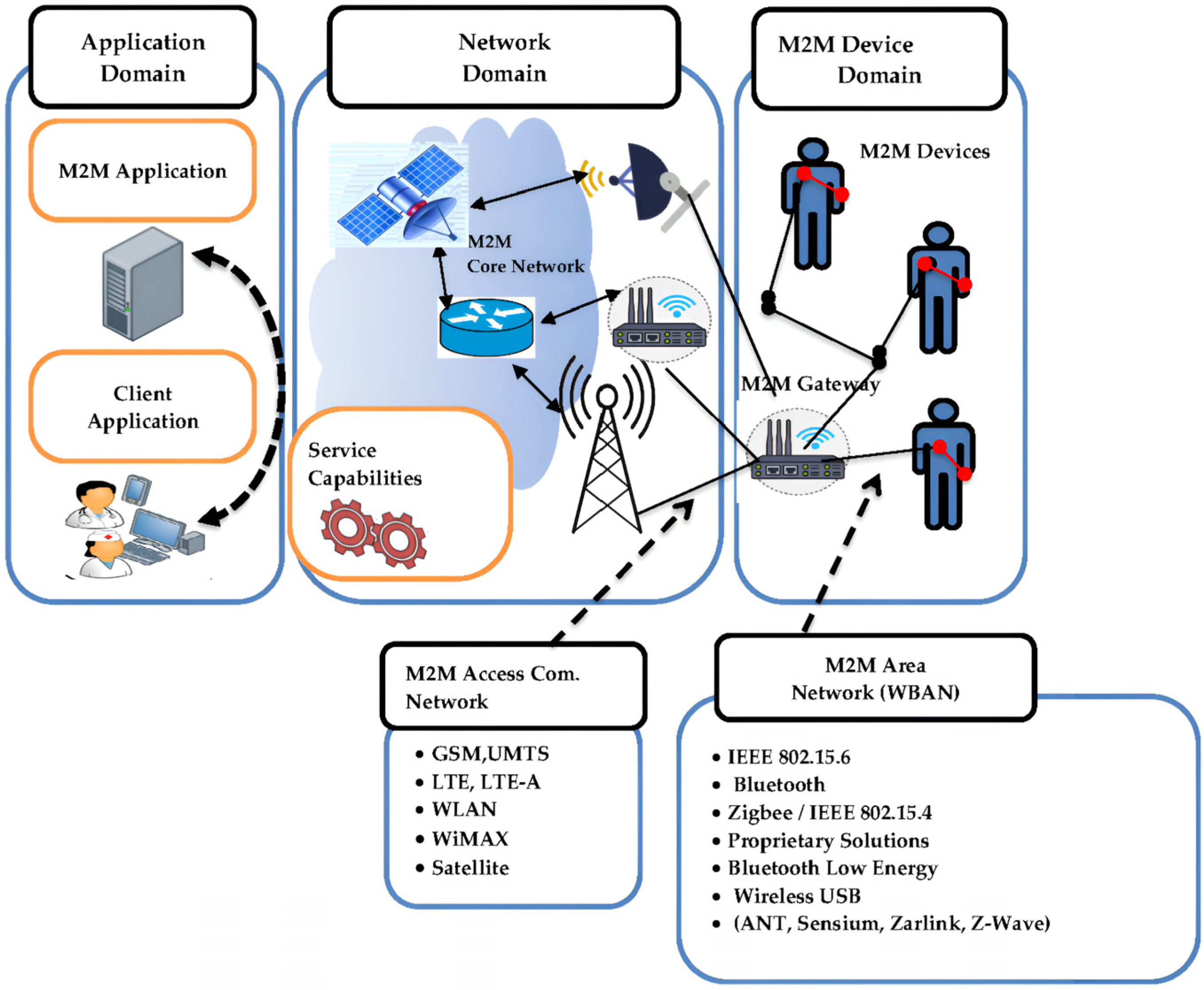
Figure 1.
SOS traffic in M2M domains.
Figure 1.
SOS traffic in M2M domains.
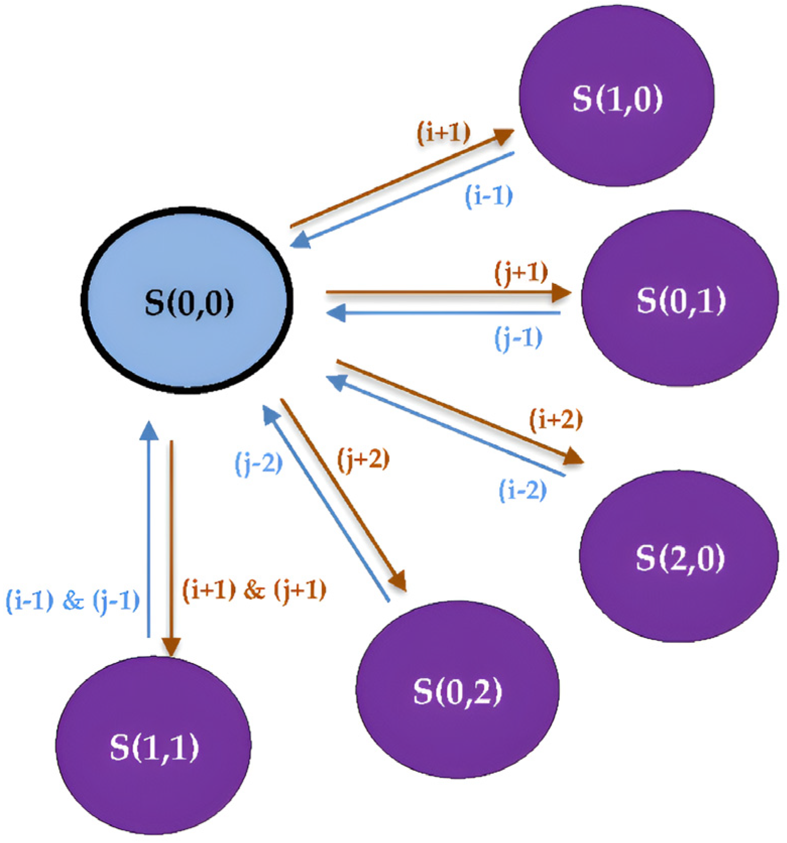
Figure 2.
The CTMC model for C = 3, where “C” is the number of resource blocks available in the network, “S (i,j)” are the states in each phase, “i” represents the number of ongoing M2M services, and “j” represents the number of ongoing H2H services.
Figure 2.
The CTMC model for C = 3, where “C” is the number of resource blocks available in the network, “S (i,j)” are the states in each phase, “i” represents the number of ongoing M2M services, and “j” represents the number of ongoing H2H services.
Figure 3.
The transitioning example from S (0,0) in the “Empty Phase” to the different states in the “Occupied Phase”; “S (i,j)” represents the different states, where “i” is the number of ongoing M2M services and “j” is the number of ongoing H2H services.
Figure 3.
The transitioning example from S (0,0) in the “Empty Phase” to the different states in the “Occupied Phase”; “S (i,j)” represents the different states, where “i” is the number of ongoing M2M services and “j” is the number of ongoing H2H services.
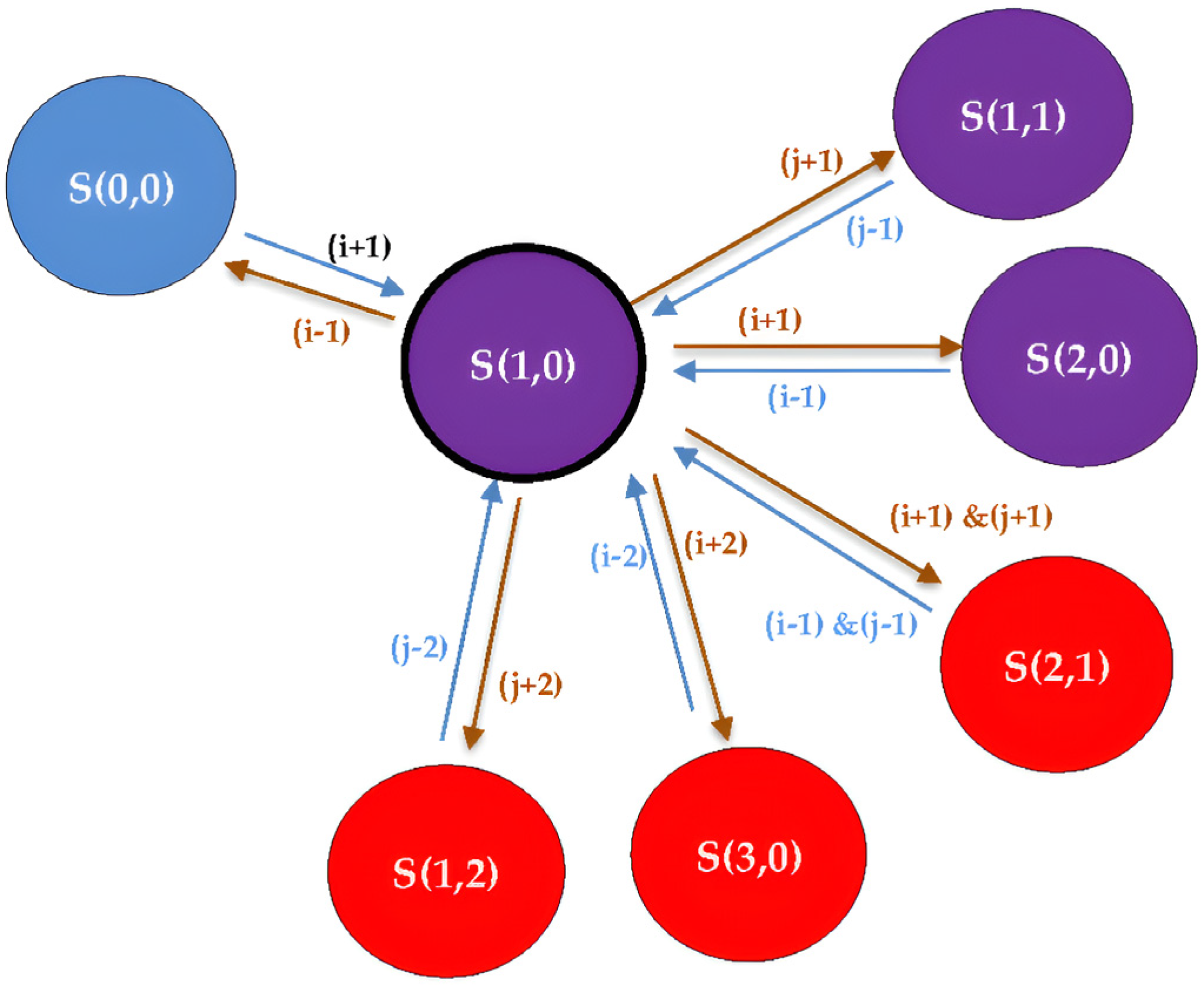
Figure 4.
The transitioning example from S (1,0) in the “Occupied Phase” to the different states in the “Empty Phase” and the “Full Phase”; “S (i,j)” represents different states where “i” is the number of ongoing M2M services and “j” is the number of ongoing H2H services.
Figure 4.
The transitioning example from S (1,0) in the “Occupied Phase” to the different states in the “Empty Phase” and the “Full Phase”; “S (i,j)” represents different states where “i” is the number of ongoing M2M services and “j” is the number of ongoing H2H services.
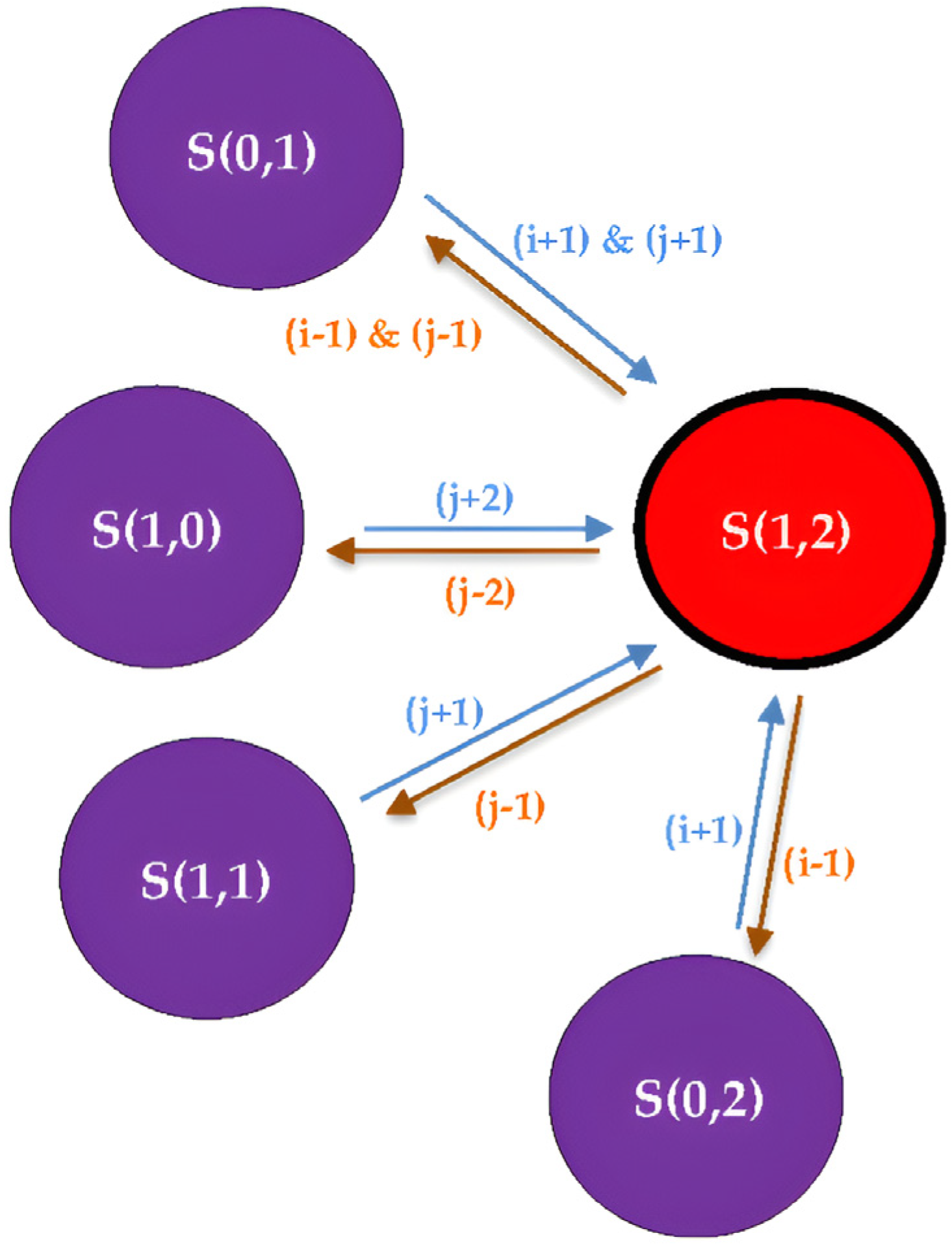
Figure 5.
The transitioning example from S (1,2) in the “Full Phase” to the different states in the “Occupied Phase”; “S (i,j)” represents different states where “i” is the number of ongoing M2M services and “j” is the number of ongoing H2H services.
Figure 5.
The transitioning example from S (1,2) in the “Full Phase” to the different states in the “Occupied Phase”; “S (i,j)” represents different states where “i” is the number of ongoing M2M services and “j” is the number of ongoing H2H services.
Figure 6.
Normal-cycle scenario results, where: S (0,0) represent the initial state, S (0,1) represents one H2H request only, S (0,2) is the state with two H2H requests, and S (0,3) represents three H2H requests, while S (1,0) represents one M2M request only, S (2,0) is the state with two M2M requests, and S (3,0) represents three M2M requests. Moreover, S (1,1) is the state that contains one M2M request and one H2H request, S (1,2) represents the arrival of one M2M request and two H2H requests, and S (2,1) represents the arrival of two M2M requests and one H2H reque.
Figure 7.
The dense-area scenario results, where S (0,0) represents the initial state, S (0,1) represents one H2H request only, S (0,2) is the state with two H2H requests, and S (0,3) represents three H2H requests, while S (1,0) represents one M2M request only, S (2,0) is the state with two M2M requests, and S (3,0) represents three M2M requests. Moreover, S (1,1) is the state that contains one M2M request and one H2H request, S (1,2) represents the arrival of one M2M request and two H2H requests, and S (2,1) represents the arrival of two M2M requests and one H2H request.
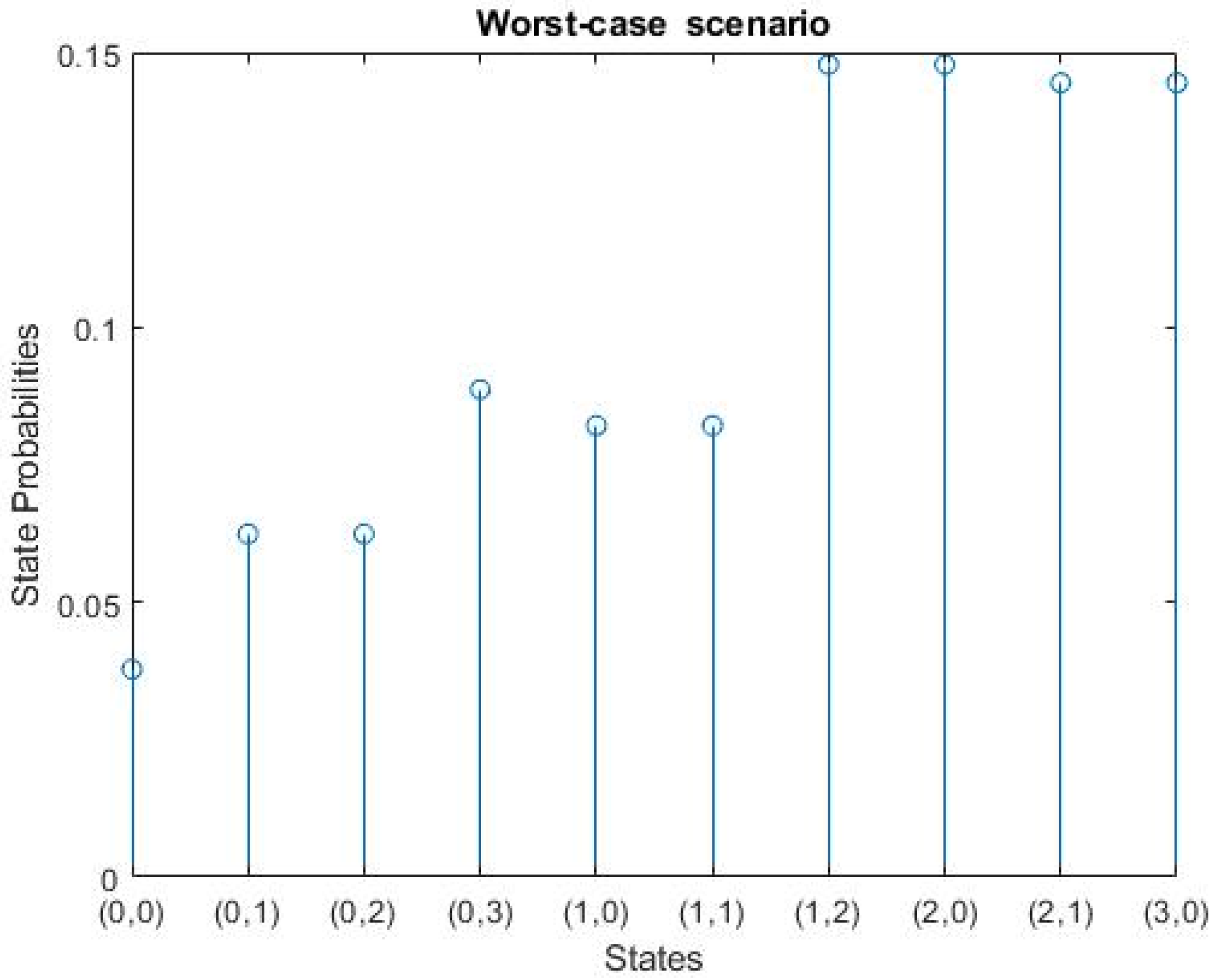
Figure 8.
The worst-case scenario results, where S (0,0) represents the initial state, S (0,1) represents one H2H request only, S (0,2) is the state with two H2H requests, and S (0,3) represents three H2H requests, while S (1,0) represents one M2M request only, S (2,0) is the state with two M2M requests, and S (3,0) represents three M2M requests. Moreover, S (1,1) is the state that contains one M2M request and one H2H request, S (1,2) represents the arrival of one M2M request and two H2H requests, and S (2,1) represents the arrival of two M2M requests and one H2H request.
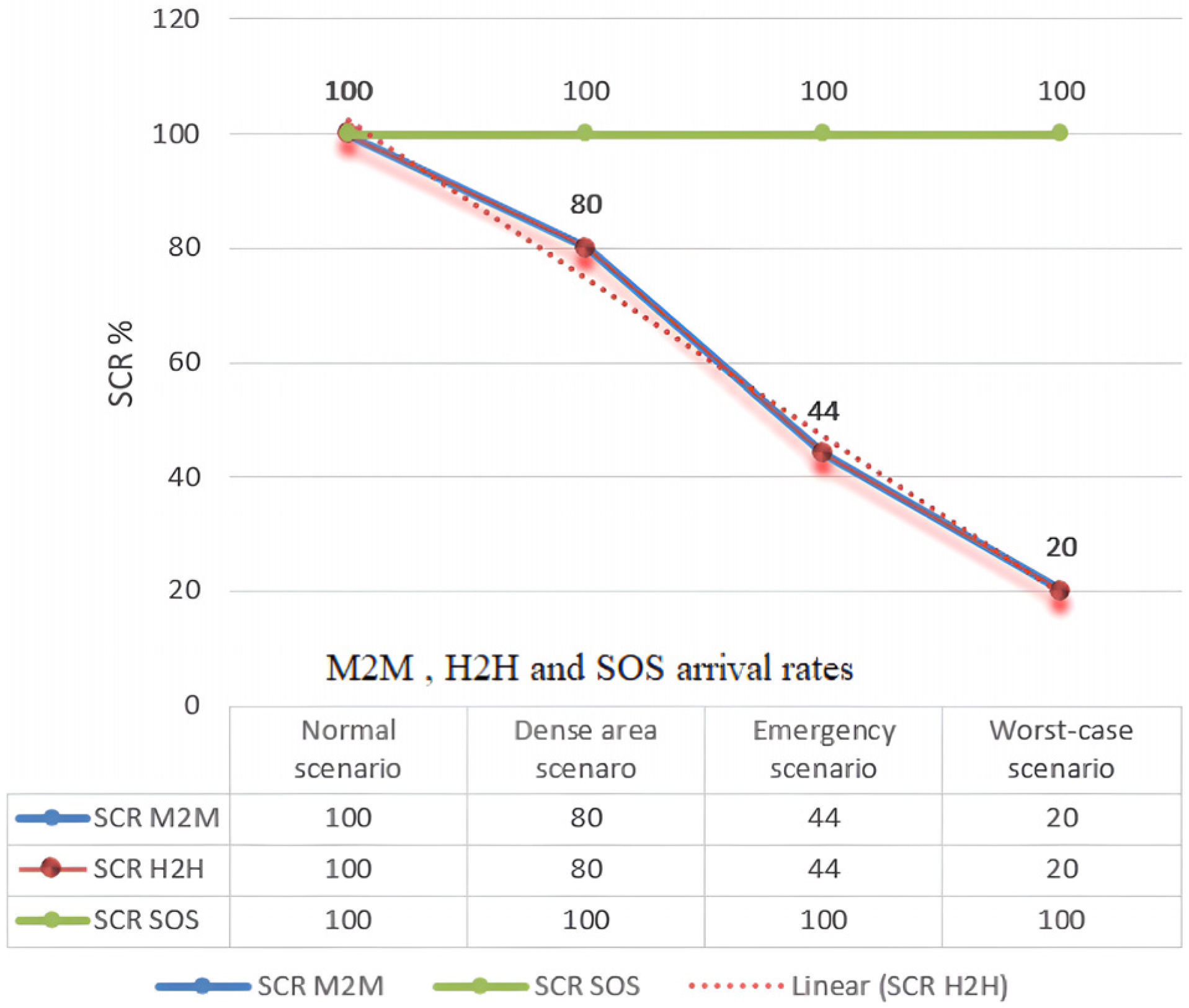
Figure 9.
The impact of the M2M and SOS traffic on the H2H traffic in the different scenarios.
Figure 9.
The impact of the M2M and SOS traffic on the H2H traffic in the different scenarios.
Figure 10.
Impact of H2H and SOS traffic on M2M traffic in different scenarios.
Figure 10.
Impact of H2H and SOS traffic on M2M traffic in different scenarios.
Table 1.
Symbols, notations, values and descriptions.
Table 1.
Symbols, notations, values and descriptions.
| Symbol | Value | Description |
|---|
| C | 3 | Number of resource blocks available in network |
| i | | Number of ongoing M2M services |
| j | | Number of ongoing H2H services |
| λM2M | +1 or +2 | M2M Average arrival rate |
| λH2H | +1 or +2 | H2H Average arrival rate |
| λSOS | +1 & +1 | One M2M request and one H2H request (i + 1 & j + 1) |
| μM2M | −1 or −2 | M2M service rate |
| μH2H | −1 or −2 | H2H service rate |
| μSOS | −1 & −1 | Completion of one M2M request and one H2H request (i − 1 & j − 1) |
| S (i,j) | | State with certain i&j requests |
| π(i,j) | | Steady-state probability |
| п | | Steady-state probability vector |
Table 2.
SCR of H2H, M2M and SOS during normal-cycle scenario.
Table 2.
SCR of H2H, M2M and SOS during normal-cycle scenario.
| Traffic | Departed | Arrived | SCR |
|---|
| M2M | 10,000 | 10,000 | 100% |
| H2H | 5000 | 5000 | 100% |
| SOS | 10,000 | 10,000 | 100% |
Table 3.
SCR of H2H, SOS and M2M for dense-area scenario.
Table 3.
SCR of H2H, SOS and M2M for dense-area scenario.
| Traffic | Departed | Arrived | SCR |
|---|
| M2M | 12,000 | 95,000 | 80% |
| H2H | 5000 | 4000 | 80% |
| SOS | 12,000 | 12,000 | 100% |
Table 4.
SCR of H2H, SOS and M2M for emergency-case scenario.
Table 4.
SCR of H2H, SOS and M2M for emergency-case scenario.
| Traffic | Departed | Arrived | SCR |
|---|
| M2M | 16,000 | 68,000 | 44% |
| H2H | 5000 | 22,000 | 44% |
| SOS | 16,000 | 16,000 | 100% |
Table 5.
SCR of H2H, SOS and M2M for worst-case scenario.
Table 5.
SCR of H2H, SOS and M2M for worst-case scenario.
| Traffic | Departed | Arrived | SCR |
|---|
| M2M | 20,000 | 4000 | 20% |
| H2H | 5000 | 1000 | 20% |
| SOS | 20,000 | 20,000 | 100% |
Table 6.
SCR of H2H, SOS and M2M for normal-cycle scenario.
Table 6.
SCR of H2H, SOS and M2M for normal-cycle scenario.
| Traffic | Departed | Arrived | SCR |
|---|
| M2M | 5000 | 5000 | 100% |
| H2H | 10,000 | 10,000 | 100% |
| SOS | 10,000 | 10,000 | 100% |
Table 7.
SCR of H2H, SOS and M2M for dense-area scenario.
Table 7.
SCR of H2H, SOS and M2M for dense-area scenario.
| Traffic | Departed | Arrived | SCR |
|---|
| M2M | 5000 | 4000 | 80% |
| H2H | 12,000 | 9500 | 80% |
| SOS | 12,000 | 12,000 | 100% |
Table 8.
SCR of H2H, SOS and M2M for emergency-case scenario.
Table 8.
SCR of H2H, SOS and M2M for emergency-case scenario.
| Traffic | Departed | Arrived | SCR |
|---|
| M2M | 5000 | 2000 | 44% |
| H2H | 16,000 | 7000 | 44% |
| SOS | 16,000 | 16,000 | 100% |
Table 9.
SCR of H2H, SOS and M2M for worst-case scenario.
Table 9.
SCR of H2H, SOS and M2M for worst-case scenario.
| Traffic | Departed | Arrived | SCR |
|---|
| M2M | 5000 | 1000 | 20% |
| H2H | 20,000 | 4000 | 20% |
| SOS | 20,000 | 20,000 | 100% |


