Article

Tool Condition Monitoring in the Milling Process Using Deep Learning and Reinforcement Learning

by
Devarajan Kaliyannan
1,
Mohanraj Thangamuthu
1,*,
Pavan Pradeep
1,
Sakthivel Gnansekaran
2,
Jegadeeshwaran Rakkiyannan
3 and
Alokesh Pramanik
4
1
Department of Mechanical Engineering, Amrita School of Engineering, Amrita Vishwa Vidyapeetham, Coimbatore 641112, India
2
School of Mechanical Engineering, Vellore Institute of Technology, Chennai 600127, India
3
Centre for Automation, School of Mechanical Engineering, Vellore Institute of Technology, Chennai 600127, India
4
School of Civil and Mechanical Engineering, Curtin University, Perth 6102, Australia
*
Author to whom correspondence should be addressed.
J. Sens. Actuator Netw. 2024, 13(4), 42; https://doi.org/10.3390/jsan13040042
Submission received: 1 July 2024 / Revised: 24 July 2024 / Accepted: 26 July 2024 / Published: 30 July 2024
(This article belongs to the Special Issue Fault Diagnosis in the Internet of Things Applications)

Abstract

:
Tool condition monitoring (TCM) is crucial in the machining process to confirm product quality as well as process efficiency and minimize downtime. Traditional methods for TCM, while effective to a degree, often fall short in real-time adaptability and predictive accuracy. This research work aims to advance the state-of-the-art methods in predictive maintenance for TCM and improve tool performance and reliability during the milling process. The present work investigates the application of Deep Learning (DL) and Reinforcement Learning (RL) techniques to monitor tool conditions in milling operations. DL models, including Long Short-Term Memory (LSTM) networks, Feed Forward Neural Networks (FFNN), and RL models, including Q-learning and SARSA, are employed to classify tool conditions from the vibration sensor. The performance of the selected DL and RL algorithms is evaluated through performance metrics like confusion matrix, recall, precision, F1 score, and Receiver Operating Characteristics (ROC) curves. The results revealed that RL based on SARSA outperformed other algorithms. The overall classification accuracies for LSTM, FFNN, Q-learning, and SARSA were 94.85%, 98.16%, 98.50%, and 98.66%, respectively. In regard to predicting tool conditions accurately and thereby enhancing overall process efficiency, SARSA showed the best performance, followed by Q-learning, FFNN, and LSTM. This work contributes to the advancement of TCM systems, highlighting the potential of DL and RL techniques to revolutionize manufacturing processes in the era of Industry 5.0.

1. Introduction

The cutting tool is in contact with the workpiece during the machining process, and the degree of wear will have a direct influence on the quality of the machining process. Making changes to the tool based on personal experience will always result in poor judgment. Early tool replacement will lower the tool’s utilization rate and raise production costs. If the tool is not changed promptly, the workpiece’s surface quality will quickly deteriorate, resulting in the creation of unqualified products. Acute tool wear can lead to chatter, chipping, and tool fractures, as well as harm to the machine tool and operator. Hence, it is crucial to keep an eye on the tool’s condition during actual machining to minimize unnecessary downtime and the processing costs brought on by tool wear [1,2]. Tool Condition Monitoring systems (TCMs) in the manufacturing sector have been increasingly favored to mitigate the expenses linked to tool wear and failure. Twenty percent of machine tool downtime is caused by tool failure, indicating that tool wear affects the precision and quality of the machined surface, as well as equipment efficiency [3].
TCMs with high accuracy are crucial for raising machine part quality and productivity. In light of this perspective, a substantial quantity of research in the field of TCMs is being conducted globally [4]. Direct and indirect monitoring are the two major classes of cutting tool monitoring techniques [2]. Since indirect approaches are more flexible than direct methods, they have become very popular. Vibration signals [4,5,6], cutting force [7,8], acoustic emission (AE) [7], spindle motor current [9], cutting zone temperature [10], vision system [11], and machined surface images [12] are some of the commonly used indirect monitoring signals. TCMs are essential to contemporary manufacturing procedures, particularly for tasks requiring a high degree of precision, like milling. Through cost reductions and productivity increases, they offer considerable economic advantages in addition to fostering sustainability and ongoing development. TCMs play a crucial role in attaining operational excellence and competitiveness as manufacturing shifts to more sophisticated and intelligent systems.
Many techniques, including data-driven/statistical models and physics-based models, have been developed to accurately predict tool wear. Physics-based models need a thorough understanding of the system to create models based on the essential failure mechanisms. Because of the wear process’s complexity and a lack of complete understanding, accurate analytical models are uncommon and, as a result, have a limited scope and set of applications. For the models to be trained, data-driven models need a large amount of data, but they do not require much process expertise [13,14]. Machine Learning (ML) algorithms are used for classification and regression problems [15].
A TCM for end milling was developed through the extraction of Hoelder’s Exponent (HE) characteristics from vibration signatures with various Machine Learning (ML) algorithms, and it was found that the Support Vector Machine (SVM) and Decision Tree (DT) with HE and wavelet features yielded better classification accuracies of 99.86% and 100%, respectively [5]. Vibration signals were processed to extract statistical characteristics like variance, skewness, kurtosis, and mean [16]. A detailed review of Deep Learning (DL) architectures and frameworks was reviewed [17]. The milling process employed a Convolutional Long Short-Term Memory Network (ConvLSTM) to monitor the condition of the tool. ConvLSTM combines the benefits of Convolutional Neural Network (CNN) local characteristic extraction with the sequential modeling capability of LSTM to better accomplish the anticipation task by substituting the convolution operation for the matrix product in the LSTM cell [18]. CNN models are used for image classification problems [19] and surface profile classification [20].
A TCM for the milling process was developed with vibration and cutting force signals using a Deep Belief Network (DBN) and yielded a classification accuracy of 99% [21]. To develop the online TCMs, Dou et al. [22] gathered the cutting force and vibration signals during the milling process and built a Sparse Auto-Encoder (SAE). Cai et al. [23] employed stacked LSTM networks to gather deep features from NASA and PHM datasets. The statistical, frequency, and time–frequency domain features were fed into a nonlinear regression model to track the tool condition. Various ML models like Linear Regression (LR), Support Vector Regression (SVR), Multi-Layer Perceptron (MLP), CNN, and LSTM were applied, and LSTM yielded the highest accuracies of 97.85% and 90.06% for the 2010 PHM and NASA data sets, respectively.
Ou et al. [24] applied Gaussian kernel functions to augment the attribute learning capability of the novel Deep Kernel Auto-Encoder (DKAE) optimized with Gray Wolf Optimizer (GWO) to monitor the milling tool condition. The three-axis motor current was considered an input feature, and various other ML models were employed to estimate the performance of the suggested model. The results revealed that the suggested model enhanced accuracy by 8% compared to the baseline ML models. Along with DL models, transformers also have a significant role in classification problems [25]. Transfer learning (TL) has a significant effect on TCM. The Inception-V3 with TL model yielded a maximum accuracy of 99.4% to predict the tool wear with images [26].
Liu et al. [27] employed Fully Connected Networks (FCN) to predict tool conditions, Parallel Residual Networks (PRes), and stacked bidirectional LSTM networks (PRes–SBiLSTM) to extract features from AE, cutting force, and vibration signals. The proposed algorithm was compared with LR, SVR, Residual Network (ResNet), ResNet and a Stacked Bidirectional LSTM (ResNet–SBiLSTM), and Parallel CNN and SBiLSTM (PCNN–SBiLSTM) and found that the proposed model performed better than the baseline models. Chen et al. [28] combined an AE signal with tool images to monitor tool conditions during milling operations. They mapped the wear quantity taken from the vision camera with the attributes of the AE and used ML techniques like BPNN and SVM. The proposed method yielded an accuracy of 96.11%.
A deep CNN was used to extract attributes to afford automatic online TCM [29]. Nguyen et al. [30] introduced a DL model with Stacked Auto-Encoders (SAE) to recognize tool conditions during the machining of cast iron. The SAE model recognized different tool conditions with high accuracy and achieved high classification accuracy. Ma et al. [31] created a DL model to predict the tool wear using force signals during titanium alloy milling by combining two CNN + BiLSTM and a CNN Bi-Directional Gated Recurrent Unit (CNN + BiGRU) models. The proposed model performed better than other DL models, with an error of 8%.
Various research work has been carried out to predict tool wear and classify tool conditions using ML and DL models with various features like time, frequency, and time–frequency domain. To the best of the authors’ knowledge, the implementation of TCM with Reinforcement Learning (RL) was not explored further. RL offers a powerful framework for addressing dynamic decision-making problems in TCM. By leveraging RL, TCM systems can continuously learn and adapt to changing conditions, optimizing tool usage and process parameters in real time. The objective is to explore the performance of RL in TCM applications and compare the results with DL algorithms. The research questions addressed in this work are as follows:
  • RQ1: Study the effect of tool wear on vibration signals.
  • RQ2: Analyze the performance of DL and RL for TCM applications.

2. Materials and Methods

2.1. Workpiece Material

The workpiece, which had measurements of 100 × 50 × 50 mm, was designated as “Mild steel” for the face milling process. For the operation, mild steel of the ASTM A36 grade was employed. Due to its low cost, high force resistance, and suitability for various machining methods, mild steel was chosen as the workpiece. Additionally, due to these qualities, mild steel is the most commonly used workpiece [32].

2.2. Cutting Tools

Face milling is a type of machining process that involves using a CNC milling machine. The Gaurav BMV 35 series CNC milling machine was used. A tungsten carbide tool was utilized in this face milling operation (Mitsubishi Materials, Tokyo, Japan SEMTI3T3AGSN-IM VPISTF). The face-milling cutter had four flutes. The face-milling process was carried out with optimal parameters of 2600 RPM spindle speed, 130 mm/min feed rate, and 1.5 mm depth of cut with commercial cutting fluid. Three different tools with different wear lands were used. The tools were designated as “New”, “working” (less than 0.2 mm wear), and “dull” (greater than 0.3 mm wear). The machining setup used is presented in Figure 1.

2.3. Measurement

An Arduino-based Data Acquisition System (DAQ) is integrated into a TCM. The code in the Arduino IDE uses an Adafruit library to record acceleration in the x, y, and z axes. Utilizing an MPU 6050 accelerometer (TDK InvenSense, San Jose, CA, USA), the vibration signal is recorded. There is a sequential mention of the circuit connection between the MPU 6050 Accelerometer and the Arduino Uno Rev 3 (Make: Arduino, Torino, Italy, Controller: ATmega328P, Microchip Technology, Chandler, AZ, USA). Analog pin A5 (Arduino)—SCL (MPU6050 Accelerometer), Analog pin A4 (Arduino)—SCA, GND (Arduino)—GND (MPU6050 Accelerometer), and 5 V input (Arduino)—VCC (MPU6050 Accelerometer) are the connections that are made using jumper cables. The MPU6050 sensor is calibrated to negate the slag value once it is fixed in the spindle of the CNC machine.

2.4. Decision-Making Algorithm

Decision-making algorithms are crucial for implementing effective TCMs in manufacturing. These algorithms analyze data from sensors and make decisions about the tool conditions. From simple rule-based systems to advanced reinforcement learning techniques, each approach has its advantages and challenges. By selecting and combining the appropriate algorithms, TCMs can be designed to provide accurate real-time monitoring and decision-making, leading to optimized tool usage, reduced downtime, and enhanced product quality. In this work, DL and RL algorithms were used for predicting the tool condition.

2.5. Deep Learning (DL)

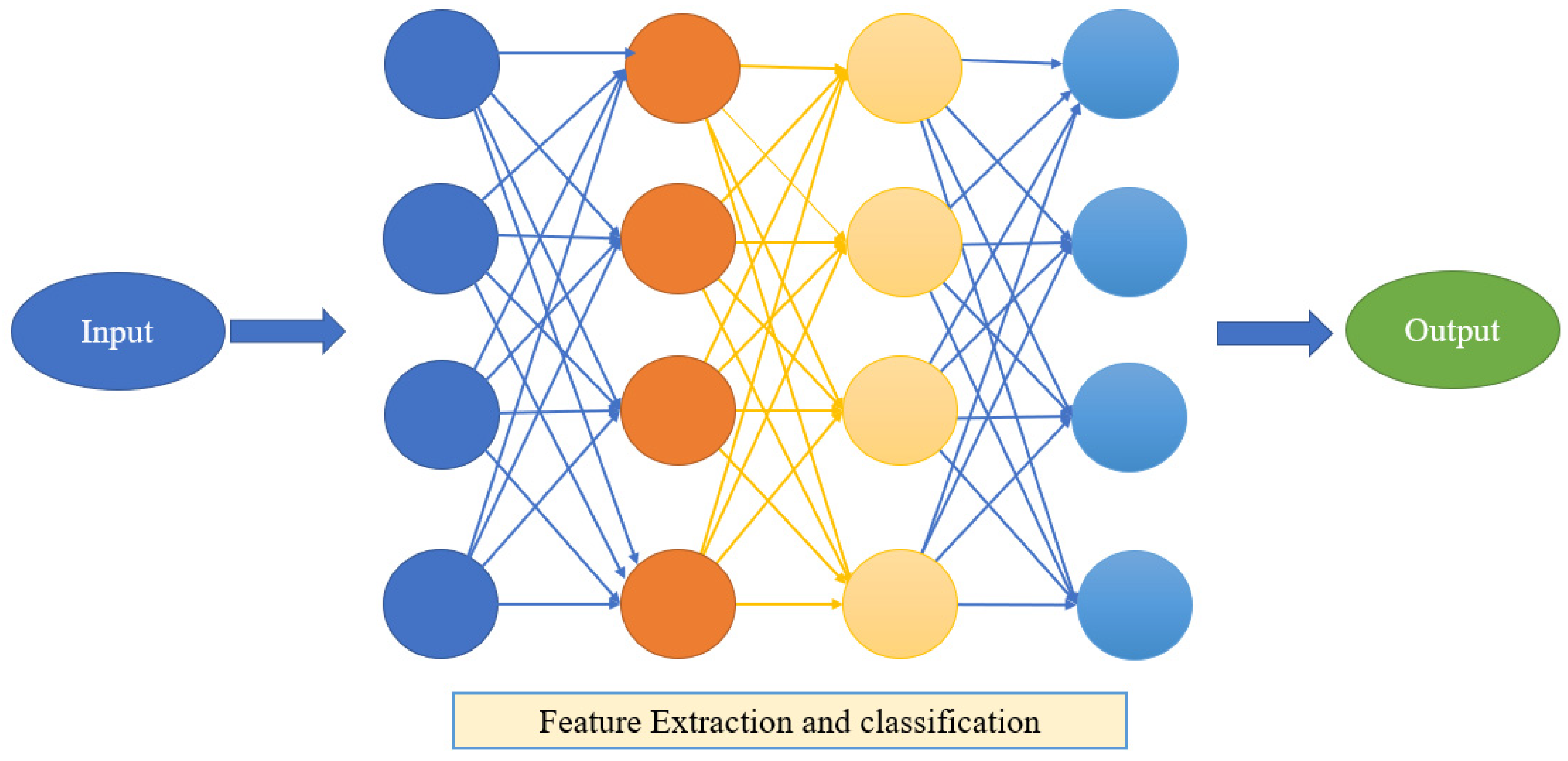
A form of machine learning called DL uses multiple-layered neural networks to learn from and extract features from vast volumes of data. Furthermore, it is anticipated that tool condition and process monitoring will be among the possible manufacturing domains where DL will find applications. As opposed to conventional machine learning methods, DL has the potential to automatically learn complicated and hierarchical representations of data, which can result in more accurate predictions and improved performance. Figure 2 represents the architecture of the DL model.

2.6. Long Short-Term Memory (LSTM)

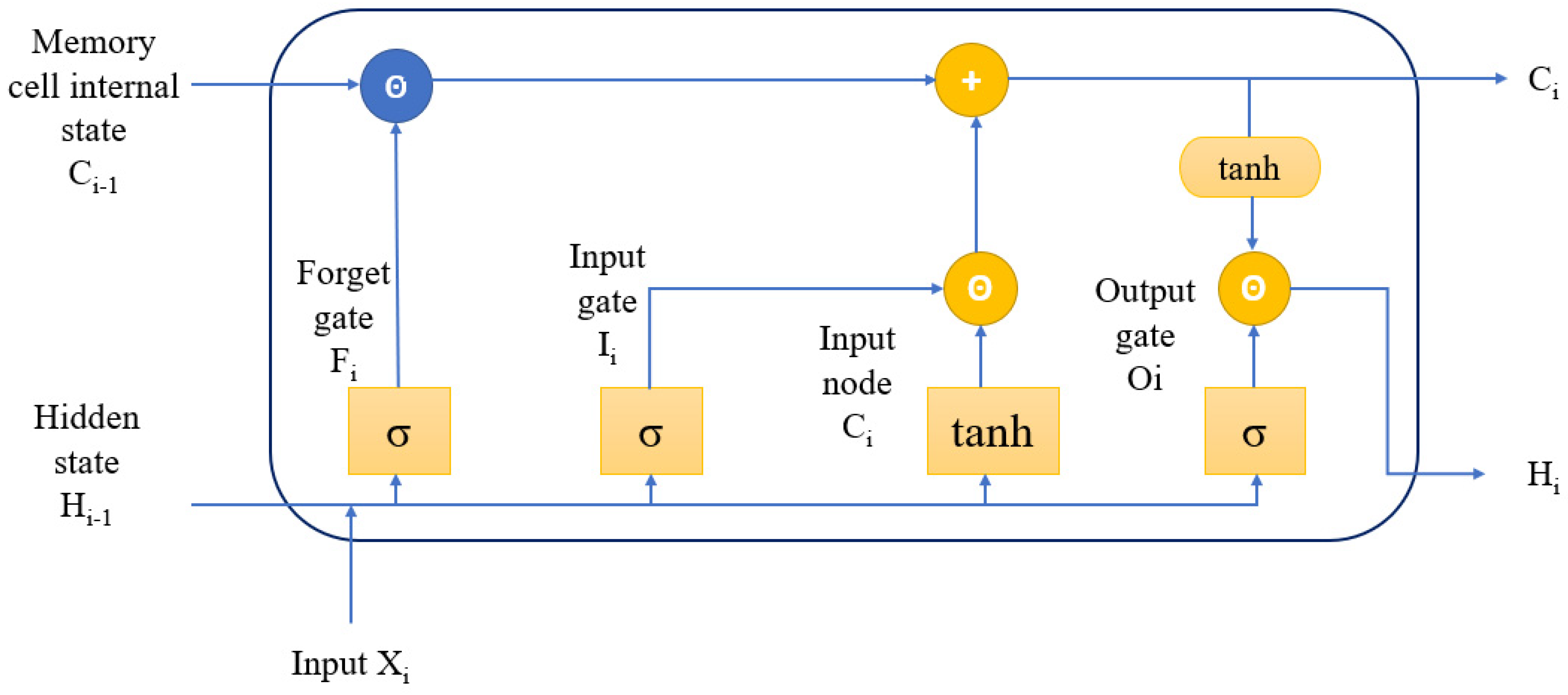
Long Short-Term Memory (LSTM) is a kind of Recurrent Neural Network (RNN) model that is extensively employed for prediction tasks, and it is designed to overcome the hurdles of traditional RNNs, particularly the vanishing and exploding gradient problems and a restricted capacity to recall long-term requirements. The core of LSTM architecture is its memory cell, which can preserve its state over time, and three gates, the input, the forget, and the output gates, regulate the flow of data into and out of the cell. The cell state is the memory of the network. It carries information across the entire sequence processing and can be modified by the various gates. The hidden state is the output of the LSTM unit at each time step. It is used for the final output of the sequence processing and influences the cell state updates. The architecture of the LSTM model is illustrated in Figure 3.
The input gate establishes whether the data from the previous timestamp should be saved in memory or if it is irrelevant and can be disregarded. The input to this cell is where the forget gate looks for new information. The updated information from the present timestamp is finally passed to the succeeding timestamp by the output gate. As illustrated in Figure 3, the input at the present step and the hidden state of the preceding time step are fed into the LSTM gates. For the input gate, forget gate, and output gate, three fully connected (FC) layers with sigmoid activation functions calculate their values. All the gate values are within the range of (0, 1) due to the sigmoid activation.

2.7. Feed Forward Neural Network (FFNN)

A group of artificial neural networks known as FFNN evaluates input data and provides predictions using a network of linked layers. A single-layer perceptron is called FFNN. The architecture of FFNN is shown in Figure 4. A sequence of inputs is fed into the layer and multiplied by the weights of the model. The total is computed by totaling the weighted input values. The output layer generates the final predictions, whereas the input layer gets the data from the input source. The output value is 1 if the sum of the values goes beyond a set value, which is normally set at 0, and −1 if the sum is less than the set value. Backpropagation is a technique for training FFNNs that entails changing the network’s weights to reduce the difference between the expected and actual output. An FFNN is an architecture where data move in one direction, moving from the input layer via hidden layers until reaching the output layer. There are no feedback connections in this network. In this study, the architecture consists of FC layers, where each neuron is linked to all neurons in the previous and following layers. This type of network is commonly employed for classification tasks, as it learns to associate input features with class labels by adjusting weights and biases during training.

2.8. Reinforcement Learning (RL)

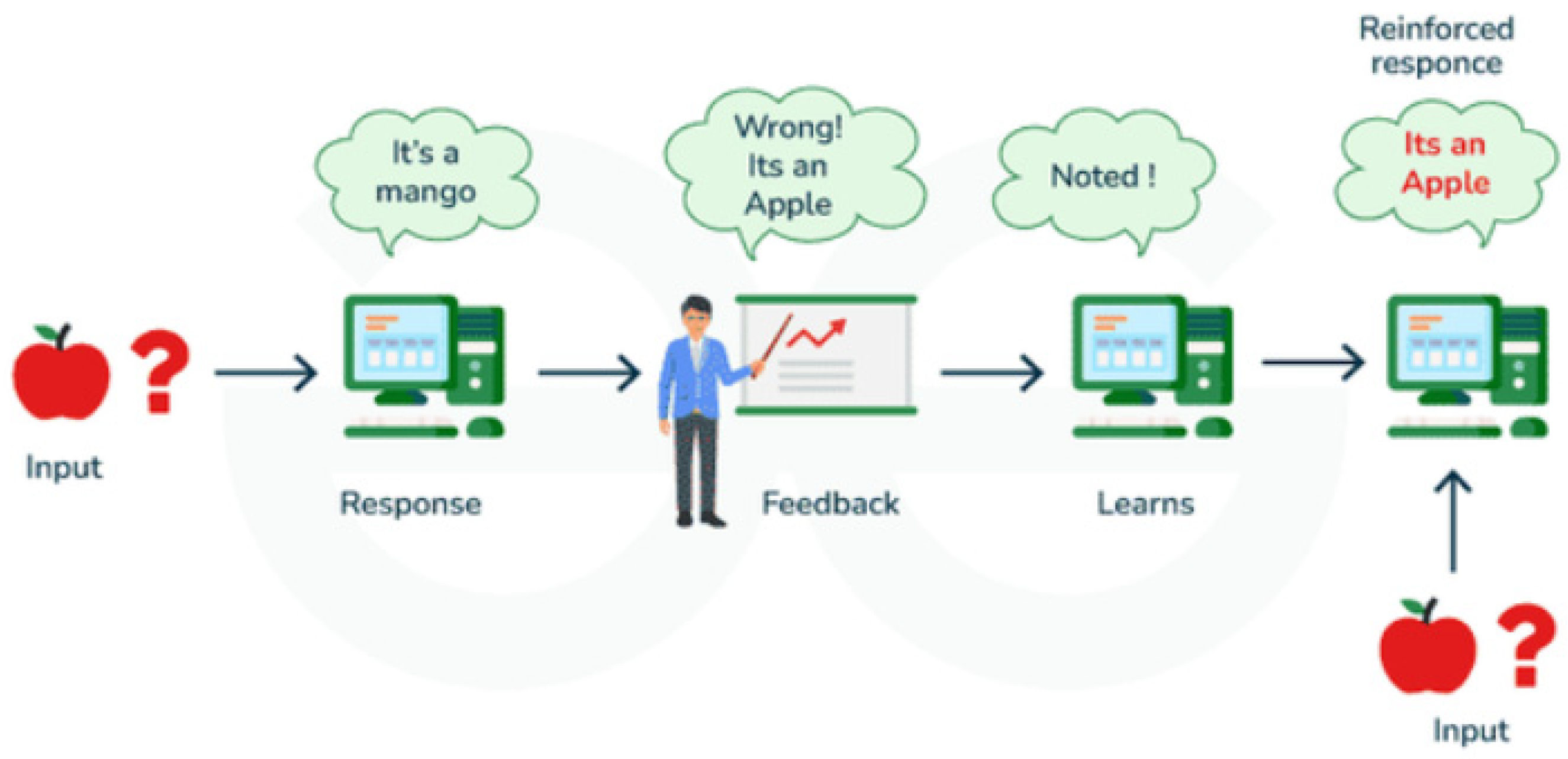
A type of ML called RL trains an agent how to function in a given environment by observing how it is rewarded or punished for its behaviors. RL aims to discover the best policy to expand the forecasted reward over time. Model-based and model-free RL algorithms are the two basic subtypes [33]. While model-free algorithms learn directly from experience without a model, model-based algorithms employ a model of the environment to anticipate the effect of an action. The block diagram for RL is presented in Figure 5. There are five fundamental components to the RL approach [34].
An agent interacts with its surroundings after being trained by a goal-oriented algorithm.
A state, represented by the symbol “st”, is the data gathered from the surroundings.
An award is represented by the symbol “rt” and is the result of an agent’s interaction with the environment, either positive or negative.
A behavior is an agent’s manner of moving that is expressed as “at” and is determined by the information they have gathered from their surroundings.
The agent observes the given environment.
By tuning a model’s parameters depending on input from the environment, reinforcement learning may be used to increase the accuracy of predictions. For instance, in a speech recognition system, the agent can be trained to modify the neural network’s weights to increase the recognition accuracy of the speech. To increase the model’s accuracy, reinforcement learning may also be used to optimize hyperparameters like learning rates and regularization parameters. The precision of predictions can be increased with less manual adjustment and monitoring by utilizing RL.

2.9. Q-Learning

Q-learning is a type of RL algorithm, which is a model-free algorithm and an off-policy algorithm that estimates the optimum action-value function Q (s, a) of an agent, which represents the anticipated long-term reward for standing a given action in a given state. The block diagram for Q-learning is shown in Figure 6. During the training process, the agent cooperates with the environment by pleasing actions and obtaining rewards. It uses the Bellman equation to update its Q-values based on the performed rewards and switches between states and actions. The agent learns to select actions that maximize the anticipated long-term reward, which is determined by the Q-values. By iteratively applying the Bellman equation, the Q-values eventually converge to the optimal values.

2.10. SARSA

For resolving Markov decision processes, reinforcement learning is employed with the SARSA algorithm. The acronym “SARSA” stands for the algorithm’s update of its Q-values through the use of the tuple (state, action, reward, next state, next action). It adopts an “on-policy” strategy (epsilon-greedy), which suggests that it educates itself on how the policy being implemented will promote environmental interactions [35]. According to the information the agent has learned from interacting with the environment, the SARSA technique continuously modifies its Q-value estimations. The program uses an epsilon-greedy technique, in which the agent selects the action with the larger value of Q with a probability of 1, epsilon, and a random action with a probability of striking an equilibrium between operation and searching.
Prediction accuracy, which includes estimating how well a model will perform on data that has not yet been observed, is a fundamental machine learning challenge. SARSA can be used to estimate a model’s accuracy by training it on a subset of the data and then testing it on an unseen data set. The algorithm can discover the relationship between the attributes and the target to assess the model’s accuracy on new data. SARSA can be integrated with other methods, such as gradient boosting or neural networks, to improve prediction accuracy. By estimating a model’s accuracy, researchers and practitioners can assess whether it is suitable for a certain task and can identify areas that need improvement.

2.11. Performance Metrics

The performance metrics are crucial for estimating the efficiency of the model [36]. The metrics used in this work are given below.
Confusion Matrix: A table that describes the performance of the ML model by displaying the values of True Positives (TP), True Negatives (TN), False Positives (FP), and False Negatives (FN).
FP: No. of negative cases incorrectly categorized as positive.
TN: No. of negative cases correctly categorized as negative.
TP: No. of positive cases correctly categorized as positive.
FN: No. of positive cases incorrectly categorized as negative.
Precision: It evaluates the accuracy of the correct predictions.
Pr e c i s i o n = T P T P + F P
Recall: It determines the ability of the model to find all the relevant cases. It is also called “True Positive Rate” (TPR) or Sensitivity.
Re c a l l = T P T P + F N
Accuracy: It represents the percentage of properly categorized cases out of the total number of cases.
A c c u r a c y = N o .   o f   c o r r e c t   p r e d i c t i o n s T o t a l   N o .   o f   p r e d i c t i o n s
False Positive Rate (FPR): It indicates the percentage of negative cases that are incorrectly categorized as positive. In other words, it measures how often the model incorrectly predicts the positive class. A lower FPR indicates a better performance in terms of minimizing misclassification.
F P R = F P F P + T N
F1 Score: It is the harmonic mean of Precision and Recall, providing stability between the two.
F 1   S c o r e = 2 × Pr e c i s i o n × Re c a l l Pr e c i s i o n + Re c a l l
ROC Curve (Receiver Operating Characteristic Curve): A graph showing the performance of a classification model at all classification thresholds. It plots the Recall against the FPR.

3. Results and Discussion

3.1. RQ1: Study the Effect of Tool Wear on Vibration Signals

Effect of Flank Wear on Vibration Signals

The nature of the vibration signal starts from the machining process and includes the parts of free, forced, periodic, and random types of vibration. It is difficult to directly measure the vibration signals due to its formative distinctive feature, and the mode of vibration depends on the frequency. Hence, the vibration is measured as an acceleration signal [37].
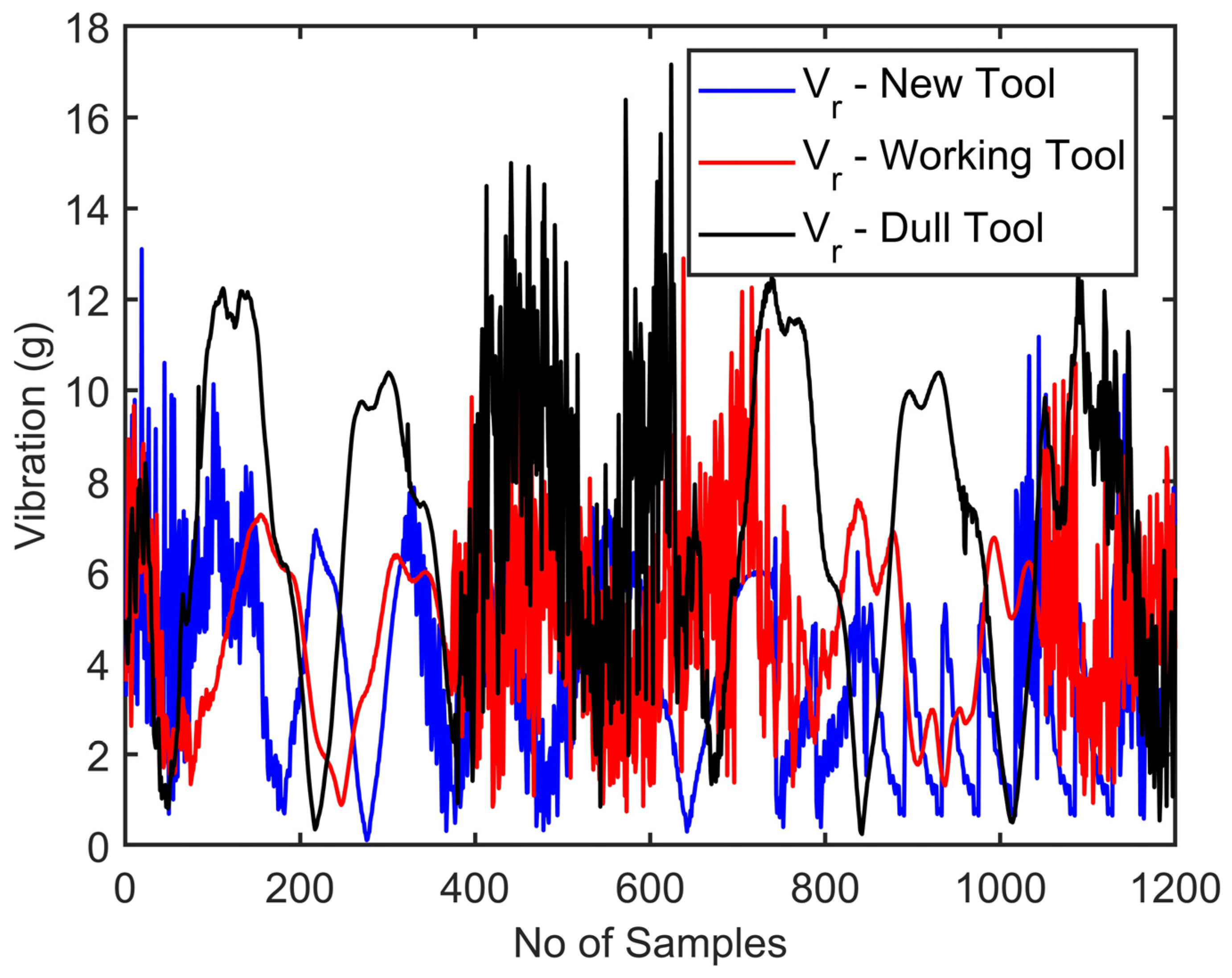
The vibration in the x, y, and z axes was used to estimate resultant vibration (Vr) signals. The Vr signal was employed to predict the cutting tool condition. The Vr signals for cutting tools with different tool conditions are presented in Figure 7. The dull tool had a maximum vibration of 22 g. At the initial stage of the cutting process, the new tool also exhibits significant vibration due to contact with the cutting tool and workpiece. Due to the effect of tool wear, the vibration amplitude was increased [38].
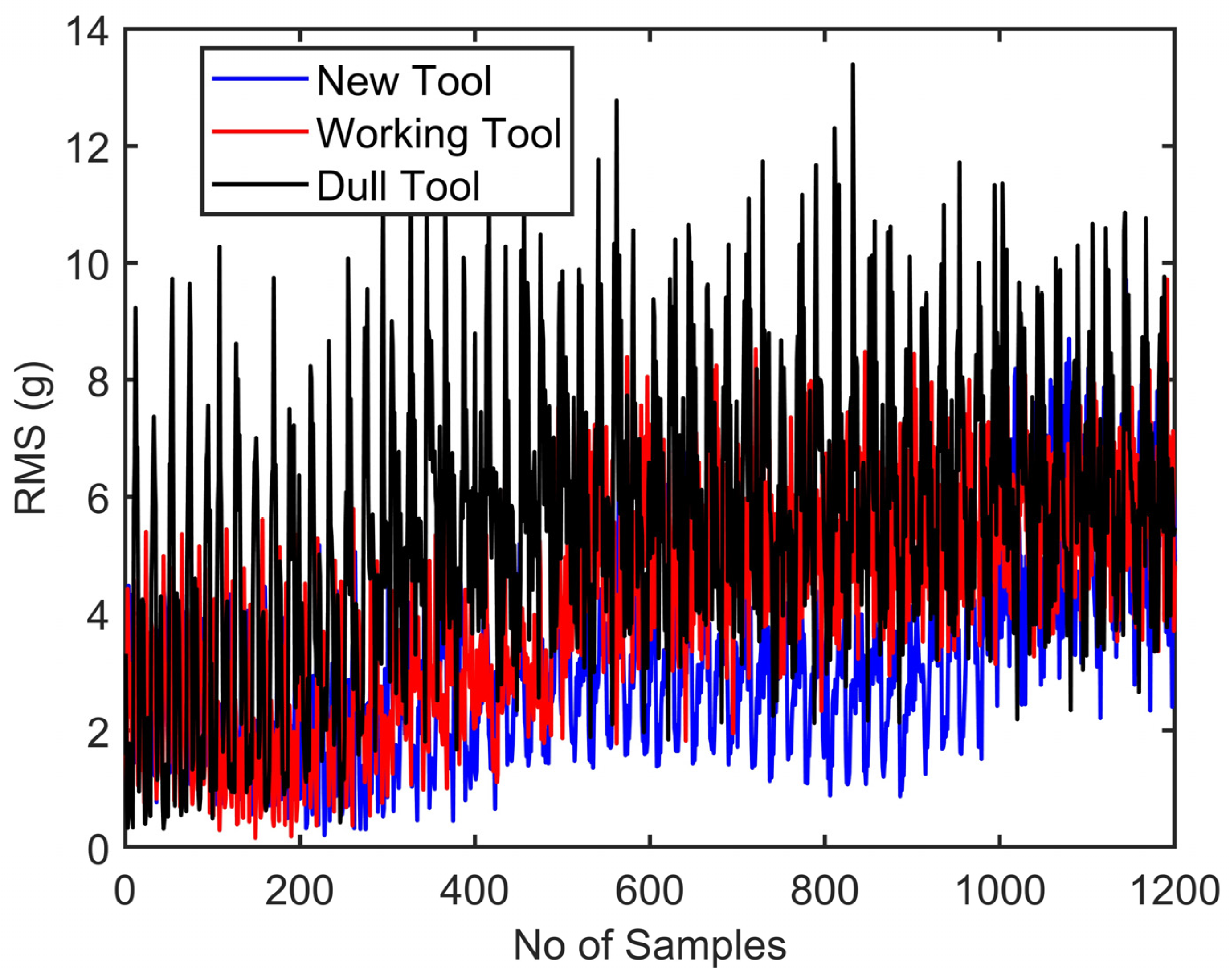
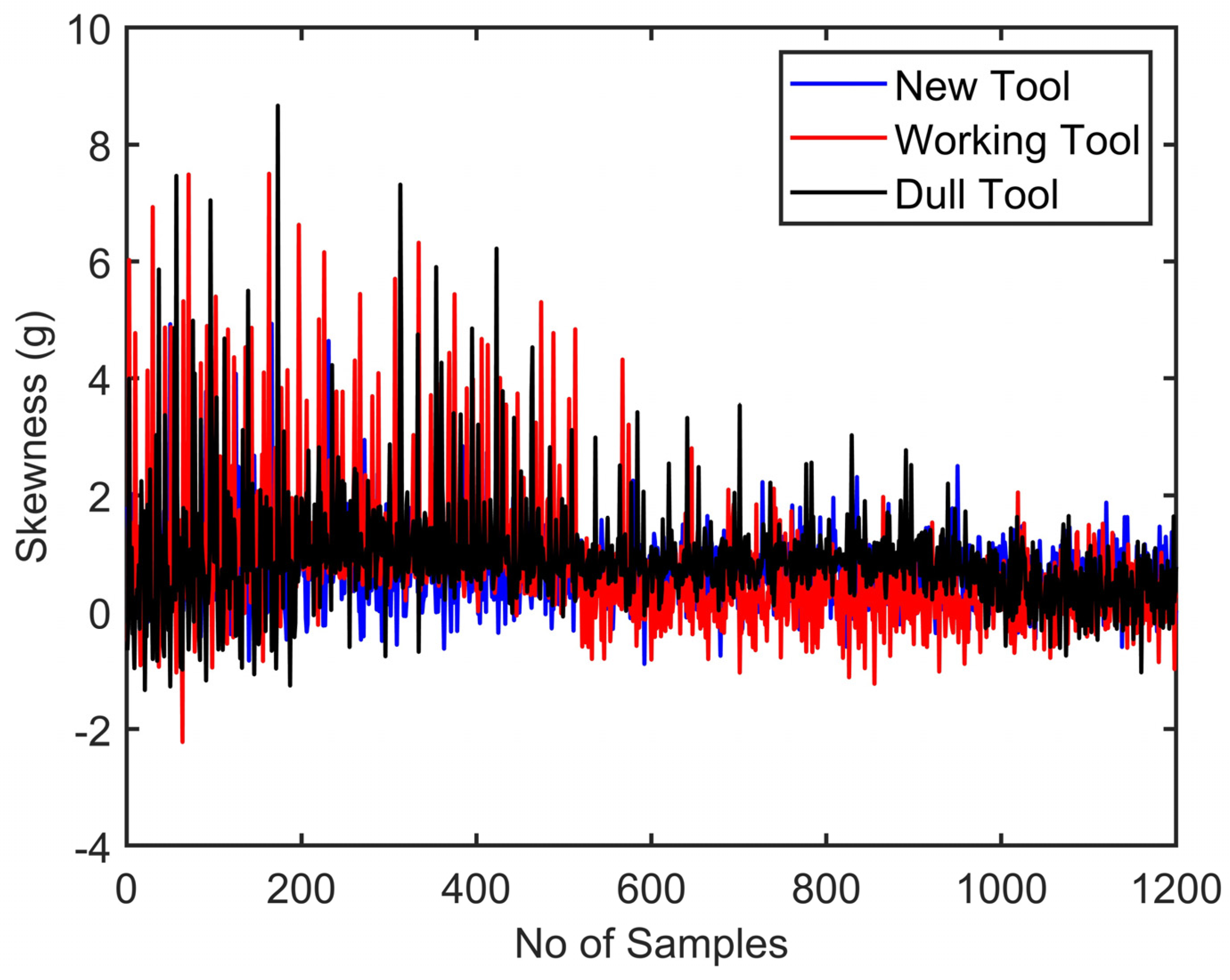
The statistical response of resultant vibration signals is presented in Figure 8, Figure 9 and Figure 10. In all the statistical responses, the amplitude for the dull tool was higher than for the new and working tools. It was identified that time-domain vibration signatures were very sensitive to tool wear. The experimental results proved that the RMS, kurtosis, and skewness values heightened significantly for dull tools. The increase in amplitude for dull tools was found in the literature [39,40]. Also, the same trend was found in the drilling process [41]. When tool wear increased, the acceleration signal in each axis was increased. Hence, the resultant vibration also increased. Due to failed cutting edges, the expanded wear leads to a rise in the contact area between the tool and the workpiece. In general, vibration amplitude increased with an increase in flank wear [42,43].

3.2. RQ2: Analyze the Performance of DL and RL for TCM Applications

3.2.1. TCM Using DL Models

The classification algorithm incorporates an LSTM model, a variant of RNNs. First, the training data is sourced from an Excel file and categorized into three groups. These categories are then merged into a unified dataset. Next, the data is partitioned into training and testing, with 80% assigned for training and the remaining 20% for testing purposes. The training process for the input data involved utilizing a dataset comprising 24,000 data points, categorized into three groups: 800 “new”, 800 “working”, and 800 “dull”. The architecture of the LSTM model is defined, incorporating various layers such as sequence input, LSTM, FC layers, Softmax, and Output layers. Training the model involves utilizing the Adam optimizer and specific training options, including maximum epochs, mini-batch size, shuffling, and validation data. Following training, the model is devoted to anticipating outputs on the test set, and its performance is assessed using accuracy metrics and a confusion matrix [44,45]. For each class, 200 data points were used for testing.
The confusion matrix offers valuable insights into the distribution of predicted labels compared to the true labels. This algorithm effectively showcases the ability of LSTM models to capture sequential dependencies, making them applicable to tasks such as time series analysis or text classification. During the training process, the dataset was fed to the LSTM model, which iteratively learned the patterns and relationships within the input sequences. The learning rate of 0.001 determined the step size for adjusting the model’s internal parameters during training, controlling the rate at which the model adapted to the data. The average accuracy of 94.85% achieved on the test set indicated how well the trained LSTM model generalized to unseen data. This accuracy was attained by configuring the LSTM algorithm with specific parameters, such as a learning rate of 0.001, 100 epochs, and 240 iterations per epoch. This repetitive training allowed the LSTM algorithm to gradually improve its performance by refining its predictions and reducing the overall prediction error. This performance metric serves as a measure of the model’s predictive capability and provides an estimate of its accuracy when deployed in real-world scenarios.
A confusion matrix was generated to validate the obtained results and assess the prediction accuracy of test data. The confusion matrix is depicted in Figure 11 and visually represents the model’s performance. It consists of a tabular layout with three rows and three columns. The values in the confusion matrix represent the number of samples from each category that were correctly or incorrectly classified by the model. In the given confusion matrix, the first row indicates the new category. The model correctly predicted 181 samples as new, while 19 samples from this category were misclassified as working. The second row represents the working category. The model accurately identified 188 samples as working but misclassified 12 samples from this category as new. The third row corresponds to the dull category. All 200 samples from this category were correctly classified as dull. The model’s performance can be evaluated by predicting the different categories by analyzing the confusion matrix. It demonstrates that the model achieved high accuracy in classifying the dull category, while it had a higher rate of misclassification between the new and working categories.
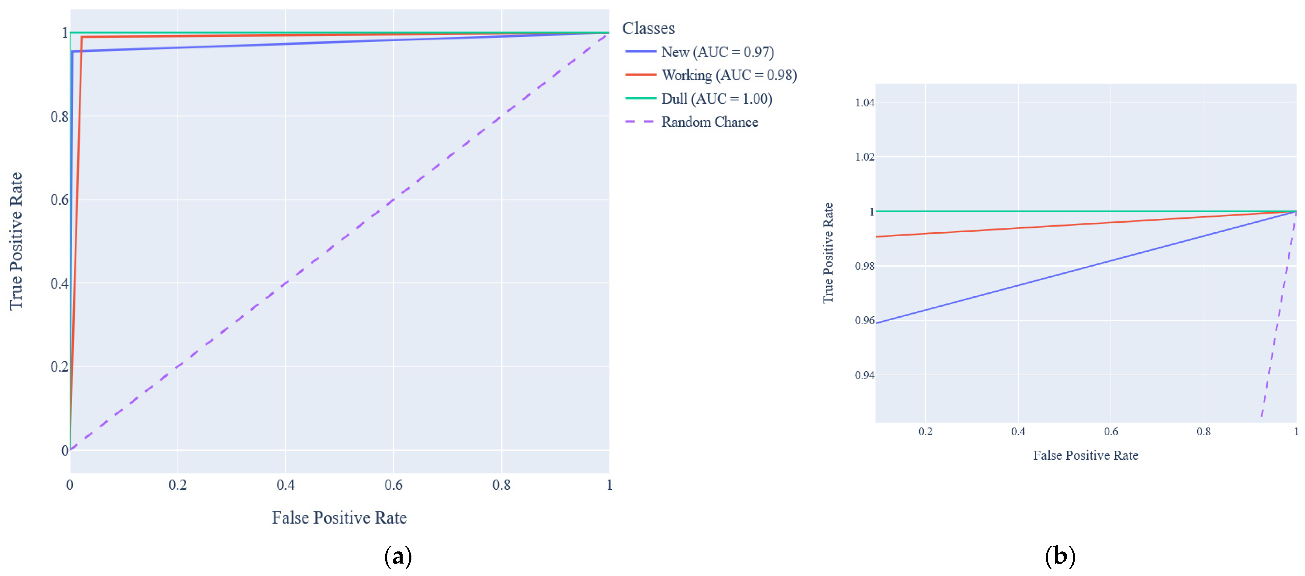
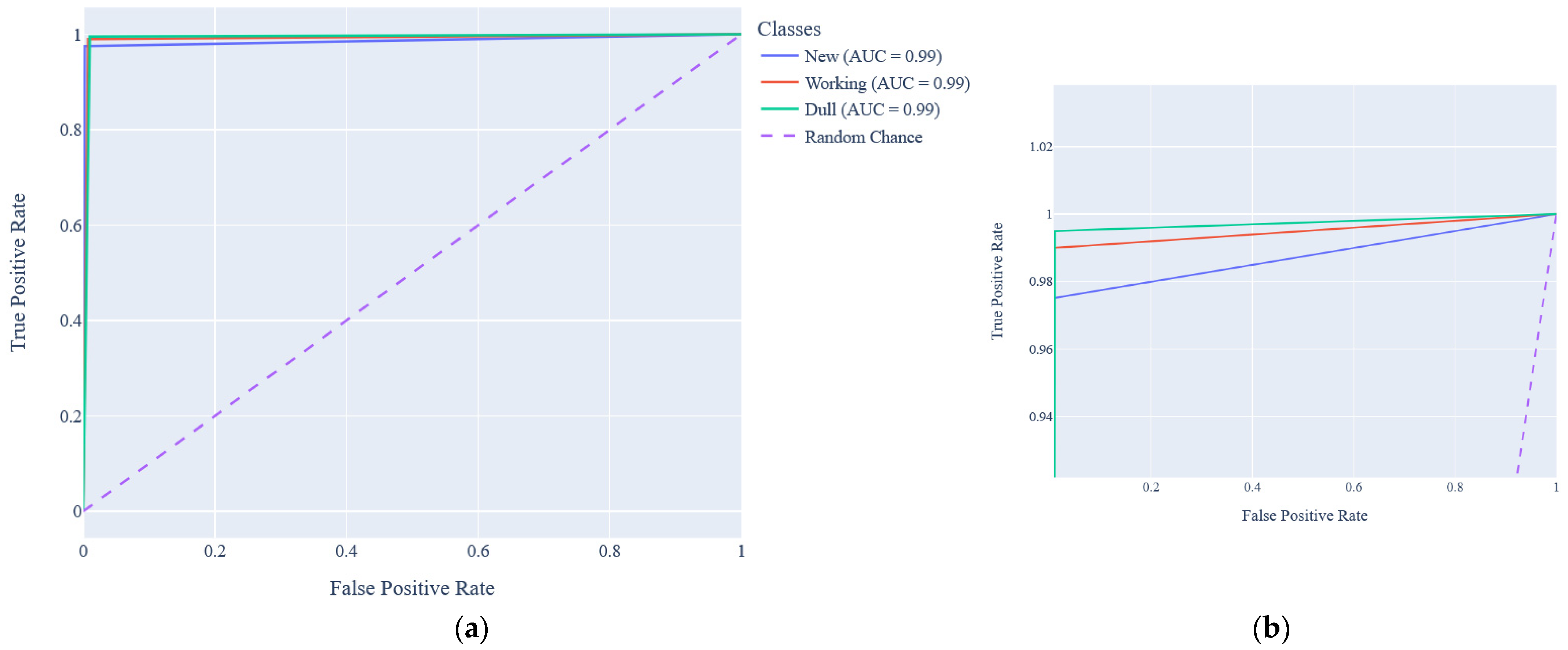
In summary, a prediction model was trained by utilizing the LSTM algorithm with the specified configuration parameters, including the dataset size, learning rate, number of epochs, and iterations per epoch. With an average accuracy of 94.85%, the LSTM algorithm effectively predicted outcomes based on the given dataset. The classification report and Receiver Operating Characteristics (ROC) curve are shown in Table 1 and Figure 12, respectively. From Figure 12, it was observed that the ROC curves for all three classes were closer to one, which indicates the accurate classification for all three classes. The classification accuracy of the model is 94.85%, indicating that the model correctly classifies 95% of all instances. The precision is 97.5%, meaning that when the model predicts positive, it is correct 97% of the time. The recall is 83%, showing that the model correctly identifies 83% of all actual positive cases. The F1 score, which balances precision and recall, is 94.66%. Finally, the specificity is 87.5%, indicating that 87.5% of the actual negative instances are correctly identified. High precision (94%) suggests the model is good at minimizing FPs. A high recall (94%) signifies that the model misses very few positive instances (false negatives). For monitoring tool wear over time, LSTMs can analyze sequences of sensor readings to predict future tool conditions based on historical patterns [46,47].

3.2.2. Feedforward Neural Network

The FFNN uses the Rectified Linear Unit (ReLu) activation function, which proposes non-linearity, enabling the network to capture complex relationships between input features and target labels. The final layer employs the softmax activation function to produce probabilistic predictions over multiple classes. The FFNN algorithm was trained using the same input data as the previous LSTM algorithm. Specific hyperparameters were set throughout the training to optimize the model’s performance. A learning rate of 0.001 was utilized, along with 100 epochs, a mini-batch size of 10, and 240 iterations per epoch. These hyperparameters were carefully chosen to enhance the training process and maximize the model’s accuracy.
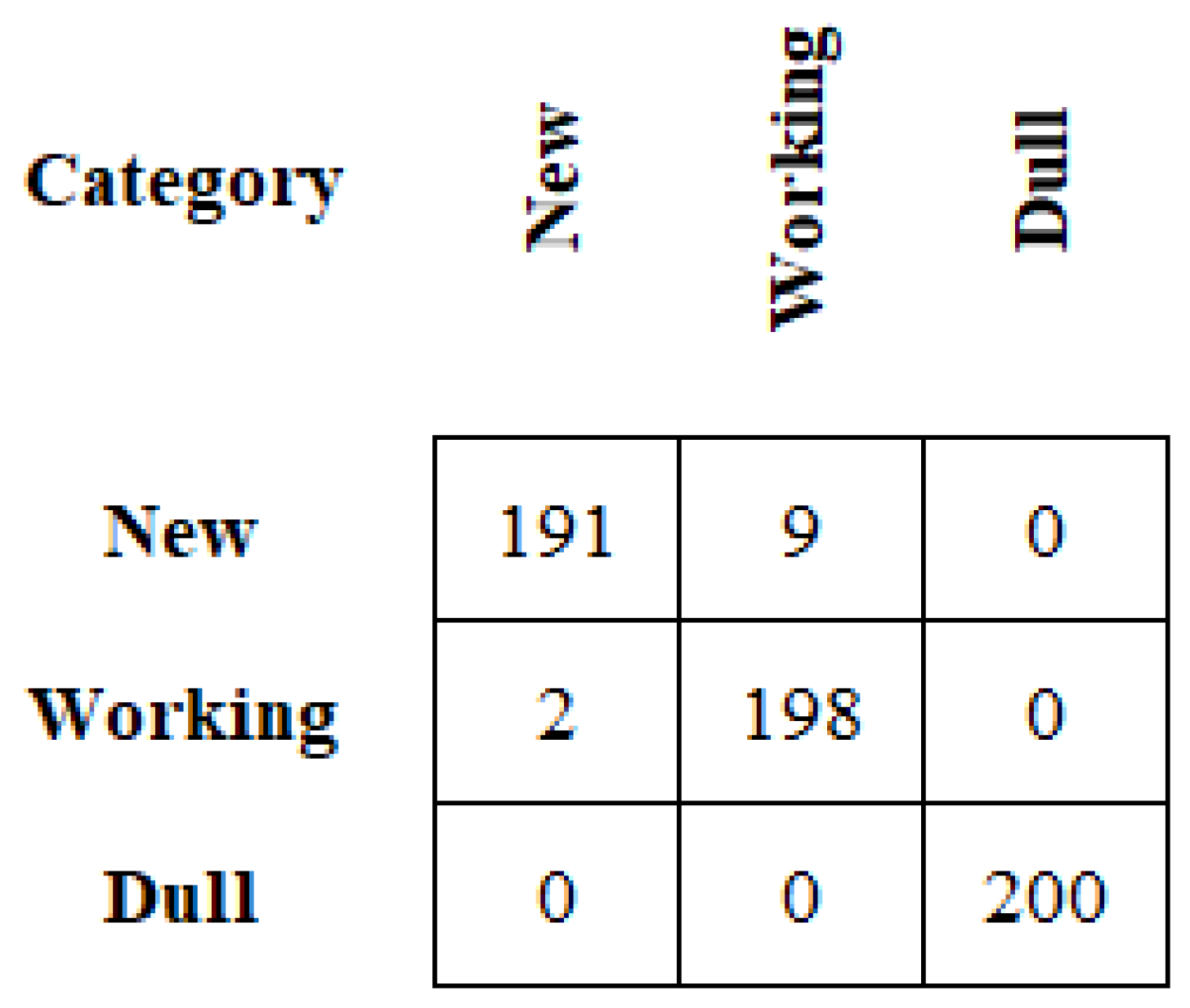
Figure 13 represents this confusion matrix, which visually depicts the performance of the model. The matrix consists of three rows and three columns. Examining the confusion matrix allows us to assess how effectively the model predicted different categories. It indicates that the model achieved a high accuracy rate in classifying the “dull” category, but it had a relatively higher tendency for misclassifications between the “new” and “working” categories. It has an overall classification accuracy of 98.16%. The kappa statistics value is also closer to 1 (0.9725). The ROC curve and classification report for FFNN are presented in Figure 14 and Table 2, respectively. An FFNN can model the intricate relationships between various sensor data and tool wear levels, improving the classification of tool conditions [48]. A similar result of DL was reported in the literature [49,50].

3.2.3. TCM Using RL Models

Q-Learning

The Q-learning algorithm was applied to the training data for several episodes, and it iteratively updated the Q-values based on monitored rewards and state transitions. Once the learning process was completed, the algorithm made predictions on the testing data. RL was successfully implemented in predictive maintenance problems [51]. The accuracy of the predictions was computed, and a confusion matrix was generated to analyze the model’s performance across different classes, depicted in Figure 15.
The results displayed in the confusion matrix indicate significant challenges in accurately classifying the instances. The model correctly predicted 192 samples as new, and 4 samples from this category were misclassified as working, while 4 samples were misclassified as “dull”. The model accurately identified 198 samples as working but misclassified 2 samples from this category as “new”. A total of 199 samples from the “dull” category were correctly classified as “dull”, while 1 sample was misclassified as a “working” tool. The average accuracy, calculated based on the values in the confusion matrix, was found to be 98.5%. This higher accuracy suggests that the reinforcement learning algorithms effectively capture the underlying patterns and features necessary for accurate classification. Considering the performance of the RL algorithms and the insights gained from the confusion matrix, it becomes evident that the employed algorithms were able to generalize well to the unseen dataset. The ROC curve and classification report for Q-learning are given in Figure 16 and Table 3, respectively. Q-learning operates based on a reward signal, which aligns well with TCM goals where the aim is to maximize positive outcomes [52].

3.2.4. SARSA

The SARSA algorithm was learned through multiple episodes by resetting the environment and selecting an initial state. Actions were chosen according to an epsilon-greedy policy, to balance the searching and operation. The algorithm updated the Q-values according to the observed rewards, and the learned Q-values were used to predict labels for the testing data. The results were visualized using a confusion matrix as shown in Figure 17. The average accuracy was 98.6%, indicating that the model correctly predicted the labels for the testing data. The ROC curve and classification report for SARSA are presented in Figure 18 and Table 4, respectively. It revealed that for TCM problems, RL algorithms can be successfully implemented. Thus, RL algorithms have been verified to be effective for TCM applications due to the balancing mechanism for exploration and exploitation [53]. The vibration signals with different ML algorithms yield different classification accuracies. SVM, KNN, and DT yielded classification accuracies of 90.8%, 81.3%, and 79.3%, respectively [54]. By tuning the KNN parameters, the authors yielded a classification accuracy of 93.7% [55]. Vibration signals with HE, yielded a classification accuracy of 99.98% [5]. In this work, the overall classification accuracies for LSTM, FFNN, Q-learning, and SARSA were 94.85%, 98.16%, 98.50%, and 98.66%, respectively. Compared with the literature, the results obtained from the present work are closer and the misclassification rate is very low. This indicates the effectiveness of the selected DL and RL models. Further, the model’s classification accuracy can be enhanced by tuning the hyperparameters.

3.3. Research Implications

Advancement in Predictive Maintenance: The DL and RL algorithms for TCM significantly enhance predictive maintenance strategies. High accuracy in the prediction of tool condition and failure enables prompt maintenance, decreasing downtime and increasing tool life. This may result in lower production costs, more effective manufacturing techniques, and higher-quality products. Industries can optimize their operations by switching from reactive to proactive maintenance.
Real-Time Monitoring and Decision Making: RL enables dynamic decision-making capabilities for TCMs. This dynamic approach can handle the variability in milling processes more effectively than static models. This adaptability can lead to increased productivity and the ability to handle customized production requirements.
Integration with Industry 4.0: By combining TCM with other Industry 4.0 technologies, like digital twins, cyber-physical systems, and the Industrial Internet of Things (IIoT), manufacturing environments can become more intelligent and networked. The development of “smart factories” where equipment can automatically check on itself, anticipate problems, and plan maintenance without human assistance may result from this integration.

4. Conclusions

In this work, during the milling of mild steel, TCMs were developed with DL (LSTM and FFNN) and RL (Q-learning and SARSA) algorithms using vibration signals. The following conclusions were arrived at from the research.
The tool wear has a substantial effect on vibration signals. When the tool loses its effectiveness at the cutting edge, it increases the tool-workpiece contact area and considerably increases the vibration amplitude.
DL algorithms such as LSTM and FFNN yielded a classification accuracy of 94.85% and 98.16%, respectively.
RL algorithms namely Q-learning and SARSA yielded a classification accuracy of 98.5% and 98.66% respectively.
The SARSA RL model performed better than other models in terms of classification accuracy, precision, recall, and F1 score.
The results obtained from the performance metrics indicated the superior performance of RL compared to DL due to the balancing mechanism for exploration and exploitation.
This balance is crucial in discovering effective tool conditions and avoiding premature convergence to suboptimal solutions.
The on-policy learning algorithm of SARSA through interaction with the environment ensures that the learning process is consistent with the actions being taken, which can be particularly useful in TCM applications.
RL algorithms have been recognized as an efficient model for TCM applications due to their learning behavior.

Author Contributions

Conceptualization, M.T. and P.P.; methodology, D.K.; software, S.G.; validation, M.T., P.P. and J.R.; formal analysis, A.P.; investigation, M.T.; resources, D.K.; data curation, D.K. and P.P.; writing—original draft preparation, M.T.; writing—review and editing, M.T. and A.P.; visualization, A.P.; supervision, M.T.; project administration, M.T. All authors have read and agreed to the published version of the manuscript.

Funding

This research received no external funding.

Data Availability Statement

The raw data supporting the conclusions of this article will be made available by the authors upon request.

Conflicts of Interest

The authors declare no conflicts of interest.

References

  1. Mohanraj, T.; Kirubakaran, E.S.; Madheswaran, D.K.; Naren, M.L.; Suganithi Dharshan, P.; Ibrahim, M. Review of advances in tool condition monitoring techniques in the milling process. Meas. Sci. Technol. 2024, 35, 092002. [Google Scholar]
  2. Mohanraj, T.; Shankar, S.; Rajasekar, R.; Sakthivel, N.; Pramanik, A. Tool condition monitoring techniques in milling process—A review. J. Mater. Res. Technol. 2020, 9, 1032–1042. [Google Scholar] [CrossRef]
  3. Kurada, S.; Bradley, C. A review of machine vision sensors for tool condition monitoring. Comput. Ind. 1997, 34, 55–72. [Google Scholar] [CrossRef]
  4. Wang, M.; Zhou, J.; Gao, J.; Li, Z.; Li, E. Milling tool wear prediction method based on deep learning under variable working conditions. IEEE Access 2020, 8, 140726–140735. [Google Scholar] [CrossRef]
  5. Mohanraj, T.; Yerchuru, J.; Krishnan, H.; Aravind, R.N.; Yameni, R. Development of tool condition monitoring system in end milling process using wavelet features and Hoelder’s exponent with machine learning algorithms. Measurement 2021, 173, 108671. [Google Scholar] [CrossRef]
  6. Chennai Viswanathan, P.; Venkatesh, S.N.; Dhanasekaran, S.; Mahanta, T.K.; Sugumaran, V.; Lakshmaiya, N.; Paramasivam, P.; Nanjagoundenpalayam Ramasamy, S. Deep learning for enhanced fault diagnosis of monoblock centrifugal pumps: Spectrogram-based analysis. Machines 2023, 11, 874. [Google Scholar] [CrossRef]
  7. Shankar, S.; Mohanraj, T.; Rajasekar, R. Prediction of cutting tool wear during milling process using artificial intelligence techniques. Int. J. Comput. Integr. Manuf. 2019, 32, 174–182. [Google Scholar] [CrossRef]
  8. Nair, V.S.; Rameshkumar, K.; Saravanamurugan, S. Chatter Identification in Milling of Titanium Alloy Using Machine Learning Approaches with Non-Linear Features of Cutting Force and Vibration Signatures. Int. J. Progn. Health Manag. 2024, 15. [Google Scholar] [CrossRef]
  9. Zhou, Y.; Sun, W. Tool wear condition monitoring in milling process based on current sensors. IEEE Access 2020, 8, 95491–95502. [Google Scholar] [CrossRef]
  10. He, Z.; Shi, T.; Xuan, J.; Li, T. Research on tool wear prediction based on temperature signals and deep learning. Wear 2021, 478, 203902. [Google Scholar] [CrossRef]
  11. Abdeltawab, A.; Xi, Z.; Longjia, Z. Enhanced tool condition monitoring using wavelet transform-based hybrid deep learning based on sensor signal and vision system. Int. J. Adv. Manuf. Technol. 2024, 132, 5111–5140. [Google Scholar] [CrossRef]
  12. Mannan, M.; Mian, Z.; Kassim, A.A. Tool wear monitoring using a fast Hough transform of images of machined surfaces. Mach. Vis. Appl. 2004, 15, 156–163. [Google Scholar] [CrossRef]
  13. De Barrena, T.F.; Ferrando, J.L.; García, A.; Badiola, X.; de Buruaga, M.S.; Vicente, J. Tool remaining useful life prediction using bidirectional recurrent neural networks (BRNN). Int. J. Adv. Manuf. Technol. 2023, 125, 4027–4045. [Google Scholar] [CrossRef]
  14. Natarajan, S.; Thangamuthu, M.; Gnanasekaran, S.; Rakkiyannan, J. Digital twin-driven tool condition monitoring for the milling process. Sensors 2023, 23, 5431. [Google Scholar] [CrossRef] [PubMed]
  15. Gupta, M.K.; Korkmaz, M.E.; Yılmaz, H.; Şirin, Ş.; Ross, N.S.; Jamil, M.; Królczyk, G.M.; Sharma, V.S. Real-time monitoring and measurement of energy characteristics in sustainable machining of titanium alloys. Measurement 2024, 224, 113937. [Google Scholar] [CrossRef]
  16. Arendra, A.; Herianto, H.; Akhmad, S.; Lumintu, I. Dimensions Reduction of Vibration Signal Features Using LDA and PCA for Real Time Tool Wear Detection with Single Layer Perceptron. In IOP Conference Series: Materials Science and Engineering; IOP Publishing: Bristol, UK, 2021. [Google Scholar]
  17. Gheisari, M.; Ebrahimzadeh, F.; Rahimi, M.; Moazzamigodarzi, M.; Liu, Y.; Dutta Pramanik, P.K.; Heravi, M.A.; Mehbodniya, A.; Ghaderzadeh, M.; Feylizadeh, M.R. Deep learning: Applications, architectures, models, tools, and frameworks: A comprehensive survey. CAAI Trans. Intell. Technol. 2023, 8, 581–606. [Google Scholar] [CrossRef]
  18. Hall, S.; Newman, S.T.; Loukaides, E.; Shokrani, A. ConvLSTM deep learning signal prediction for forecasting bending moment for tool condition monitoring. Procedia CIRP 2022, 107, 1071–1076. [Google Scholar] [CrossRef]
  19. Zhang, Q.; Xiao, J.; Tian, C.; Chun-Wei Lin, J.; Zhang, S. A robust deformed convolutional neural network (CNN) for image denoising. CAAI Trans. Intell. Technol. 2023, 8, 331–342. [Google Scholar] [CrossRef]
  20. Ross, N.S.; Shibi, C.S.; Mustafa, S.M.; Gupta, M.K.; Korkmaz, M.E.; Sharma, V.S.; Li, Z. Measuring Surface Characteristics in Sustainable Machining of Titanium Alloys Using Deep Learning-Based Image Processing. IEEE Sens. J. 2023, 23, 13629–13639. [Google Scholar] [CrossRef]
  21. Zhang, C.; Tan, K.C.; Li, H.; Hong, G.S. A cost-sensitive deep belief network for imbalanced classification. IEEE Trans. Neural Netw. Learn. Syst. 2018, 30, 109–122. [Google Scholar] [CrossRef]
  22. Dou, J.; Xu, C.; Jiao, S.; Li, B.; Zhang, J.; Xu, X. An unsupervised online monitoring method for tool wear using a sparse auto-encoder. Int. J. Adv. Manuf. Technol. 2020, 106, 2493–2507. [Google Scholar] [CrossRef]
  23. Cai, W.; Zhang, W.; Hu, X.; Liu, Y. A hybrid information model based on long short-term memory network for tool condition monitoring. J. Intell. Manuf. 2020, 31, 1497–1510. [Google Scholar] [CrossRef]
  24. Ou, J.; Li, H.; Huang, G.; Liu, B.; Wang, Z. Tool Wear Recognition Based on Deep Kernel Autoencoder with Multichannel Signals Fusion. IEEE Trans. Instrum. Meas. 2021, 70, 1–9. [Google Scholar] [CrossRef]
  25. Liao, D.; Shi, C.; Wang, L. A complementary integrated Transformer network for hyperspectral image classification. CAAI Trans. Intell. Technol. 2023, 8, 1288–1307. [Google Scholar] [CrossRef]
  26. Ross, N.S.; Sheeba, P.T.; Shibi, C.S.; Gupta, M.K.; Korkmaz, M.E.; Sharma, V.S. A novel approach of tool condition monitoring in sustainable machining of Ni alloy with transfer learning models. J. Intell. Manuf. 2024, 35, 757–775. [Google Scholar] [CrossRef]
  27. Liu, X.; Liu, S.; Li, X.; Zhang, B.; Yue, C.; Liang, S.Y. Intelligent tool wear monitoring based on parallel residual and stacked bidirectional long short-term memory network. J. Manuf. Syst. 2021, 60, 608–619. [Google Scholar] [CrossRef]
  28. Chen, M.; Li, M.; Zhao, L.; Liu, J. Tool wear monitoring based on the combination of machine vision and acoustic emission. Int. J. Adv. Manuf. Technol. 2023, 125, 3881–3897. [Google Scholar] [CrossRef]
  29. Cao, D.; Sun, H.; Zhang, J.; Mo, R. In-process tool condition monitoring based on convolution neural network. Comput. Integr. Manuf. Syst. 2020, 26, 74–80. [Google Scholar]
  30. Nguyen, V.; Nguyen, V.; Pham, V. Deep Stacked Auto-Encoder Network Based Tool Wear Monitoring in the Face Milling Process. J. Mech. Eng./Stroj. Vestn. 2020, 66. [Google Scholar] [CrossRef]
  31. Ma, J.; Luo, D.; Liao, X.; Zhang, Z.; Huang, Y.; Lu, J. Tool wear mechanism and prediction in milling TC18 titanium alloy using deep learning. Measurement 2021, 173, 108554. [Google Scholar] [CrossRef]
  32. Khandey, U.; Arya, V. Optimization of Multiple Surface Roughness Characteristics of Mild Steel Turned Product Using Weighted Principal Component and Taguchi Method. In Materials Today: Proceedings; Elsevier: Amsterdam, The Netherlands, 2023. [Google Scholar]
  33. Tran, Q.K.; Huynh, K.T.; Grall, A.; Langeron, Y.; Mosayebi Omshi, E. A Review on Reinforcement Learning in Condition-Based Maintenance; IDEALS: Champaign, IL, USA, 2023. [Google Scholar]
  34. Serin, G.; Sener, B.; Ozbayoglu, A.M.; Unver, H.O. Review of tool condition monitoring in machining and opportunities for deep learning. Int. J. Adv. Manuf. Technol. 2020, 109, 953–974. [Google Scholar] [CrossRef]
  35. Kaelbling, L.P.; Littman, M.L.; Moore, A.W. Reinforcement learning: A survey. J. Artif. Intell. Res. 1996, 4, 237–285. [Google Scholar] [CrossRef]
  36. Gnanasekaran, S.; Jakkamputi, L.P.; Rakkiyannan, J.; Thangamuthu, M.; Bhalerao, Y. A comprehensive approach for detecting brake pad defects using histogram and wavelet features with nested dichotomy family classifiers. Sensors 2023, 23, 9093. [Google Scholar] [CrossRef] [PubMed]
  37. Dimla, D.E. Sensor signals for tool-wear monitoring in metal cutting operations—A review of methods. Int. J. Mach. Tools Manuf. 2000, 40, 1073–1098. [Google Scholar] [CrossRef]
  38. Mehta, N.K.; Pandey, P.C.; Chakravarti, G. An investigation of tool wear and the vibration spectrum in milling. Wear 1983, 91, 219–234. [Google Scholar] [CrossRef]
  39. Chelladurai, H.; Jain, V.; Vyas, N. Development of a cutting tool condition monitoring system for high speed turning operation by vibration and strain analysis. Int. J. Adv. Manuf. Technol. 2008, 37, 471–485. [Google Scholar] [CrossRef]
  40. Dimla, D.E. The correlation of vibration signal features to cutting tool wear in a metal turning operation. Int. J. Adv. Manuf. Technol. 2002, 19, 705–713. [Google Scholar] [CrossRef]
  41. El-Wardany, T.; Gao, D.; Elbestawi, M. Tool condition monitoring in drilling using vibration signature analysis. Int. J. Mach. Tools Manuf. 1996, 36, 687–711. [Google Scholar] [CrossRef]
  42. Orhan, S.; Er, A.O.; Camuşcu, N.; Aslan, E. Tool wear evaluation by vibration analysis during end milling of AISI D3 cold work tool steel with 35 HRC hardness. NDT E Int. 2007, 40, 121–126. [Google Scholar] [CrossRef]
  43. Dimla, D.; Lister, P. On-line metal cutting tool condition monitoring.: I: Force and vibration analyses. Int. J. Mach. Tools Manuf. 2000, 40, 739–768. [Google Scholar] [CrossRef]
  44. Ma, K.; Wang, G.; Yang, K.; Hu, M.; Li, J. Tool wear monitoring for cavity milling based on vibration singularity analysis and stacked LSTM. Int. J. Adv. Manuf. Technol. 2022, 120, 4023–4039. [Google Scholar] [CrossRef]
  45. Zheng, G.; Sun, W.; Zhang, H.; Zhou, Y.; Gao, C. Tool wear condition monitoring in milling process based on data fusion enhanced long short-term memory network under different cutting conditions. Eksploat. I Niezawodn. 2021, 23, 612–618. [Google Scholar] [CrossRef]
  46. Chan, Y.-W.; Kang, T.-C.; Yang, C.-T.; Chang, C.-H.; Huang, S.-M.; Tsai, Y.-T. Tool wear prediction using convolutional bidirectional LSTM networks. J. Supercomput. 2022, 78, 810–832. [Google Scholar] [CrossRef]
  47. Chen, Q.; Xie, Q.; Yuan, Q.; Huang, H.; Li, Y. Research on a real-time monitoring method for the wear state of a tool based on a convolutional bidirectional LSTM model. Symmetry 2019, 11, 1233. [Google Scholar] [CrossRef]
  48. Chen, Y.; Jin, Y.; Jiri, G. Predicting tool wear with multi-sensor data using deep belief networks. Int. J. Adv. Manuf. Technol. 2018, 99, 1917–1926. [Google Scholar] [CrossRef]
  49. Patil, S.S.; Pardeshi, S.S.; Pradhan, N.; Patange, A.D. Cutting tool condition monitoring using a deep learning-based artificial neural network. Int. J. Perform. Eng. 2022, 18, 37. [Google Scholar]
  50. Ou, J.; Li, H.; Huang, G.; Zhou, Q. A Novel Order Analysis and Stacked Sparse Auto-Encoder Feature Learning Method for Milling Tool Wear Condition Monitoring. Sensors 2020, 20, 2878. [Google Scholar] [CrossRef] [PubMed]
  51. Siraskar, R.; Kumar, S.; Patil, S.; Bongale, A.; Kotecha, K. Reinforcement learning for predictive maintenance: A systematic technical review. Artif. Intell. Rev. 2023, 56, 12885–12947. [Google Scholar] [CrossRef]
  52. Ding, Y.; Ma, L.; Ma, J.; Suo, M.; Tao, L.; Cheng, Y.; Lu, C. Intelligent fault diagnosis for rotating machinery using deep Q-network based health state classification: A deep reinforcement learning approach. Adv. Eng. Inform. 2019, 42, 100977. [Google Scholar] [CrossRef]
  53. Marugán, A.P. Applications of Reinforcement Learning for maintenance of engineering systems: A review. Adv. Eng. Softw. 2023, 183, 103487. [Google Scholar] [CrossRef]
  54. Zhou, C.A.; Yang, B.; Guo, K.; Liu, J.; Sun, J.; Song, G.; Zhu, S.; Sun, C.; Jiang, Z. Vibration singularity analysis for milling tool condition monitoring. Int. J. Mech. Sci. 2020, 166, 105254. [Google Scholar] [CrossRef]
  55. Zhou, C.; Jiang, X.; Sun, C.; Zhu, Z. The Monitoring of Milling Tool Tipping by Estimating Holder Exponents of Vibration. IEEE Access 2020, 8, 96661–96668. [Google Scholar] [CrossRef]
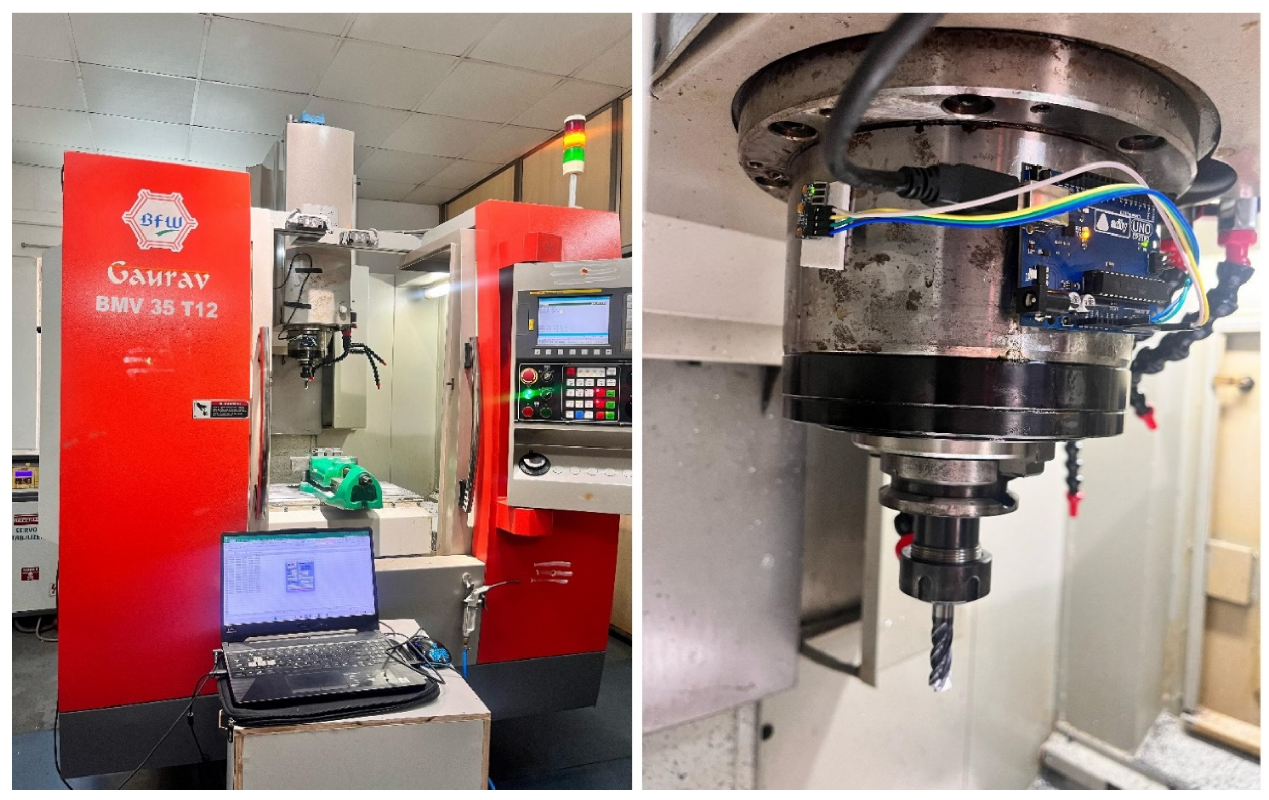
Figure 1. Experimental setup.
Jsan 13 00042 g001
Figure 2. Representation of the DL model.
Jsan 13 00042 g002
Figure 3. LSTM of architecture.
Jsan 13 00042 g003
Figure 4. Architecture of FFNN.
Jsan 13 00042 g004
Figure 5. Block diagram of RL.
Jsan 13 00042 g005
Figure 6. Representation of Q-learning.
Jsan 13 00042 g006
Figure 7. Resultant vibration signal for various tools.
Jsan 13 00042 g007
Figure 8. RMS of Resultant vibration for various tools.
Jsan 13 00042 g008
Figure 9. Kurtosis of Resultant vibration for various tools.
Jsan 13 00042 g009
Figure 10. Skewness of Resultant vibration for various tools.
Jsan 13 00042 g010
Figure 11. Confusion matrix for the LSTM algorithm.
Jsan 13 00042 g011
Figure 12. (a) ROC curve for LSTM (b) enlargement of overlapping part.
Jsan 13 00042 g012
Figure 13. Confusion matrix of FFNN algorithm.
Jsan 13 00042 g013
Figure 14. (a) ROC curve for FFNN, (b) enlargement of overlapping part.
Jsan 13 00042 g014
Figure 15. Confusion matrix generated by Q-learning algorithm.
Jsan 13 00042 g015
Figure 16. (a) ROC curve for Q-learning, (b) enlargement of overlapping part.
Jsan 13 00042 g016
Figure 17. Confusion matrix obtained from the SARSA algorithm.
Jsan 13 00042 g017
Figure 18. (a) ROC curve for SARSA, (b) enlargement of overlapping part.
Jsan 13 00042 g018
Table 1. Classification Report—LSTM.
Classes/MetricsPrecisionRecallFPRF1 ScoreSupport
New0.93781.00000.03001.0000200
Working0.90820.90500.04750.9211200
Dull1.00000.94000.00000.9238200
Overall accuracy: 0.9485; Kappa statistics: 0.9225
Table 2. Classification Report—FFNN.
Classes/MetricsPrecisionRecallFPRF1 ScoreSupport
New0.95960.95500.00500.9720200
Working0.98650.99000.02250.9729200
Dull1.00001.00000.00001.0000200
Overall accuracy: 0.9816; Kappa statistics: 0.9725
Table 3. Classification Report—Q-learning.
Classes/MetricsPrecisionRecallFPRF1 ScoreSupport
New0.98510.99500.00500.9900200
Working0.98970.97000.01250.9797200
Dull0.98010.99000.00750.9850200
Overall accuracy: 0.9850; Kappa statistics: 0.9775
Table 4. Classification Report—SARSA.
Classes/MetricsPrecisionRecallFPRF1 ScoreSupport
New0.97050.99500.00250.9875200
Working0.98500.97500.00750.9848200
Dull0.98010.99000.01000.9875200
Overall accuracy: 0.9866; Kappa statistics: 0.9800
Disclaimer/Publisher’s Note: The statements, opinions and data contained in all publications are solely those of the individual author(s) and contributor(s) and not of MDPI and/or the editor(s). MDPI and/or the editor(s) disclaim responsibility for any injury to people or property resulting from any ideas, methods, instructions or products referred to in the content.