Network Attack Classification in IoT Using Support Vector Machines ^†

Abstract

Machine learning (ML) techniques learn a system by observing it. Events and occurrences in the network define what is expected of the network’s operation. It is for this reason that ML techniques are used in the computer network security field to detect unauthorized intervention. In the event of suspicious activity, the result of the ML analysis deviates from the definition of expected normal network activity and the suspicious activity becomes apparent. Support vector machines (SVM) are ML techniques that have been used to profile normal network activity and classify it as normal or abnormal. They are trained to configure an optimal hyperplane that classifies unknown input vectors’ values based on their positioning on the plane. We propose to use SVM models to detect malicious behavior within low-power, low-rate and short range networks, such as those used in the Internet of Things (IoT). We evaluated two SVM approaches, the C-SVM and the OC-SVM, where the former requires two classes of vector values (one for the normal and one for the abnormal activity) and the latter observes only normal behavior activity. Both approaches were used as part of an intrusion detection system (IDS) that monitors and detects abnormal activity within the smart node device. Actual network traffic with specific network-layer attacks implemented by us was used to create and evaluate the SVM detection models. It is shown that the C-SVM achieves up to 100% classification accuracy when evaluated with unknown data taken from the same network topology it was trained with and 81% accuracy when operating in an unknown topology. The OC-SVM that is created using benign activity achieves at most 58% accuracy.

1. Introduction

The Internet of Things (IoT) is increasingly becoming a bigger part of our everyday routine. Smart heterogeneous IoT devices are now connected to each other, forming their own network that can be accessed remotely. IoT applications include smart cities, intelligent transportation, responsive environments, and many more, which rely on timely and reliable data to achieve their full potential. Lack of, or compromised data, due to device failure or malicious intrusion within the IoT, may result in unfortunate and unforeseen outcomes. Early detection of misbehavior and early response to the intrusion or device failure can preserve and maintain the application’s goal.

Establishing a secure and reliable network partially depends on preventing and anticipating possible threats. Threats can be environmental, physical, but also intentional. Environmental and physical threats can be prevented, to some extend, by ensuring that proper infrastructure security is applied. Malicious disruptions of the IoT network data flow may also be prevented for some of the known threats. The device connecting the IoT network to the Internet (called the Gateway or Sink node) can prevent malicious threats from acting on the network based on a predefined set of rules that allow or disallow communications. The set of rules is usually applied through the use of a firewall. Nevertheless, there exist new threats and/or variations of old threats, which cannot be anticipated and can penetrate the prevention security measures and attack the network.

Detection of intrusions at an early stage can prevent attacks from causing irreversible damage. There are two major detection methods in intrusion detection systems (IDS): the pattern detection-based mechanism and anomaly detection-based mechanism [1]. The former relies on knowledge of existing attacks and their patterns; whereas the latter can capture never before seen attacks by identifying abnormalities within the network.

Despite the maturity of IDS technology for traditional networks, current solutions are inadequate for wireless sensor network (WSN) and IoT systems, because of IDS computational and memory requirements. The processing and storage capacity of network nodes that host IDS agents is an important issue. In traditional networks, the IDS agents are deployed in high computational and memory capacity devices. The IoT networks are usually composed of nodes with resource constraints in which finding nodes with the ability to support IDS agents is harder. Furthermore, the IoT network architecture plays a decisive role in the selection of security measures to be employed. In traditional networks, end systems are directly connected to specific nodes (e.g., wireless access points, switches, and routers) that are responsible for forwarding the packets to the destination. WSN and IoT networks, on the other hand, are usually formed in wireless mesh topologies, using multi-hop communication to reach the gateways and/or the destination.

The WSN and IoT use network protocols to establish multi-hop communication that are not employed in traditional networks, bringing new security challenges. Network routing protocols such as IPv6 over Low-power Wireless Personal Area Network (6LoWPAN), IEEE 802.15.4, and Pv6 Routing Protocol for Low-Power and Lossy Networks (RPL) are some of the protocols that are being used. The selection of routing protocol relies on, among others, the IoT application and device specifications making each IoT network specific enough to the application and less compliant to the standard security measures.

The current work evaluates supervised learning techniques as anomaly detection techniques using actual network traffic and concludes that using activity from a compromised setting has better results. The main anomaly profiling techniques can be categorized as applying thresholds, game theory, fuzzy logic, machine learning, and biologically inspired techniques. Two support vector machine (SVM) models are evaluated to be used as IDS agents: the classification SVM (C-SVM) and the one-class SVM (OC-SVM). The two SVM classification techniques were used to emphasize the importance of using abnormal activity when creating detection models. Previous work on SVM evaluated the accuracy results of the C-SVM detection models when trained and evaluated in the same network topology. The accuracy metric alone offers partial information on classification efficacy [2,3]. In this work, the results are presented using multiple binary classification metrics and explore precision and sensitivity, along with accuracy and the quality of the binary classification of two SVM classification techniques and in two network topologies. The SVM detection models were created using local node network packet activity. The OC-SVM is created with local node activity when executing the intended application with no malicious intervention; the benign application. For creating the C-SVM detection model, node activity was used from the benign application and activity when the node is compromised; the malicious application. The SVM models were evaluated in an unfamiliar network topology against three types of attacks (and their variations). A general routing layer was used to implement the attacks, so that to eliminate artifacts stemming from control messages of more complex protocols, like Routing Protocol for Low Power and Lossy Networks (RPL) over 6LowPAN (Low power Wireless Personal Area Networks [4]. C-SVM, when evaluated with unknown activity, achieved up to 100% classification accuracy, approximately 49% more than OC-SVM, in which the highest accuracy achieved was 60.8%. The results corroborate with the findings of previous work [1], that using both benign and malicious activity provides better understanding of the node status and better detection rates.

In summary, the contributions of this paper are as follows: (i) use of actual network traffic, (ii) use of supervised learning for network-layer attack classification in WSN and IoT networks, (iii) use of two SVM techniques, namely classification and one-class, (iv) evaluation and contrast of the two SVM techniques on two topologies and five attacks, (v) combination of data and models to provide a generalized detection for all attacks, (vi) establishment of the suitability of C-SVM in detecting the attacks in unknown topologies and (vii) verification of the superiority of C-SVM vs. OC-SVM in detecting network-layer attacks in WSN and IoT Networks.

The rest of the paper is structured as follows: Section 2 presents background information on SVM. Section 3 presents the methodology used to create IDS using SVM and Section 4 presents the training and evaluations results of the proposed solutions. Section 5 discusses related work on machine learning detection techniques and IDS. Section 6 concludes the current work.

2. Background

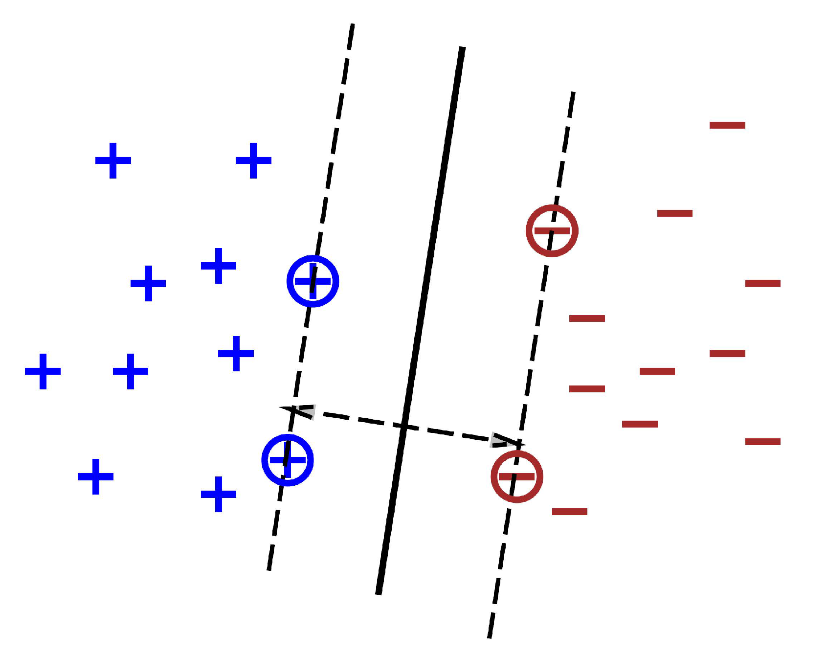
Support vector machines (SVM) are a class of supervised machine learning algorithms that create a binary classification model out of complex highly non-linear problems [5]. The SVM requires data samples to create a hyperplane, the decision surface, and maximize the margin around it (see Figure 1). It undergoes a training phase in which each data sample, denoted as $x_i$, is assigned to the class it belongs to, denoted as $y_i$, the predicted value. Therefore, the training set is labeled in pairs $(x_i,y_i),i=1,\cdots ,l$ where $x\in {\mathbb{R}}^n$ and $y\in \{1,-1\}$. The data sample includes the so called features, which are the data parameters that are used to define the activity of the data sample vector. The end result of the SVM training phase is a set of support vectors that create the optimal hyperplane and the weights $w_i$, which correspond to each input feature that is used to predict the value of y. The difference of the SVM from other neural networks is that it uses the optimization of maximizing the margin to reduce the number of weights that are nonzero to just a few. These correspond only to the important features that provide useful information in deciding the hyperplane.

One important step in the SVM is the kernel function that helps change the data dimensions and in turn determine the shape of the hyperplane. In simple words, the kernel function adds dimensions in the hyperplane so that a clear distinction between the classes can be made. There are various types of kernels available to use, which include the Linear, Polynomial, Gaussian Radial Basis Function (RBF) and Sigmoid. The results of each kernel depend on the nature of the data sample. The Linear kernel is the simplest kernel that has better results when used in linear problems. The polynomial, RBF and Sigmoid kernels attempt to generate support vectors from a combination of the features given. They are best used with non-linear data, but their complexity relies on the number of new features they extract.

3. Methodology for IDS Using SVM

The following section presents the steps taken to create and evaluate the C-SVM and OC-SVM detection machines. It describes the C-SVM and OC-SVM models, the kernel used to create the hyperlane, the scaling performed on the input data and how the free parameters are computed.

3.1. C-Support Vector Machine

The C-support optimization type of SVM is used when there is more than one class of data. In our case, we have two classes: benign and malicious. Consider the training set $x_i\in {\mathbb{R}}^n$, where $i=1,\cdots ,l$; $x_i$ is separated in two classes; $y\in {\mathbb{R}}^l$ such that $y_i\in \{1,-1\}$; l is the number of local node activity. C-SVM solves the optimization problem shown in Equation (1) [7].

$$\begin{array}{c}\hfill \underset{\mathbf{\omega },b,\mathbf{\xi }}{min}\\ \hfill \mathrm{subject} \mathrm{to}\\ \hfill \end{array}\begin{array}{cc}\hfill & {\displaystyle \frac{1}{2}{\mathbf{\omega }}^{⊺}\mathbf{\omega }+C\sum _{i=1}^l{\xi }_i}\hfill \\ \hfill & y_i({\mathbf{\omega }}^{⊺}\mathbf{\varphi }\left({\mathit{x}}_{\mathit{i}}\right)+b)\ge 1-{\xi }_i\hfill \\ \hfill & {\xi }_i\ge 0,i=1,\cdots ,l\hfill \end{array}$$

(1)

In Equation (1), $\varphi \left(x_i\right)$ maps $x_i$ into a higher-dimensional space and $C>0$ is the regularization parameter. Due to the possible high dimensionality of the weights w, we solve the problem shown in Equation (2) [7].

$$\begin{array}{c}\hfill \underset{\mathbf{\alpha }}{min}\\ \hfill \mathrm{subject} \mathrm{to}\\ \hfill \end{array}\begin{array}{cc}\hfill & \frac{1}{2}{\mathbf{\alpha }}^{⊺}Q\mathbf{\alpha }-{\mathit{e}}^{⊺}\mathbf{\alpha }\hfill \\ \hfill & {\mathit{y}}^{⊺}\mathbf{\alpha }=0\hfill \\ \hfill & 0\le {\mathbf{\alpha }}_i\le C,i=1,\cdots ,l\hfill \end{array}$$

(2)

In Equation (2), $e={[1,\cdots ,1]}^{⊺}$ is the vector of all ones, Q is an l by l positive semi-definite matrix, $Q_{i,j}\equiv y_i{y}_{j}K({\mathit{x}}_{\mathit{i}},{\mathit{x}}_{\mathit{j}})$ is the kernel function. The kernel function we used for our purposes is discussed in Section 3.4. After we solve Equation (2), we solve Equation (3) to find the optimal w.

$${\displaystyle \mathbf{\omega }=\sum _{i=1}^l{y}_i{\alpha }_i\varphi \left({\mathit{x}}_{\mathit{i}}\right)}$$

(3)

The decision function for the C-class SVM is shown in Equation (4) [7].

$$sgn({\mathbf{\omega }}^{⊺}\varphi \left(\mathit{x}\right)+b)=sgn\left(\sum _{i=1}^l{y}_i{\alpha }_{i}K({\mathit{x}}_{\mathit{i}},\mathit{x})+b\right)$$

(4)

3.2. OC-Support Vector Machine

One class SVMs are trained on what is defined as normal activity profile [5]. The model is trained only by normal activity and any deviation from what is considered normal raises an alarm. Assuming that the training set of the one class SVM is $x_i\in {\mathbb{R}}^n$, where $i=1,\cdots ,l$; and $y\in {\mathbb{R}}^l$ such that $y_i\in \{1,-1\}$; l is the number of local node activity. The values of $x_i$ are taken from the benign local sensor activity. Label $y_i$ was also used at the training stage and labeled as benign class. To create the detection models, we solve the following equation [7,8]:

$$\begin{array}{c}\hfill \underset{\mathbf{\omega },\mathbf{\xi },\mathbf{\rho }}{min}\\ \hfill \mathrm{subject} \mathrm{to}\\ \hfill \end{array}\begin{array}{cc}\hfill & {\displaystyle \frac{1}{2}{\mathbf{\omega }}^{⊺}\mathbf{\omega }-\rho +\frac{1}{\nu l}\sum _{i=1}^l{\xi }_i}\hfill \\ \hfill & {\mathbf{\omega }}^{⊺}\varphi \left({\mathit{x}}_{\mathit{i}}\right)\ge \rho -{\xi }_i\hfill \\ \hfill & {\xi }_i\ge 0,i=1,\cdots ,l\hfill \end{array}$$

(5)

To find the dual problem as in [7], we solve:

$$\begin{array}{c}\hfill \underset{\mathbf{\alpha }}{min}\\ \hfill \mathrm{subject} \mathrm{to}\\ \hfill \end{array}\begin{array}{cc}\hfill & \frac{1}{2}{\mathbf{\alpha }}^{⊺}Q\mathbf{\alpha }\hfill \\ \hfill & 0\le {\mathbf{\alpha }}_i\le \frac{1}{\nu l},i=1,\cdots ,l,\hfill \\ \hfill & {\mathit{e}}^{⊺}\mathbf{\alpha }=1,\hfill \end{array}$$

(6)

where $Q_{ij}=K(x_i,x_j)=\varphi {\left(x_i\right)}^{⊺}\varphi \left(x_j\right)$. The end decision function is as follows:

$$sgn\left(\sum _{i=1}^l{\mathbf{\alpha }}_{i}K({\mathit{x}}_{\mathit{i}},\mathit{x})-\rho \right)$$

(7)

3.3. Scaling

Scaling is applied to both training and evaluation data sets to construct the data in a form that the SVM can take as input and construct the hyperplane. Scaling is also used to eliminate possible cases in which certain features that are in greater numeric ranges dominate those in smaller numeric ranges [7]. At the same time, applying scaling returns the parameters that are the most important to retrieve better results [7,9].

We apply scaling for all support vectors $(x_i,y_i)$ using the following:

$${\mathit{x}}_{\mathit{i}}^{\prime }=(\beta -\alpha ){\displaystyle \frac{x_i-minx}{maxx-minx}}+a$$

(8)

where ${\mathit{x}}_{\mathit{i}}^{\prime }$ is the scaling of parameter $i>0$ and $x>0$. Furthermore, $minx$ and $maxx$ is the minimum and maximum numbers of the input vector. The constants $[\alpha ,\beta ]$ correspond to the scaling range in our case $[-1,1]$. The scaling does not change the labels $y_i$.

Scaling our data returns the support vectors with the significant parameters that are later used as inputs to our SVM. Parameters that were scaled to 0 are not included, as they do not provide any useful information to our SVM model.

3.4. Radial Basis Function Kernel

For the current work, we chose the RBF (Gaussian) kernel, as it had better results compared to other kernels (see Equation (9)). The RBF was compared against the linear, polynomial and the sigmoid kernel. The RBF identified the support vectors required to classify correctly unknown data with less computational complexity [4].

$$\begin{array}{cc}\hfill & K({\mathit{x}}_{\mathit{i}},{\mathit{x}}_{\mathit{j}})=exp(-\gamma \Vert {\mathit{x}}_{\mathit{i}}-{\mathit{x}}_{\mathit{j}}{\Vert }^2),\hfill \\ \hfill & \gamma >0,\gamma =\frac{1}{2{\sigma }^2}\hfill \\ \hfill & \sigma \mathrm{is} \mathrm{a} \mathrm{free} \mathrm{parameter}\hfill \end{array}$$

(9)

3.5. Cross-Validation and Grid Search

The SVM and RBF kernel use the free parameters C and $\gamma$ for the Equations (2) and (9). The parameters $(C,\gamma )$ are used to maximize the margin of the SVM hyperplane. It is an important step to avoid over-fitting the data. SVM aims in maximizing the margin from the hyperplane to avoid misclassification errors [7]. The parameters are chosen through the cross-validation and grid search methods that extensively evaluate the $(C,\gamma )$ values against the input data set. The cross validation technique splits the data to training and evaluation. The grid search evaluates pairs of $(C,\gamma )$ against the input data to find the best pair for the best hyperplane margin.

4. SVM Models Training and Evaluation

There are two stages of SVM, the training stage and the evaluation stage. At the training stage, the SVM takes as input training data and creates a hyperplane. The classification hyperplane, the detection model, is evaluated using data that were not used at the training stage. The SVM model maps the data into the hyperplane and returns the classification result y. The data used in both stages were retrieved from two set of scenarios and two different network topologies.

Figure 2a,b shows the two types of network topologies that have been used for the current work. Each figure shows the Sink node to be either in the middle of the network or on a corner of the network and the hop distance of each node to the Sink (shown in the node). Figure 2a, places the Sink in the middle and is considered to be the best case scenario as four nodes are one hop away from the Sink and the maximum distance from the Sink is only four hops. The sensor activity used for training the SVM models were taken from experimental results from the Sink-in-the-Middle topology. SVM models were also created as a general approach to detect the presence of any attack within the network. The same general SVM model, trained for the Sink in the middle topology, was also evaluated against a new topology where the Sink is placed at the top left corner of the network (see Figure 2b. The network topology in which the Sink is found on top of the network has only two nodes directly connected to the Sink, and the farthest node is eight hops away.

To create the dataset for two class activities, the benign and the malicious, two types of experimental scenarios were used. The benign scenarios, in which all nodes within the network were executing the benign intended application, and the malicious scenarios, in which at least one node, except the Sink node, was malicious. From each node, a set of parameters was collected and used in the creation and evaluation of its IDS model (shown in

Table 1. Routing layer parameters used as input in the SVM models.

Local Node Monitoring Parameters
Data Packets Received	Data Packets Sent
Packets Forwarded	Packets Dropped
Announcements Received

). The parameters are taken from the routing layer, the layer the attacks exploit. Prior work has shown that when using parameters from the layer under attack, the IDS achieves better results compared to when using parameters from other layers [3,10,11,12]. Specifically, 80% randomly selected data values from both classes were used for the training stage and the other 20% were used to evaluate the detection models.

For the current work, we used the attacks from the work of [1] and the RMT tool to collect the data [10]. There are three major routing layer category attacks, the Selective Forward (SF), Blackhole (BH), and Sinkhole. The SF attacks drop packets randomly either by using a predefined ratio (Forwarding Ratio (FR)) or by selectively choosing which neighbor’s packets to drop (Block Node (BN)). For the current work, the ratio of the FR attack was set to 50%. Each packet received by the malicious node has a 50% probability to be forwarded or dropped. The probability ratio is determined by a random function. The BN version of the attack randomly chooses a neighbor to not forward its packets. The choice of the neighbor to block changes throughout the experiment. In our case, a new target node is selected every time the malicious node receives 10 packets from its current target. The Blackhole attack complements the SF attacks to create a greater effect. BH attack lures the traffic towards the malicious node, advertising that is one hop away from the Sink node and in turn the SF selectively chooses which packet to forward. The Sinkhole attack advertises that the malicious node is the Sink, aiming to gather the traffic and never allow them to reach their destination.

The data was collected from each node at predefined time intervals called epochs and averaged per the distance of the sensor nodes from the Sink node [10]. Each epoch was set to one (1) minute and the total number of epochs used per distance was 25. The benign application is a periodic one, and each sensor generated 60 packets per minute for an effective data rate of 384 bps.

Each epoch represents local node activity for a specific hop distance from the Sink. Therefore, the number of epochs from each simulation used for the training and evaluation depends on the number of hops from the Sink. The exact number of epochs used for the training set and the evaluation set are shown in

Table 2. SVM training data set when Sink is in the middle.

Attack		C-SVM			OC-SVM
		Benign	Viral	Total	Benign	Viral	Total
SF 1	BN 2	80	80	160	80	0	80
	FR 3	80	80	160	80	0	80
SF & BH 4	BN	80	80	160	80	0	80
	FR	80	80	160	80	0	80
Sinkhole		80	80	160	80	0	80
Sink in the middle (All attacks)		80	400	480	80	0	80

¹ SF = Selective Forward. ² BN = Block Node. ³ FR = Forwarding Ratio. ⁴ BH = Blackhole.

and

Table 3. SVM evaluation data set when Sink is in the middle.

Attack		C-SVM			OC-SVM
		Benign	Viral	Total	Benign	Viral	Total
SF	BN	20	20	40	20	100	120
	FR	20	20	40	20	100	120
SF & BH	BN	20	20	40	20	100	120
	FR	20	20	40	20	100	120
Sinkhole		20	20	40	20	100	120
Sink in the middle (All attacks)		20	100	120	20	500	520
Sink on Top (All attacks)		200	800	1000	200	800	1000

. Table 2 shows that no data was used for training any SVM model in the setting of the network topology where the Sink was on top of the network (see Figure 2b). The number of epochs for the Sink-on-Top is higher than when the sink was in the middle since the number of hops is eight instead of four, and all data gathered from the Sink-on-Top experiments were only used in the evaluation stage.

4.1. Training of the SVM Models

In our case, we have two classes, the benign and the viral class, denoted $-1$ and 1, respectively.

To construct the training model, we use the following steps [13]:

• Label data into either benign and malicious class in the form of vectors $(x_i,y_i)$.
• Apply scaling to the training set.
• Apply RBF kernel to the training set.
• Apply cross validation.
• Conduct a grid search to the training set to retrieve the best values of $(C,\gamma )$.
• Input the training set and $(C,\gamma )$ values, when training for C-SVM, to create the SVM model.

Steps 1 to 3 were applied for both SVM models. Steps 4 and 5 were only used to retrieve values C and $\gamma$ of the C-SVM detection model. The last step was to use as input the training data to the SVM training and get the SVM model. For the OC-SVM, the training was conducted only on the benign data and as a result only one detection model was created and evaluated against the routing attacks. On the contrary, for the C-SVM method, one detection model was created for each routing attack.

For the C-SVM method, the significant parameters for each detection model varied based on the attack. For Selective Forward attacks, the scaling step returns data for the parameters data packets received ($P_{RC}$), packets forwarded ($P_{FR}$), number of packets dropped ($P_{DR}$) and the number of announcements received ($P_{An}$). For the Sinkhole attack, the scaling step returns the training set for all five parameters shown in

Table 4. SVM evaluation data set when Sink is in the middle.

Monitored Routing Layer Parameters	C-SVM					OC-SVM
	SF		SF & BH		Sinkhole
	FR	BN	FR	BN
Data Packets Received ($P_{RC}$)	✔	✔	✔	✔	✔	✔
Data Packets Sent ($P_{St}$)					✔
Packets Forwarded ($P_{FR}$)	✔	✔	✔	✔	✔	✔
Packets Dropped ($P_{DR}$)	✔	✔	✔	✔	✔	✔
Announcements Received ($P_{An}$)	✔	✔	✔	✔	✔

. The results of the free parameters $(C,\gamma )$ are shown in the column titled Significant Parameters in

Table 5. SVM $(C,\gamma )$ values from our training results.

Training Set	C	$\mathit{\gamma }$
Selective Forward − Forwarding Ratio	$128.0$	$0.5$
Selective Forward − Block Node	$0.03125$	$0.5$
Selective Forward + Blackhole − Forwarding Ratio	$0.03125$	$0.0078$
Selective Forward + Blackhole − Block Node	$2.0$	$0.0078$
Sinkhole	$8.0$	$2.0$
All Attacks − Sink in the middle	$128.0$	$0.0078$

. For the OC-SVM, only three parameters were found to be significant, the $P_{RC}$, $P_{FR}$, and $P_{DR}$.

4.2. Evaluation of the SVM Models

The end result of the training stages were five C-SVM detection models (one for each attack) and one OC-SVM detection model. The data sets that were used for the evaluation are shown in Table 3.

To set up our data evaluation sets, we applied the following steps: [13]:

• Label data into benign and malicious in the form of vectors $(x_i,y_i)$;
• Apply scaling to the evaluation set;
• Use as input the evaluation data set within the SVM model compiled at the training stage.

Table 6. SVM evaluation classification time (in ms).

Attack		C-SVM	OC-SVM
SF	BN	6.362	1.808
	FR	0.004186	0.002179
SF & BH	BN	5.430	2.922
	FR	3.989	2.069
Sinkhole		7.892	2.976
Sink in the middle (All attacks)		15.903	3.841
Sink on Top (All attacks)		27.637	7.788

shows the time in milliseconds for each SVM detector required to classify the evaluation dataset. These times correspond to the processing of the whole dataset. It is anticipated that the classification time required will be even less when the detector is used in real-time, as the detector will classify each monitoring period one at a time. To evaluate the performance of each detection model we classified our results in the form of Confusion Matrix (see

Table 7. Confusion Matrix.

		True Diagnosis
		Viral	Benign
True Condition	Viral	True Positive (TP)	False Negative (FN)
	Benign	False Positive (FP)	True Negative (TN)

) and use the alarm type classifications to compute the Accuracy rate (ACC), the Recall, Precision and the Matthews Correlation Coefficient (MCC) [12].

$$Recall/TPR=\frac{TP}{TP+FN}$$

(10)

$$Precision/PPV=\frac{TP}{TP+FP}$$

(11)

$$ACC=\frac{TP+TN}{TP+TN+FP+FN}$$

(12)

$$MCC=\frac{TPxTN-FPxFN}{\sqrt{(TP+FP)(TP+FN)(TN+FP)(TN+FN)}}$$

(13)

Previous work on intrusion detection techniques in network security present their results using various binary classification performance metrics [11,14,15,16,17,18,19,20]. In IDSs for WSN and the IoT, results are usually presented by using a subset of the binary classification metrics, such as detection rate, true and false positive alarms, and accuracy rate. We propose to use an extended set of performance metrics to provide a better understanding of the suitability and efficacy of the detection models.

The binary classification performance measurements are deviations of the alarm types of the system. The alarms raised are quantified and classified as True and False alarms. The True Positive and True Negative values are the correct predictions of the model. $TruePositive\left(TP\right)$ alarms indicate that the model was given an activity that was malicious and was correctly identified. $TrueNegative\left(TN\right)$ values indicate that when given a benign activity, the model correctly identifies it as benign and no alarm is raised. On the contrary, the False Positive/Negative values show the misclassifications of the model. The $FalsePositive\left(FP\right)$ values are the malicious local node activities that were undetected. The $FalseNegative\left(FN\right)$ values are the benign node activities that raised an alarm.

Recall, also known as True Positive Rate (TPR), shows the ratio of $TruePositives$, the alarms that were raised by the malicious nodes, over the total alarms raised (see Equation (10)). In other words, Recall indicates the percentage of the alarms that were correctly classified as malicious.

The TPR is usually accompanied with the Precision, or Positive Predictive Value (PPV), that shows the ability to correctly identify the malicious nodes within the network (see Equation (11)) [17]. The Precision/PPV has also been used with the name Detection Rate in certain works [15,18].

The Accuracy (ACC) value shows the ratio of correct classification of the input local node activity, to either benign or malicious activity, over the total local node activity used for the specific experimental analysis (see Equation (12)). This metric was used in [11,14,16,17].

We also consider the Matthews Correlation Coefficient (MCC) which, unlike the F1 metric, uses all types of alarms to quantify the detection model’s classification quality. The MCC also normalizes of the two classes to avoid unequal classification rates. The MCC returns a value between $-1$ and 1, the latter being the worst case scenario in which the model cannot determine the nature of the activity at all, 0 indicating that the detection could have also been achieved randomly, and 1 that the model can classify the activity at all times.

Table 8. C-SVM model: SF-FR.

		True Diagnosis
Evaluation Set		Viral	Benign
SF-FR	Viral	15	5
	Benign	1	19

Accuracy ratio (ACC) = 0.85, Recall/TPR = 0.938, Precision/PPV = 0.75, MCC = 0.714.

,

Table 9. OC-SVM model: SF-FR.

		True Diagnosis
Evaluation Set		Viral	Benign
SF-FR	Viral	67	33
	Benign	14	6

Accuracy ratio (ACC) = 0.608, Recall/TPR = 0.827, Precision/PPV = 0.67, MCC = −0.024.

,

Table 10. C-SVM model: SF-BN.

		True Diagnosis
Evaluation Set		Viral	Benign
SF-BN	Viral	15	5
	Benign	0	20

Accuracy ratio (ACC) = 0.875, Recall/TPR = 1, Precision/PPV = 0.75, MCC = 0.77.

,

Table 11. OC-SVM model: SF-BN.

		True Diagnosis
Evaluation Set		Viral	Benign
SF-BN	Viral	44	56
	Benign	14	6

Accuracy ratio (ACC) = 0.417, Recall/TPR = 0.759, Precision/PPV = 0.44, MCC = −0.194.

,

Table 12. C-SVM model: SF&BH-FR.

		True Diagnosis
Evaluation Set		Viral	Benign
SFBH-FN	Viral	20	0
	Benign	0	20

Accuracy ratio (ACC) = 1, Recall/TPR = 1, Precision/PPV = 1, MCC = 1.

,

Table 13. OC-SVM model: SF&BH-FR.

		True Diagnosis
Evaluation Set		Viral	Benign
SFBH-FN	Viral	64	36
	Benign	14	6

Accuracy ratio (ACC) = 0.583, Recall/TPR = 0.821, Precision/PPV = 0.64, MCC = −0.047.

,

Table 14. C-SVM model: SF&BH-BN.

		True Diagnosis
Evaluation Set		Viral	Benign
SFBH-BN	Viral	20	0
	Benign	0	20

Accuracy ratio (ACC) = 1, Recall/TPR = 1, Precision/PPV = 1, MCC = 1.

,

Table 15. OC-SVM model: SF&BH-BN

		True Diagnosis
Evaluation Set		Viral	Benign
SFBH-BN	Viral	43	57
	Benign	14	6

Accuracy ratio (ACC) = 0.408, Recall/TPR = 0.754, Precision/PPV = 0.43, MCC = −0.201.

,

Table 16. C-SVM model: Sinkhole.

		True Diagnosis
Evaluation Set		Viral	Benign
Sinkhole	Viral	20	0
	Benign	0	20

Accuracy ratio (ACC) = 1, Recall/TPR = 1, Precision/PPV = 1, MCC = 1.

,

Table 17. OC-SVM model: Sinkhole.

		True Diagnosis
Evaluation Set		Viral	Benign
Sinkhole	Viral	44	56
	Benign	14	6

Accuracy ratio (ACC) = 0.417, Recall/TPR = 0.759, Precision/PPV = 0.44, MCC = −0.194.

,

Table 18. C-SVM model: Sink-middle.

		True Diagnosis
Evaluation Set		Viral	Benign
	Viral	100	0
	Benign	5	15

Accuracy ratio (ACC) = 0.958, Recall/TPR = 0.952, Precision/PPV = 1, MCC = 0.845.

,

Table 19. OC-SVM model: Sink-middle.

		True Diagnosis
Evaluation Set		Viral	Benign
	Viral	262	238
	Benign	14	6

Accuracy ratio (ACC) = 0.515, Recall/TPR = 0.949, Precision/PPV = 0.524, MCC = −0.068.

,

Table 20. C-SVM model: Sink-top.

		True Diagnosis
Evaluation Set		Viral	Benign
	Viral	710	90
	Benign	59	141

Accuracy ratio (ACC) = 0.851, Recall/TPR = 0.923, Precision/PPV = 0.888, MCC = 0.562.

and

Table 21. OC-SVM model: Sink-top.

		True Diagnosis
Evaluation Set		Viral	Benign
	Viral	278	522
	Benign	61	139

Accuracy ratio (ACC) = 0.417, Recall/TPR = 0.820, Precision/PPV = 0.348, MCC = 0.036.

show the evaluation results of the SVM detection models. The C-SVM detection model has consistently achieved higher performance rates compared to the OC-SVM.

4.2.1. Selective Forward (SF)

The C-SVM had some difficulty in correctly classifying node activity with the Selective Forward attacks. In both SF-FR and SF-BN, the Precision of the C-SVM model is 75%. However, this is expected as the edge nodes of the network are never relay nodes, thus no packets were forwarded to them and in turn the node’s local activity was never changed to detect the attack. The C-SVM achieved 100% Recall for the SF-BN attack, showing that all alarms raised by the model were indeed caused by malicious activity. For the SF-FR attack, C-SVM had one false negative alarm, dropping the Recall to 93.8%. The MCC value indicates that the C-SVM model for the SF-FR and SF-BN provides good prediction, as it achieved values of 85.72% and 88.73% respectively.

Unlike C-SVM, OC-SVM did not perform as well, having accuracy rates of 60.8% for the SF-FR and 41.7% for the SF-BN. The MCC value indicates that the OC-SVM is not a good detection model, having values of 48.81% for the SF-FR and 40.3% for the SF-BN.

4.2.2. Selective Forward & Blackhole (SF&BH)

In the Selective Forward with Blackhole, the results show that the C-SVM models have correctly classified all activities (see Table 12 and Table 14), achieving 100% in all performance metrics. The results for the OC-SVM are almost the same as in the Selective Forward attacks (see Table 13 and Table 15), having accuracy rates of 58.3% and 40.8%, for the FR and BN.

4.2.3. Sinkhole

As in the Selective Forward and Blackhole attacks, the C-SVM has achieved 100% in all performance measurements in Sinkhole attack (see Table 16), whereas for the OC-SVM model the highest performance measurement was the Recall with 75.9%, indicating that 75.9% of the alarms raised by the detection model were indeed malicious activity (see Table 17).

4.2.4. Network Topologies

We have extended the attack-specific work by considering the creation of a more general detection model. To do this we trained C-SVM with benign and malicious activity created by all three types of the attacks (and their variations) when the Sink was in the middle of the network. For the OC-SVM, the same model was used as in all evaluation scenarios, as it is only trained with benign activity.

The C-SVM detection model achieved high performance metrics when it was evaluated with the network topology that it was trained. The Precision value was 100%, indicating that all malicious activity was detected. The Recall value was 95.2%, as it also had $FalsePositives$. C-SVM had almost as good results as when evaluated with an unknown network topology, a topology that it was not trained for, when the Sink is placed at the edge of the network. The C-SVM achieved a precision of 88.8%, Recall 92.3% and a 85.1% Accuracy.

The OC-SVM general model when evaluated against the untrained network also showed that it did not perform as well as when it was evaluated with the trained network. The OC-SVM achieved 51.5% accuracy rate and 51.8% MCC value when evaluated in the network topology where the Sink was placed in the middle.

4.3. Complexity

The SVM models have proven to correctly classify local node activity to either malicious or benign. The SVM relies on finding the appropriate support vectors for the input dataset. The number of support vectors required to create the hyperplane, dictate the computation overhead and complexity of each model. The least SVM computation overhead that can be achieved for R lineal functions is the number of operations that are proportional to $R^3$, given that the support vectors are known beforehand and it is only required to compute their coefficients [6]. The SVM cost increases when the support vectors need to be identified and the choice of the kernel function.

The SVM’s computational requirements have made it possible to be applied in non-constrained nodes, in which computational power and memory are not limited resources [4,5,21]. In a WSN with constrained nodes, the SVM can be placed at the central node/gateway to monitor the entire network. This comes with the cost of a communication overhead, as it increases the network traffic with monitoring network packets.

5. Related Work

SVM has been used to detect attacks in network traffic, power grids, WSN, the IoT, and even detecting the physical presence of an intruder within the network’s perimeter [9,17,22,23,24,25,26]. Based on the nature of the detection, the SVM’s training vectors can be populated with data features, different class definitions and various number of classes.

The work in [25] proposes SVM in combination with Linear Discriminant Analysis (LDA), the so-called SVM-L. They use network traffic HTTP requests to detect web attacks including SQL injection attack, cross-site scripting (XSS) attack, and directory traverse attack. The work in [26] detects abnormalities in the IoT using SVM and sensor readings in Industrial IoT to capture False Data Injection (FDI) attacks.

The authors in [22] use SVM as one of the supervised machine learning detection algorithms to detect false data injection attacks (FDIA) in smart power grids. The SVM was trained with malicious and benign vector data and two detection models were created, each using either a linear or a Gaussian kernel. They concluded that the selection of the kernel can affect the performance of the SVM, specifically the Gaussian kernel outperformed the linear kernel in one of the testing systems, whereas in the rest of the systems they had the same performance. As with this work [22], we also concluded that Radial Basis Function (the Gaussian RBF kernel) performs better when used in Network routing layer attacks.

The works in [17,23] use multi-class SVM techniques for detecting malicious intervention for various attack types. The authors in [23] propose a multi-class SVM IDS approach and the authors in [17] propose multi-class least square SVM (LS-SVM) to evaluate traditional Internet traffic. Both use the KDD-99 dataset which includes traffic from a benign state of the system (no attack was present) and system activity from four types of attacks: the “probe”, “denial of service (DoS)”, “user to root (U2R)”, and “remote to local (R2L)”. They have shown that the SVM can be suitable for detecting malicious intervention. In the current work we are using a binary classification, thus we label the training data to either benign or malicious. Unlike [17,23], in our work the training data was taken from a WSN and IoT network.

The work in [24], proposes SVM IDS for the WSN as a decentralized security approach. Due to the resource-constrained nature of the WSN nodes, the SVM IDS model is created and updated outside the WSN network. The newly updated support vectors are transmitted to the cluster heads of the network which in turn monitor and detect network activity. As in the current work, the training data was classified as benign and malicious. However, the work was evaluated using the KDD-99 dataset; whereas, the current work is evaluated using routing layer parameters taken from constrained sensor nodes executing either a benign or a malicious application.

The OC-SVM detection model has also been used to detect abnormal network flow in traditional networks and the presence of an intruder within a WSN [5,27]. The work in [27] uses SVM as part of a Network Intrusion Detection System (NIDS) and trains the detection model using malicious network activity. The OC-SVM achieved the highest results only when using two network flow characteristics; the TCP flags and information from the IP protocol. They managed to correctly identify all the benign activity and 98% of the malicious activity.

The work of [5] is more closely related to the proposed work, as they create a detection model using OC-SVM with only one class label (the normal behavior activity). The activity was taken from benign WSN network activity and sensing data. The authors support that by creating a hyperplane using only benign behavior, any deviation from the hyperplane, caused by an unknown or known attack, will be detected. They propose a centralized detection approach, in which the central node (the Sink) has no memory and computational limitations. The Sink collects network and data activity and evaluates them using the IDS detection model. The sensor nodes in the network transmit a packet to the Sink when an event occurs, in this case, when they sense movement. The Sink analyses the movement activity of the intruder within the network. It also analyses the incoming bandwidth utilization and the number of hops each message took to reach the Sink.

The OC-SVM detection technique of [5] identified bandwidth and hop count as important features to detect Blackhole and Selective Forward attacks. The Blackhole attack is detected with 100% accuracy, whereas the Selective Forward attack is detected with 85% accuracy when the intruder drops packets coming from 80% of the nodes. However, their accuracy decreases as the selective forward attack drops packets coming from 30% and 50% of the nodes. The current work evaluates OC-SVM using node activity instead of sensing data. As with [5], the OC-SVM is trained with benign data and evaluated with both benign and malicious. Unlike the work in [5], the current work is trained and evaluated by simulations in which only one sensor was malicious in a network of total 25 nodes (4% of the network population). The results show that a higher accuracy probability of 60.8% when Selective Forward–Forwarding Ratio attack was present.

The current work creates and evaluates the SVM models: C-SVM and OC-SVM model for the same network topologies as found in [11]. The attacks used are taken from the work of [1], namely Selective Forward, Blackhole and Sinkhole. The work in [1] concluded that taking into consideration the impact of the attacks can provide insights on the network activity. Therefore, we use the C-support vector classification optimization for SVM. The C-support optimization type of SVM is used when there is more than one class of data.

6. Conclusions

SVMs have long been used as part of IDS. The challenge of the SVM is to find the support vectors, to classify unknown traffic to either malicious or benign. We evaluate two SVM techniques where the selection of the support vectors were done either using only benign node activity or benign and malicious activity. As with the work of [1], we conclude that using activity from both benign and malicious attacks has proven that it can achieve high classification results The C-SVM that used both benign and malicious attack has proven to correctly classify up to 100% malicious activity and has an accuracy rate of 85.1% when evaluated in an unknown topology.