1. Introduction
Wireless sensor networks (WSNs) are the collections of spatially distributed autonomous inexpensive sensors with limited resources that are deployed in two or three dimensional geographic domains and cooperatively monitor physical or environmental conditions [
1]. In WSNs, the geographic location information of sensor nodes is important for many WSN applications such as network management, monitoring, target tracking, geographic routing,
etc. Although the position of a sensor can be easily acquired with an integrated Global Positioning System (GPS) module, it is extremely expensive to have GPS modules equipped on all the sensor nodes in WSNs. An alternative solution is that only a limited number of nodes called
beacon nodes or
anchor nodes can equip GPS modules to accurately acquire their positions [
2]. The beacon nodes will then assist the positioning of other nodes without GPS modules (called
unknown nodes) based on a localization algorithm.
The localization algorithms proposed for WSNs can be divided into range-based and range-free categories according to the type of input data. The range-based algorithms compute the positions of unknown nodes based on the assumption that the absolute distance between an unknown node and a beacon node can be estimated from ranging measurements such as Received Signal Strength Indication (RSSI) [
3,
4], Time of Arrival (ToA) [
5], Time Difference of Arrival (TDoA) [
6,
7], or Angle of Arrival (AoA) [
5,
8,
9]. However, to achieve accurate measurements, normally extra special and expensive ranging hardware are required. Measurements such as RSSI can utilize the existing device in sensor node but are not accurate. On the other hand, range-free algorithms, such as Centroid [
10], APIT [
11], SeRLoc [
12], Multidimensional Scaling [
13], Ad-Hoc Positioning System (APS) [
14], only use the connectivity or proximity information to localize the unknown nodes. The range-free algorithms generally require only simple operations and do not need additional hardware, which makes them attractive to be applied for WSNs.
Recently, a number of machine learning based localization techniques have been proposed [
15,
16,
17,
18]. Instead of using the geometric properties to find the unknown nodes’ locations, the machine learning based methods utilize the known locations of beacon nodes as training data to construct a prediction model for localization purpose. The learning algorithms employed to build the prediction model include Neural Networks (NN) [
15,
18] and Support Vector Machines (SVM) [
16,
17,
19]. The input data to the learning algorithms can be signal strengths [
16,
18,
19]) or hop-count information [
15,
17].
In this study, we propose to use the ensemble of neural networks to build the sensor position prediction model based on the hop-count information. An ensemble of multiple predictors has been shown, which has better performance than a single predictor in average [
20,
21,
22]. Based on our study, we demonstrate that the localization accuracy can be significantly improved by using neural network ensemble (NNE) compared with a single NN based localizer.
The rest of this paper is organized as follows.
Section 2 gives a brief introduction of previous works in localization for WSNs. In
Section 3, we describe the proposed LNNE, a range-free localization algorithm based on neural network ensembles.
Section 4 presents the simulation results. Finally, the conclusions are drawn in
Section 5.
2. Related Work
In this section, we briefly review some related works on range-free and machine learning based localization algorithms.
Bulusu
et al. [
10] proposed the Centroid algorithm to estimate the nodes’ location. In the algorithm, the beacon nodes are placed in a grid configuration while an unknown node’s location is estimated as the centroid of the locations of all beacon nodes heard. The Centriod algorithm is simple and easy to implement but the localization accuracy heavily relies on the percentage of deployed beacon nodes.
Another well-known range-free localization algorithm is DV-Hop proposed by Niculescu and Nath [
14]. In DV-Hop, each beacon node computes the Euclidean distances to other beacon nodes and estimates its average hop length with the hop-count information. The unknown nodes then utilize the average hop length estimates to determine their distances to beacon nodes and apply lateration to calculate the location estimates.
Nguyen
et al. [
16] first applied machine learning technique to the sensor network localization problem. The signal strength measured by the sensor nodes were used to define the basis functions of a kernel-based learning algorithm, which was then applied to the localization of the unknown nodes. In [
19], Shilton
et al. also considered the localization in WSN as a regression problem with the received signal strengths as input. They applied a range of support vector regression (SVR) techniques and found that
ε-SVR had the best performance.
Tran and Nguyen [
17] proposed LSVM, a range-free localization algorithm based on SVM learning. The algorithm assumes that a sensor node may not communicate directly with a beacon node and only connectivity information is used for location estimation. A modified mass spring optimization (MMSO) algorithm was also proposed to further improve the estimation accuracy of LSVM.
A neural network based localization algorithm was proposed in [
18]. The RSS values between an unknown node and its adjacent beacon nodes were used as the input to the neural network. The trained neural network then mapped the RSS values to the estimated location of the unknown node. The approach requires that the unknown can hear from beacon nodes directly to measure the RSS values. Thus, the beacon nodes have to be placed regularly in a grid.
Chatterjee [
15] developed a Fletcher–Reeves update-based conjugate gradient (CG) multilayered feed forward neural network for multihop connectivity-based localization in WSN. The method adopts the same assumptions as [
17] and has better performance than LSVM. It has been shown in [
15] that the neural network based localizer has better performance than LSVM and a diffusion-based method.
In this paper, we aim to improve the performance of single neural network based localizer of [
15] by using the ensemble of neural networks.
4. Experiments
The performance of the proposed LNNE system is evaluated through a simulation study. The simulations are carried out in MATLAB. In the simulation, the sensor nodes are placed in a 50m × 50m square field with uniform random distribution. The communication range of each sensor node, r, is set to 10m. For each simulation setup, the simulations are carried out on ten different sample networks. The result is obtained as the averaging of simulations for the ten sample networks.
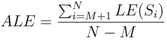
The performance metric used to evaluate the performance of different localization schemes is the average localization error for all unknown sensor nodes,
ALE,
where
N is the total number of sensor nodes,
M is the number of beacon nodes, and
LE(
Si) is the localization error of the sensor node
Si,
The parameters used in the simulation study are summarized in
Table 1.
Table 1.
Simulation Parameters.
Table 1.
Simulation Parameters.
| Parameter | Value |
|---|
| Number of Sensor Nodes, N | 150/200/250/300/350/400 |
| Beacon Ratio | 0.1–0.3 |
| Sensor Field Size | 50 m× 50 m |
| Transmission Range of a Sensor Node, r | 10 m |
| Number of Component NN, K | 7 |
4.1. Performance Comparison
The performance of the proposed LNNE system is compared with two well-known range-free localization algorithms, Centroid and DV-Hop, as well as the localization algorithm based on signal neural network, LSNN.
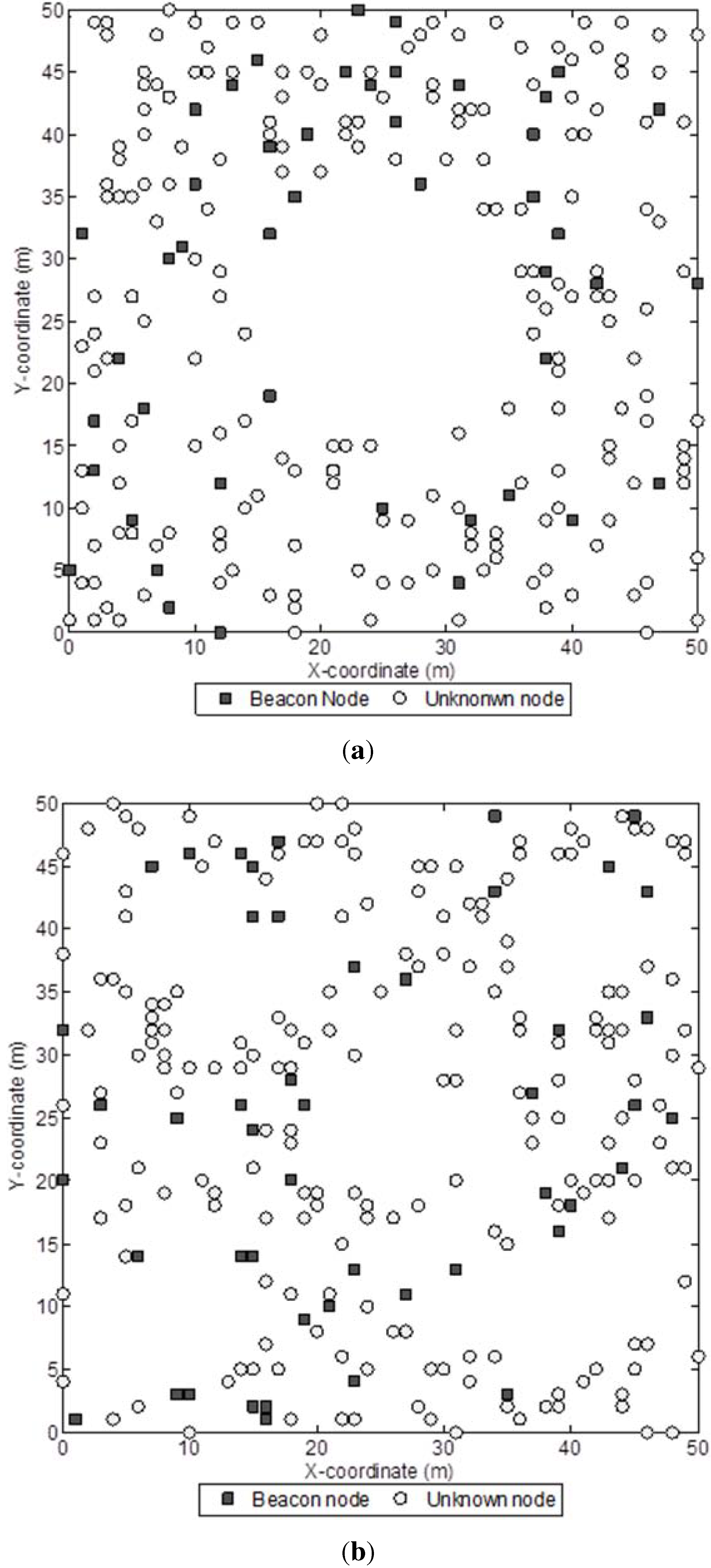
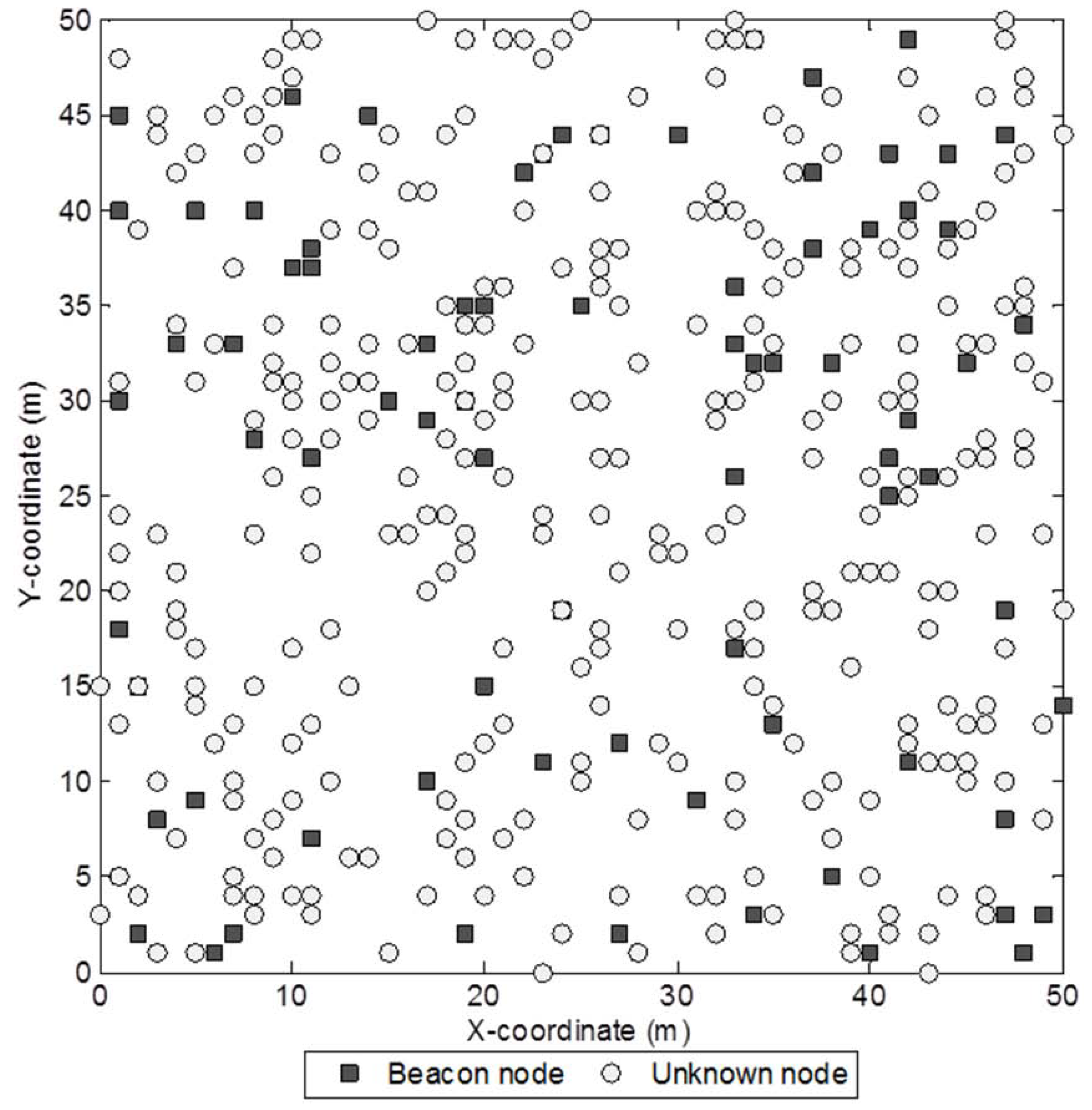
Figure 3.
Sample network with 400 sensor nodes and a beacon ratio of 0.2.
Figure 3.
Sample network with 400 sensor nodes and a beacon ratio of 0.2.
4.1.1. Effects of Beacon Ratio and Network Density
In the first two studies, the sensor nodes are uniformly placed in the field without coverage hole.
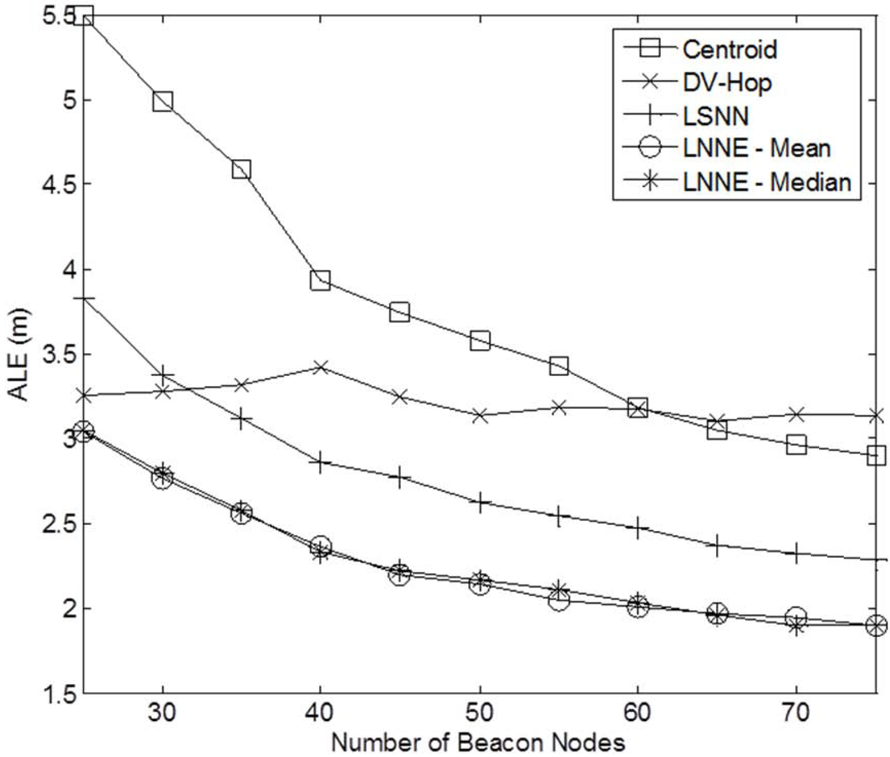
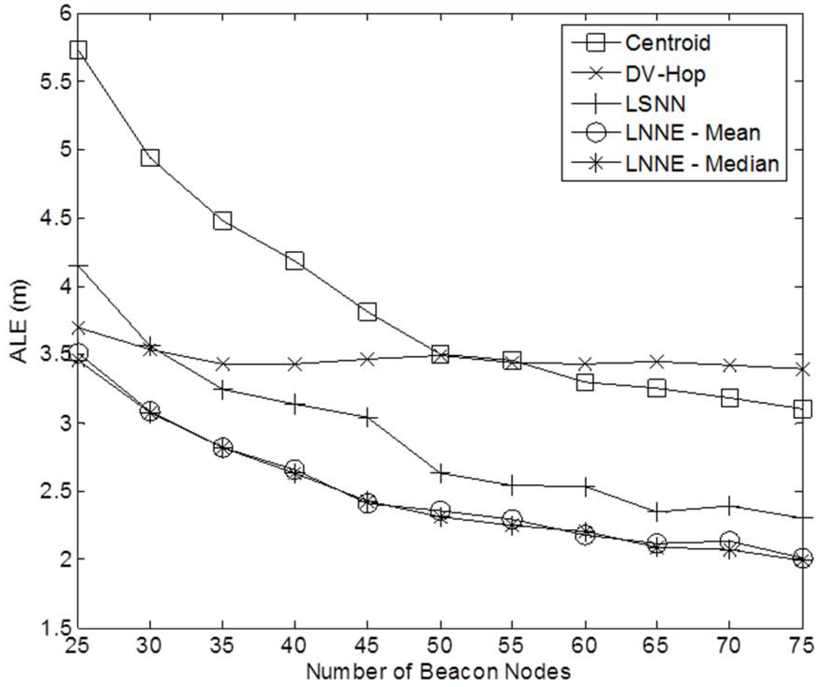
Figure 3 shows a sample network with 400 sensor nodes and a beacon ratio of 0.2. We first investigate the effect of beacon ratio on the performance of the four localization algorithms. The number of sensor nodes in the field is set to 250. The number of beacon nodes varies from 25 to 75, which corresponds to a beacon ratio of 0.1 to 0.3. The simulation results are shown in
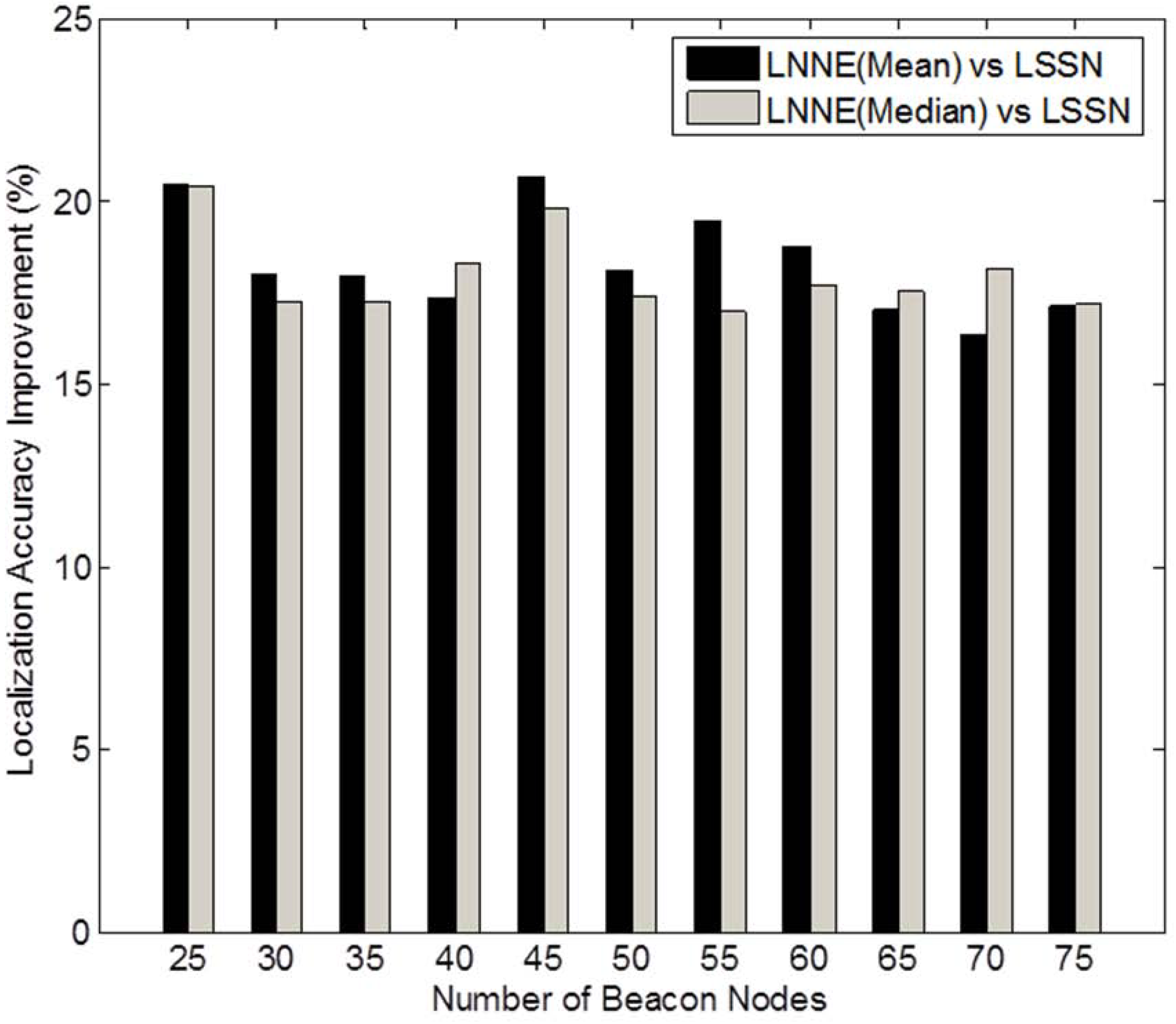
Figure 4. Generally, the localization errors of the four algorithms are decreased with the increment of beacon ratio. The proposed LNNE outperforms other three algorithms in all cases. For LNNE, the two combination rules, mean rule and median rule, produce comparable results. Compared with LSNN, LNNE can improve the localization accuracy up to 20.7% as shown in
Figure 5.
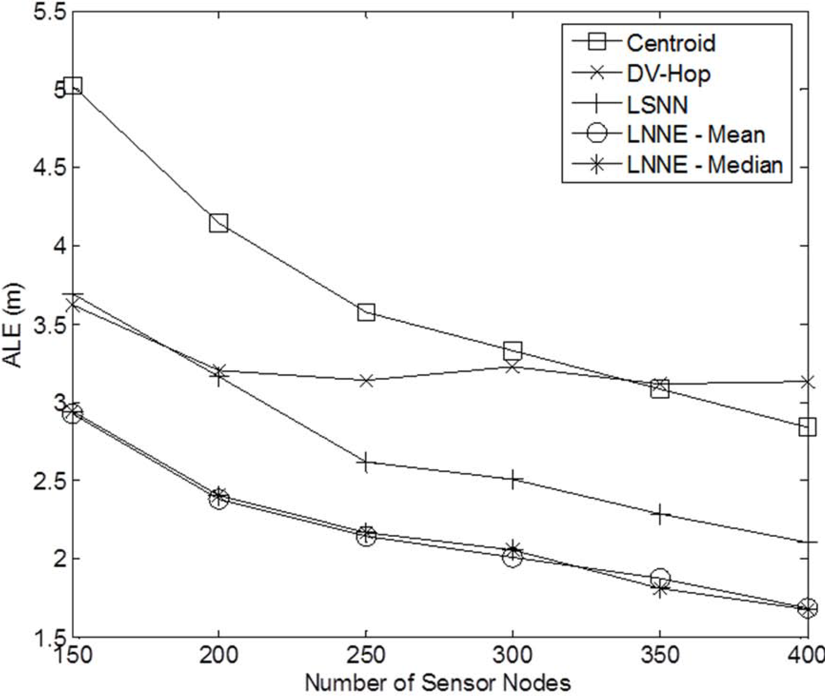
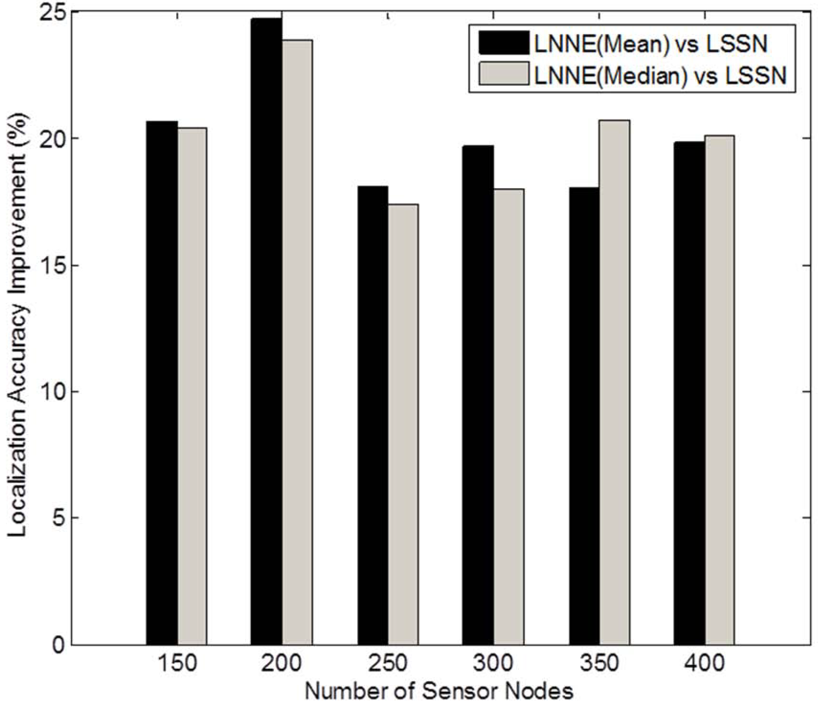
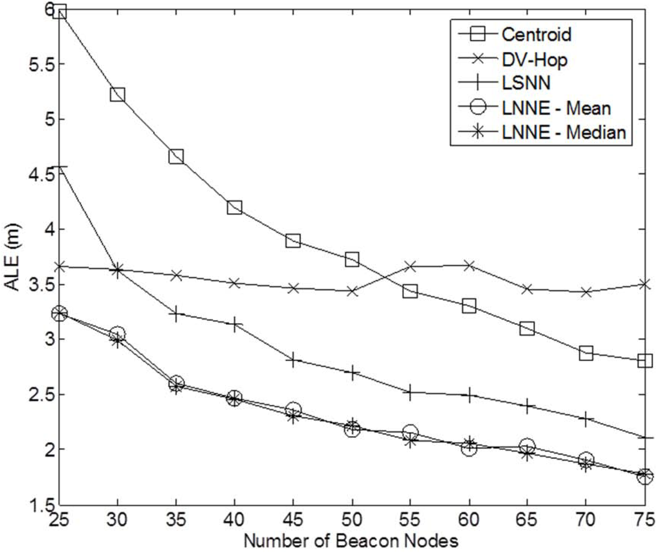
Next, the effect of network density on the performance of the localization algorithms is studied. The network density is changed by varying the number of sensor nodes in the field. In the simulation, the number of sensor nodes,
N , varies from 150 to 400 while the beacon ratio is fixed at 0.2.
Figure 6 shows the simulation results. Better localization accuracy can be observed for a denser network. For all cases, the proposed LNNE has the best performance. Similar to the previous experiment, the mean rule and median rule achieve comparable results for LNNE. As shown in
Figure 7, LNNE significantly improves the localization accuracy compared with LSNN with an average improvement of more than 20%.
Figure 4.
Performance comparison among different beacon ratios (N =250, beacon ratio=0.1–0.3, no coverage holes).
Figure 4.
Performance comparison among different beacon ratios (N =250, beacon ratio=0.1–0.3, no coverage holes).
Figure 5.
Performance improvement of LNNE vs. LSSN (N = 250, beacon ratio = 0.1–0.3, no coverage holes).
Figure 5.
Performance improvement of LNNE vs. LSSN (N = 250, beacon ratio = 0.1–0.3, no coverage holes).
Figure 6.
Performance comparison among different network densities (N = 150 to 400, beacon ratio = 0.2, nocoverage holes).
Figure 6.
Performance comparison among different network densities (N = 150 to 400, beacon ratio = 0.2, nocoverage holes).
Figure 7.
Performance improvement of LNNE vs. LSSN under different network densities (N = 150 to 400, beacon ratio = 0.2, no coverage holes).
Figure 7.
Performance improvement of LNNE vs. LSSN under different network densities (N = 150 to 400, beacon ratio = 0.2, no coverage holes).
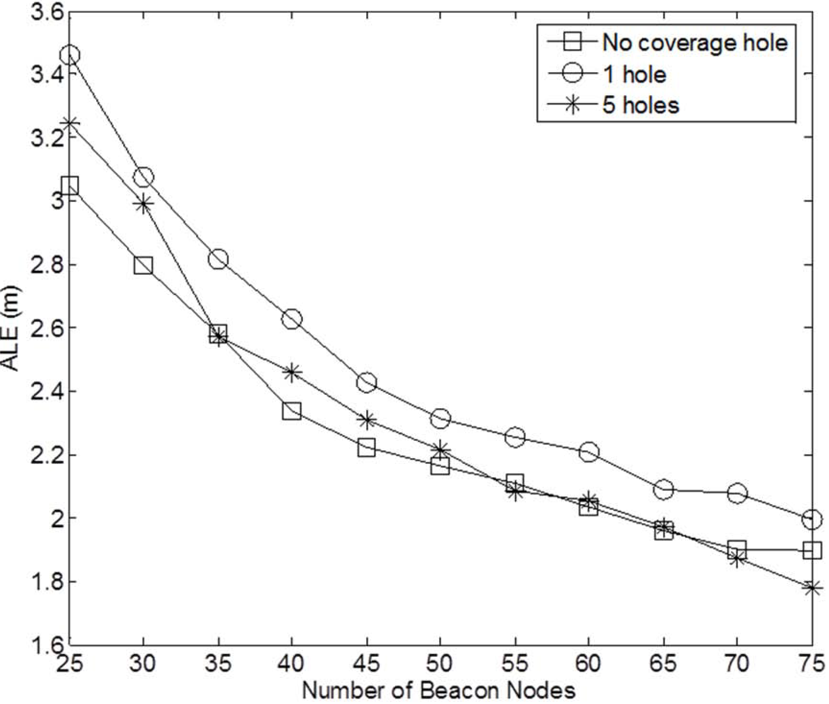
4.1.2. Effects of Coverage Holes
Due to the obstacles in the sensor field, there are normally coverage holes in the sensor network. Similar to [
15,
17], we consider two cases: (1) one circular hole centered at (25, 25) with the radius of 10
m; (2) five circular holes with the radius of 5
m centered at (25, 25), (10, 10), (10, 40), (40, 10), and (40, 40), respectively. In this experiment, we consider networks with 250 sensor nodes and the beacon ratio varying from 0.1 to 0.3.Sample networks for the two cases with a beacon ratio of 0.2 are shown in
Figure 8.
Figure 9 and
Figure 10 show the performance of the four localization algorithms for the two coverage hole cases, respectively. Similar to the case of no coverage hole in the network, LNNE achieves significantly better performance than other three localization algorithms. The two combination rules of LNNE produce comparable results. The effect of the coverage holes on the performance of LNNE (median rule) is shown in
Figure 11. It can be observed that the performance of LNNE degrades in most cases because of the coverage holes, especially in the cases that a large coverage hole (obstacle) in the network or the beacon ratio is low. However, LNNE still maintains high localization accuracy as shown
Figure 9 and
Figure 10.
Figure 8.
Sample networks with coverage holes (250 sensor nodes and 50 beacon nodes):(a) 1 hole; (b) 5 holes.
Figure 8.
Sample networks with coverage holes (250 sensor nodes and 50 beacon nodes):(a) 1 hole; (b) 5 holes.
Figure 9.
Performance comparison under different beacon ratios (0.1-0.3) and 1 coverage hole.
Figure 9.
Performance comparison under different beacon ratios (0.1-0.3) and 1 coverage hole.
Figure 10.
Performance comparison under different beacon ratios (0.1-0.3) and 5 coverage holes.
Figure 10.
Performance comparison under different beacon ratios (0.1-0.3) and 5 coverage holes.
Figure 11.
Effect of coverage holes on LNNE (N = 250, beacon ratio = 0.1-0.3).
Figure 11.
Effect of coverage holes on LNNE (N = 250, beacon ratio = 0.1-0.3).
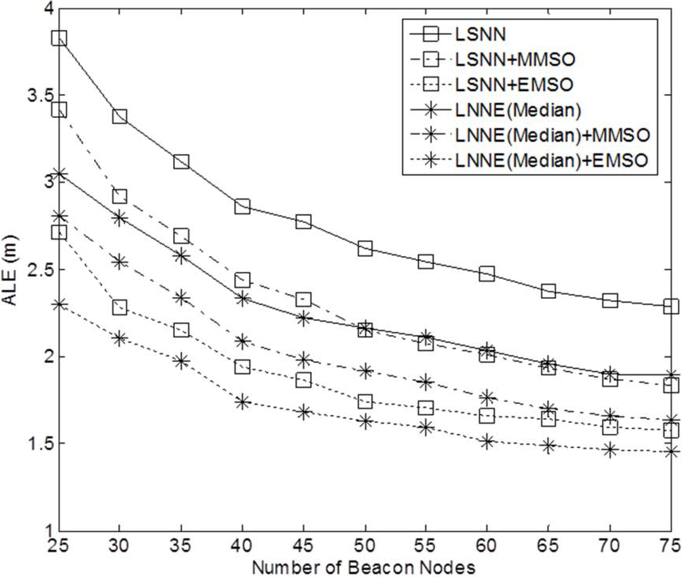
Figure 12.
Performance of refinement algorithms under different beacon ratios (N = 250, beacon ratio = 0.1-0.3, no coverage holes).
Figure 12.
Performance of refinement algorithms under different beacon ratios (N = 250, beacon ratio = 0.1-0.3, no coverage holes).
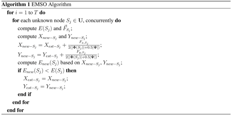
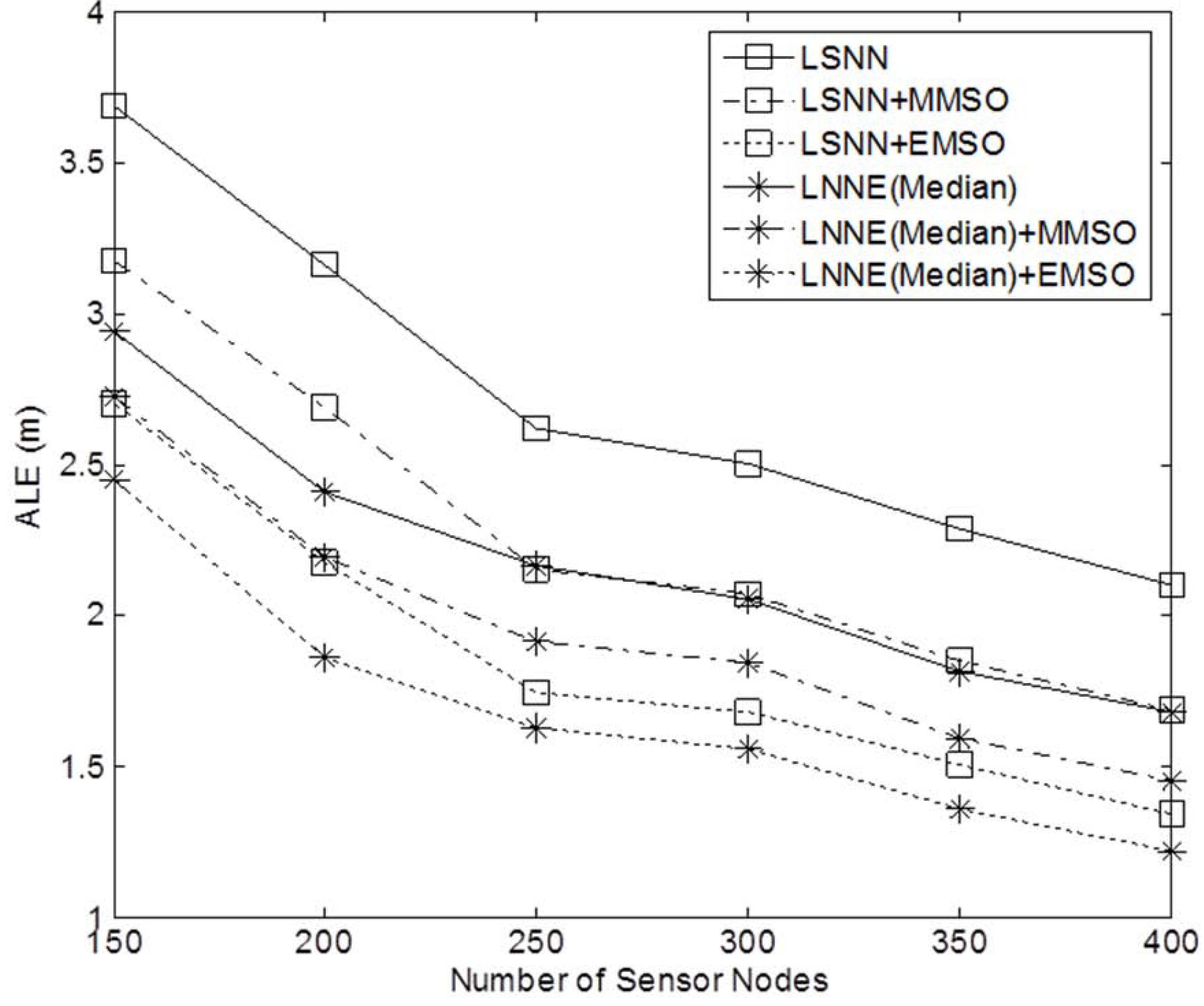
4.2. Improving Localization Accuracy with EMSO Algorithm
The performance of the refinement algorithms is also investigated. We study the effect of MMSO and EMSO on the performance of LSNN and LNNE. Only median rule is considered for LNNE since the mean rule produces comparable result as shown in
Section 4.1. The maximum number of iterations for MMSO and EMSO is 100. The simulation results for networks without coverage holes are shown in
Figure 12 and
Figure 13. The results demonstrate that MMSO can significantly improve the performance of LSNN and LNNE. EMSO can further improve the localization accuracy by utilizing the location information of the neighboring beacon and unknown nodes. The combination of LNNE and EMSO consistently achieves the best performance. With EMSO, the performance of LNNE can be improved by 24% on average, compared with an average improvement of 11% by MMSO.
Figure 13.
Performance of refinement algorithms with different network densities (N = 150 to 400, beacon ratio = 0.2, no coverage holes).
Figure 13.
Performance of refinement algorithms with different network densities (N = 150 to 400, beacon ratio = 0.2, no coverage holes).
5. Conclusions
In this paper, neural network ensembles are used to improve the localization accuracy for WSNs by utilizing the diversity of the component neural networks. The localization system, LNNE, only utilize the connectivity information of the network to estimate the location of sensor nodes. Simulation studies are carried out to compare the performance of LNNE with two well-known range-free localization algorithms, Centroid and DV-Hop, and a single neural network-based localization algorithm, LSNN. The effects of beacon ratio, network density, and coverage holes on the performance of LNNE are investigated. The experimental results demonstrate that LNNE outperforms other three algorithms in all simulation cases. The EMSO algorithm is also proposed, which can significantly improve the performance of LNNE with the help of location information of the neighboring beacon and unknown nodes.


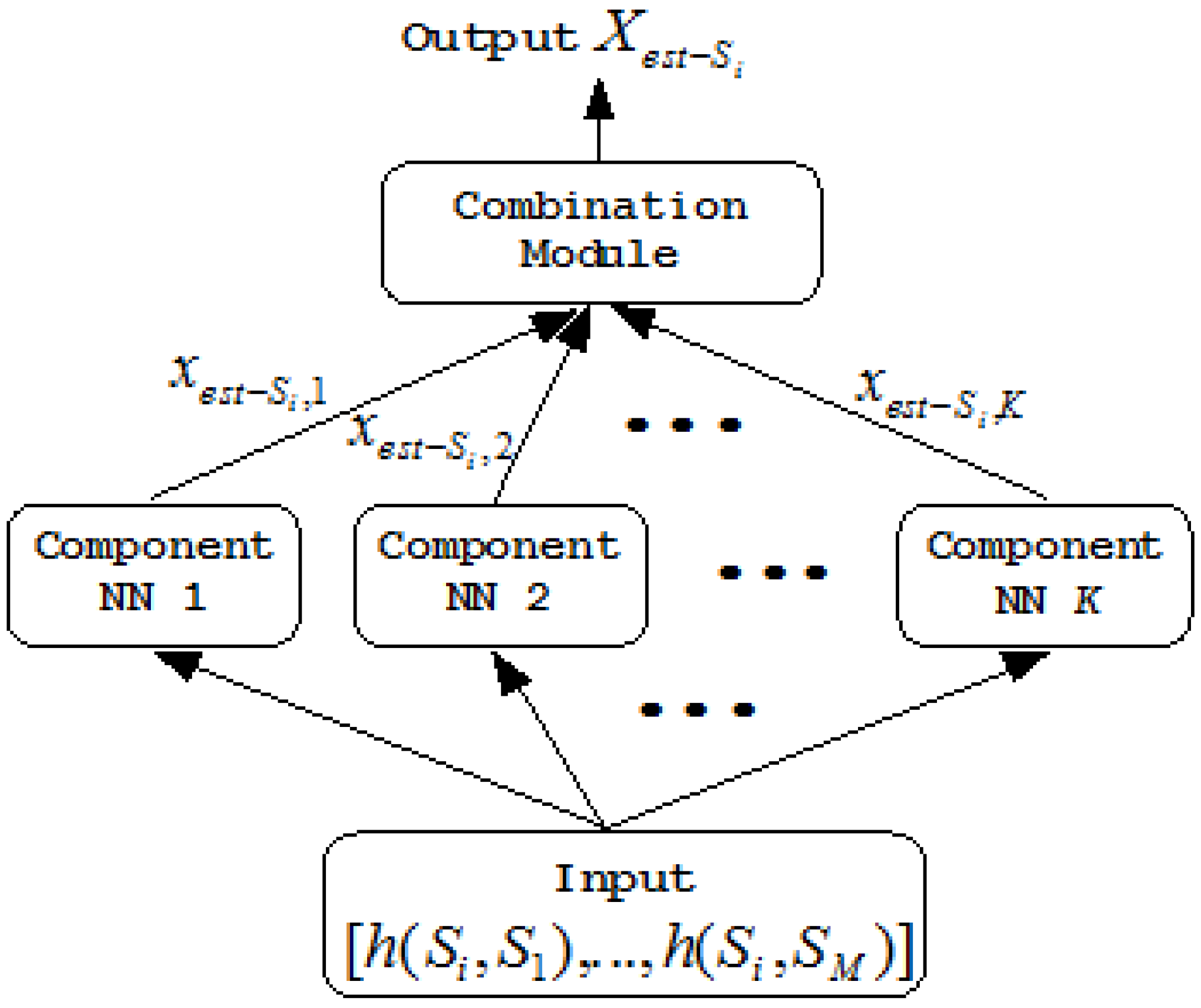
 ). Each component neural network has the same architecture. Figure 2 shows an example of the kth component neural network for X -NNE.
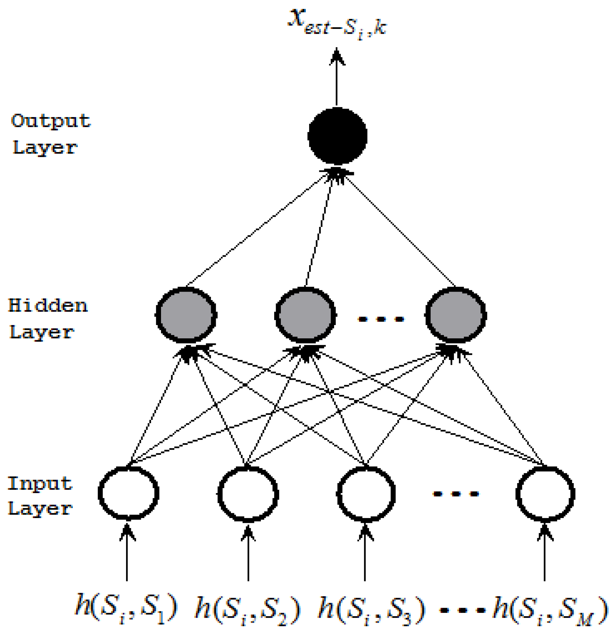
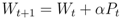


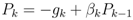
 , where E(Si) is the energy of a sensor node Si defined as
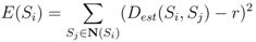
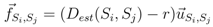
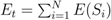
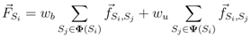
 is the unit vector from Si to Sj. When computing the total force applied on the sensor node Si pulled by all 1-hop neighboring nodes, we give a higher weight to the beacon node as the location of beacon node is known. The total force on Si is then defined as

