
Fall and Winter Temperatures, Together with Spring Temperatures, Determine the First Flowering Date of Prunus armeniaca L.

 , , and
Abstract
1. Introduction
2. Materials and Methods
2.1. First Flowering Date Records and Climate Data
2.2. Methods for Quantifying the Effect of Spring Temperatures on Phenological Occurrence Date
2.2.1. Accumulated Degree Days (ADD) Method
2.2.2. Accumulated Days Transferred to a Standardized Temperature (ADTS) Method
2.2.3. Accumulated Developmental Progress (ADP) Method
2.3. Methods for Quantifying the Effect of Fall and Winter Temperatures (FWTs) on Occurrence Date
3. Results
4. Discussion
4.1. Two Other Nonlinear Equations for Describing Temperature-Dependent Developmental Rate
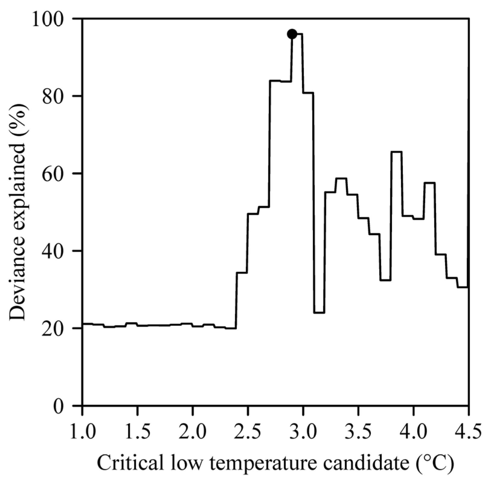
4.2. Influence of the Upper Threshold Temperature in the Chilling Hours Model on Goodness of Fit
4.3. Effect of Daily Maximum Temperatures on Occurrence Date
4.4. Overlap Between Chilling and Heat Accumulation: Implications for Phenological Modeling
4.5. Strengths and Limitations of the Methods Presented Here
5. Conclusions
Author Contributions
Funding
Data Availability Statement
Acknowledgments
Conflicts of Interest
References
- Chmielewski, F.M. Phenology and agriculture. In Phenology: An Integrative Environmental Science. Tasks for Vegetation Science; Schwartz, M.D., Ed.; Springer: Dordrecht, The Netherlands, 2003; Volume 39, pp. 539–561. [Google Scholar]
- Schwartz, M.D. Phenology: An Integrative Environmental Science, 3rd ed.; Springer: Berlin/Heidelberg, Germany, 2025. [Google Scholar]
- Chuine, I.; Morin, X.; Bugmann, H. Warming, photoperiods, and tree phenology. Science 2010, 329, 277–278. [Google Scholar] [CrossRef] [PubMed]
- Fu, Y.H.; Zhao, H.; Piao, S.; Peaucelle, M.; Peng, S.; Zhou, G.; Ciais, P.; Huang, M.; Menzel, A.; Peñuelas, J.; et al. Declining global warming effects on the phenology of spring leaf unfolding. Nature 2015, 526, 104–107. [Google Scholar] [CrossRef] [PubMed]
- Prevéy, J.S.; Rixen, C.; Rüger, N.; Høye, T.T.; Bjorkman, A.D.; Myers-Smith, I.H.; Elmendorf, S.C.; Ashton, I.W.; Cannone, N.; Chisholm, C.L.; et al. Warming shortens flowering seasons of tundra plant communities. Nat. Ecol. Evol. 2019, 3, 45–52. [Google Scholar] [CrossRef] [PubMed]
- Visser, M.E.; Gienapp, P. Evolutionary and demographic consequences of phenological mismatches. Nat. Ecol. Evol. 2019, 3, 879–885. [Google Scholar] [CrossRef]
- Heide, O.M. High autumn temperature delays spring bud burst in boreal trees, counterbalancing the effect of climatic warming. Tree Physiol. 2003, 23, 931–936. [Google Scholar] [CrossRef]
- Linvill, D.E. Calculating chilling hours and chill units from daily maximum and minimum temperature observations. HortScience 1990, 25, 14–16. [Google Scholar] [CrossRef]
- Luedeling, E.; Zhang, M.; Luedeling, V.; Girvetz, E.H. Sensitivity of winter chill models for fruit and nut trees to climatic changes expected in California’s Central Valley. Agric. Ecosyst. Environ. 2009, 133, 23–31. [Google Scholar] [CrossRef]
- Fu, Y.H.; Campioli, M.; Deckmyn, G.; Janssens, I.A. The impact of winter and spring temperatures on temperate tree budburst dates: Results from an experimental climate manipulation. PLoS ONE 2012, 7, e47324. [Google Scholar] [CrossRef]
- Shi, P.; Chen, Z.; Reddy, G.V.P.; Hui, C.; Huang, J.; Xiao, M. Timing of cherry tree blooming: Contrasting effects of rising winter low temperatures and early spring temperatures. Agric. Forest Meteorol. 2017, 240−241, 78–89. [Google Scholar] [CrossRef]
- Shi, P.; Fan, M.; Reddy, G.V.P. Comparison of thermal performance equations in describing temperature-dependent developmental rates of insects: (III) Phenological applications. Ann. Entomol. Soc. Am. 2017, 110, 558–564. [Google Scholar] [CrossRef]
- Zhang, R.; Lin, J.; Wang, F.; Delpierre, N.; Kramer, K.; Hänninen, H.; Wu, J. Spring phenology in subtropical trees: Developing process-based models on an experimental basis. Agric. Forest Meteorol. 2022, 314, 108802. [Google Scholar] [CrossRef]
- Chuine, I. A unified model for budburst of trees. J. Theor. Biol. 2000, 207, 337–347. [Google Scholar] [CrossRef] [PubMed]
- Chuine, I.; Bonhomme, M.; Legave, J.-M.; de Cortázar-Atauri, I.G.; Charrier, G.; Lacointe, A. Can phenological models predict tree phenology accurately in the future? The unrevealed hurdle of endodormancy break. Glob. Change Biol. 2016, 22, 3444–3460. [Google Scholar] [CrossRef]
- Kramer, K. Selecting a model to predict the onset of growth of Fagus sylvatica. J. Appl. Ecol. 1994, 31, 172–181. [Google Scholar] [CrossRef]
- Luedeling, E.; Kunz, A.; Blanke, M. Identification of chilling and heat requirements of cherry trees—A statistical approach. Int. J. Biometeorol. 2013, 57, 679–689. [Google Scholar] [CrossRef]
- Ruiz, D.; Campoy, J.A.; Egea, J.A. Chilling and heat requirements of apricot cultivars for flowering. Environ. Exp. Bot. 2007, 61, 254–263. [Google Scholar] [CrossRef]
- Delgado, A.; Ruiz, D.; Munoz-Morales, A.M.; Campoy, J.A.; Egea, J.A. Analysing variations in flowering time based on the dynamics of chill and heat accumulation during the fulfilment of cultivar-specific chill requirements in apricot. Eur. J. Agron. 2025, 164, 127509. [Google Scholar] [CrossRef]
- Shi, P.; Reddy, G.V.P.; Chen, L.; Ge, F. Comparison of thermal performance equations in describing temperature-dependent developmental rates of insects: (I) empirical models. Ann. Entomol. Soc. Am. 2016, 109, 211–215. [Google Scholar] [CrossRef]
- Shi, P.; Quinn, B.K.; Zhang, Y.; Bao, X.; Lin, S. Comparison of the intrinsic optimum temperatures for seed germination between two bamboo species based on a thermodynamic model. Glob. Ecol. Conser. 2019, 17, e00568. [Google Scholar] [CrossRef]
- Quinn, B.K. A critical review of the use and performance of different function types for modeling temperature-dependent development of arthropod larvae. J. Therm. Biol. 2017, 63, 65–77. [Google Scholar] [CrossRef]
- Uvarov, B.P. Insects and climate. Trans. Entomol. Soc. Lond. 1931, 79, 1–232. [Google Scholar] [CrossRef]
- Campbell, A.; Frazer, B.D.; Gilbert, N.; Gutierrez, A.P.; Mackauer, M. Temperature requirements of some aphids and their parasites. J. Appl. Ecol. 1974, 11, 431–438. [Google Scholar] [CrossRef]
- Sharpe, P.J.H.; DeMichele, D.W. Reaction kinetics of poikilotherm development. J. Theor. Biol. 1977, 64, 649–670. [Google Scholar] [CrossRef] [PubMed]
- Ratkowsky, D.A.; Reddy, G.V.P. Empirical model with excellent statistical properties for describing temperature-dependent developmental rates of insects and mites. Ann. Entomol. Soc. Am. 2017, 110, 302–309. [Google Scholar] [CrossRef]
- Rebaudo, F.; Struelens, Q.; Dangles, O. Modelling temperature-dependent development rate and phenology in arthropods: The devRate package for R. Methods Ecol. Evol. 2017, 9, 1144–1150. [Google Scholar] [CrossRef]
- Logan, J.A.; Wollkind, D.J.; Hoyt, S.C.; Tanigoshi, L.K. An analytic model for description of temperature dependent rate phenomena in arthropods. Environ. Entomol. 1976, 5, 1133–1140. [Google Scholar] [CrossRef]
- Davidson, J. On the relationship between temperature and rate of development of insects at constant temperatures. J. Anim. Ecol. 1944, 13, 26–38. [Google Scholar] [CrossRef]
- Hänninen, H. Modelling bud dormancy release in trees from cool and temperate regions. Acta For. Fenn. 1990, 213, 1–47. [Google Scholar] [CrossRef]
- Wagner, T.L.; Wu, H.-I.; Sharpe, P.J.H.; Schoolfield, R.M.; Coulson, R.N. Modelling insect development rates: A literature review and application of a biophysical model. Ann. Entomol. Soc. Am. 1984, 77, 208–220. [Google Scholar] [CrossRef]
- Ring, D.R.; Harris, M.K. Predicting pecan nut casebearer (Lepidoptera: Pyralidae) activity at College Station, Texas. Environ. Entomol. 1983, 12, 482–486. [Google Scholar] [CrossRef]
- Aono, Y. Climatological studies on blooming of cherry tree (Prunus yedoensis) by means of DTS method. Bull. Univ. Osaka Pref. Ser. B Agric. Life Sci. 1993, 45, 155–192, (In Japanese with English Abstract). [Google Scholar]
- Guo, L.; Xu, J.; Dai, J.; Cheng, J.; Luedeling, E. Statistical identification of chilling and heat requirements for apricot flower buds in Beijing, China. Sci. Horticul. 2015, 195, 138–144. [Google Scholar] [CrossRef]
- Shi, P.; Chen, Z.; Quinn, B.K. spphpr: Spring Phenological Prediction; R Package Version 1.1.4; The Comprehensive R Archive Network (CRAN): Vienna, Austria, 2025. [Google Scholar]
- Ring, D.R. Predicting Biological Events in the Life History of the Pecan Nut Casebearer Using a Degree Day Model. Ph.D. Thesis, Texas A&M University, College Station, TX, USA, 1981. [Google Scholar]
- Konno, T.; Sugihara, S. Temperature index for characterizing biological activity in soil and its application to decomposition of soil organic matter. Bull. Natl. Inst. Agro-Environ. Sci. 1986, 1, 51–68, (In Japanese with English Abstract). [Google Scholar]
- Ungerer, M.J.; Ayres, M.P.; Lombardero, M.J. Climate and the northern distribution limits of Dendroctonus frontalis Zimmermann (Coleoptera: Scolytidae). J. Biogeogr. 1999, 26, 1133–1145. [Google Scholar] [CrossRef]
- Nelder, J.A.; Mead, R. A simplex method for function minimization. Comput. J. 1965, 7, 308–313. [Google Scholar] [CrossRef]
- Hastie, T.J.; Tibshirani, R.J. Generalized additive models (with discussion). Stat. Sci. 1986, 1, 297–318. [Google Scholar]
- Hastie, T.J.; Tibshirani, R.J. Generalized Additive Models; Chapman and Hall: London, UK, 1990. [Google Scholar]
- Wood, S.N. Generalized Additive Models: An Introduction with R, 2nd ed.; Chapman and Hall/CRC Press: New York, NY, USA, 2017. [Google Scholar]
- Akaike, H. Information theory and an extension of the maximum likelihood principle. In Selected Papers of Hirotugu Akaike; Parzen, E., Tanabe, K., Kitagawa, G., Eds.; Springer: New York, NY, USA, 1998; pp. 199–213. [Google Scholar]
- Spiess, A.N.; Neumeyer, N. An evaluation of R2 as an inadequate measure for nonlinear models in pharmacological and biochemical research: A Monte Carlo approach. BMC Pharmacol. 2010, 10, 6. [Google Scholar] [CrossRef]
- Chandler, W.H. Deciduous Orchards; Lea & Febiger: Philadelphia, PA, USA, 1942. [Google Scholar]
- Luedeling, E.; Brown, P.H. A global analysis of the comparability of winter chill models for fruit and nut trees. Int. J. Biometeorol. 2011, 55, 411–421. [Google Scholar] [CrossRef]
- Zohner, C.M.; Mo, L.; Sebald, V.; Renner, S.S. Leaf-out in northern ecotypes of wide-ranging trees requires less spring warming, enhancing the risk of spring frost damage at cold limits. Glob. Ecol. Biogeogr. 2020, 29, 1065–1072. [Google Scholar] [CrossRef]
- Yang, Y.; Ratkowsky, D.A.; Yang, J.; Shi, P. Effects of plant coverage on the abundance of adult mosquitos at an urban park. Plants 2023, 12, 983. [Google Scholar] [CrossRef]
- R Core Team. R: A Language and Environment for Statistical Computing; R Foundation for Statistical Computing: Vienna, Austria, 2023; Available online: https://www.r-project.org/ (accessed on 26 July 2023).
- Wood, S.N. Fast stable restricted maximum likelihood and marginal likelihood estimation of semiparametric generalized linear models. J. R. Statist. Soc. B 2011, 73, 3–36. [Google Scholar] [CrossRef]
- Zhang, R.; Lin, J.; Wang, F.; Shen, S.; Wang, X.; Rao, Y.; Wu, J.; Hänninen, H. The chilling requirement of subtropical trees is fulfilled by high temperatures: A generalized hypothesis for tree endodormancy release and a method for testing it. Agric. Forest Meteorol. 2021, 298–299, 108296. [Google Scholar] [CrossRef]
- Sarvas, R. Investigations on the annual cycle of development of forest trees. II. Autumn dormancy and winter dormancy. Commun. Inst. Fiorestalis Fenn. 1974, 84, 1–101. [Google Scholar]
- Wang, J.; Xi, Z.; He, X.; Chen, S.; Rossi, S.; Smith, N.G.; Liu, J.; Chen, L. Contrasting temporal variations in responses of leaf unfolding to daytime and nighttime warming. Glob. Change Biol. 2021, 27, 5084–5093. [Google Scholar] [CrossRef]
- Wang, J.; Hua, H.; Guo, J.; Huang, X.; Zhang, X.; Yang, Y.; Wang, D.; Guo, X.; Zhang, R.; Smith, N.G.; et al. Late spring frost delays tree spring phenology by reducing photosynthetic productivity. Nat. Clim. Change 2025, 15, 201–209. [Google Scholar] [CrossRef]
- Meng, L.; Zhou, Y.; Gu, L.; Richardson, A.D.; Peñuelas, J.; Fu, Y.; Wang, Y.; Asrar, G.R.; de Boeck, H.J.; Mao, J.; et al. Photoperiod decelerates the advance of spring phenology of six deciduous tree species under climate warming. Glob. Change Biol. 2021, 27, 2914–2927. [Google Scholar] [CrossRef]


| Formula | AIC | Deviance Explained | Non-Significant Items |
|---|---|---|---|
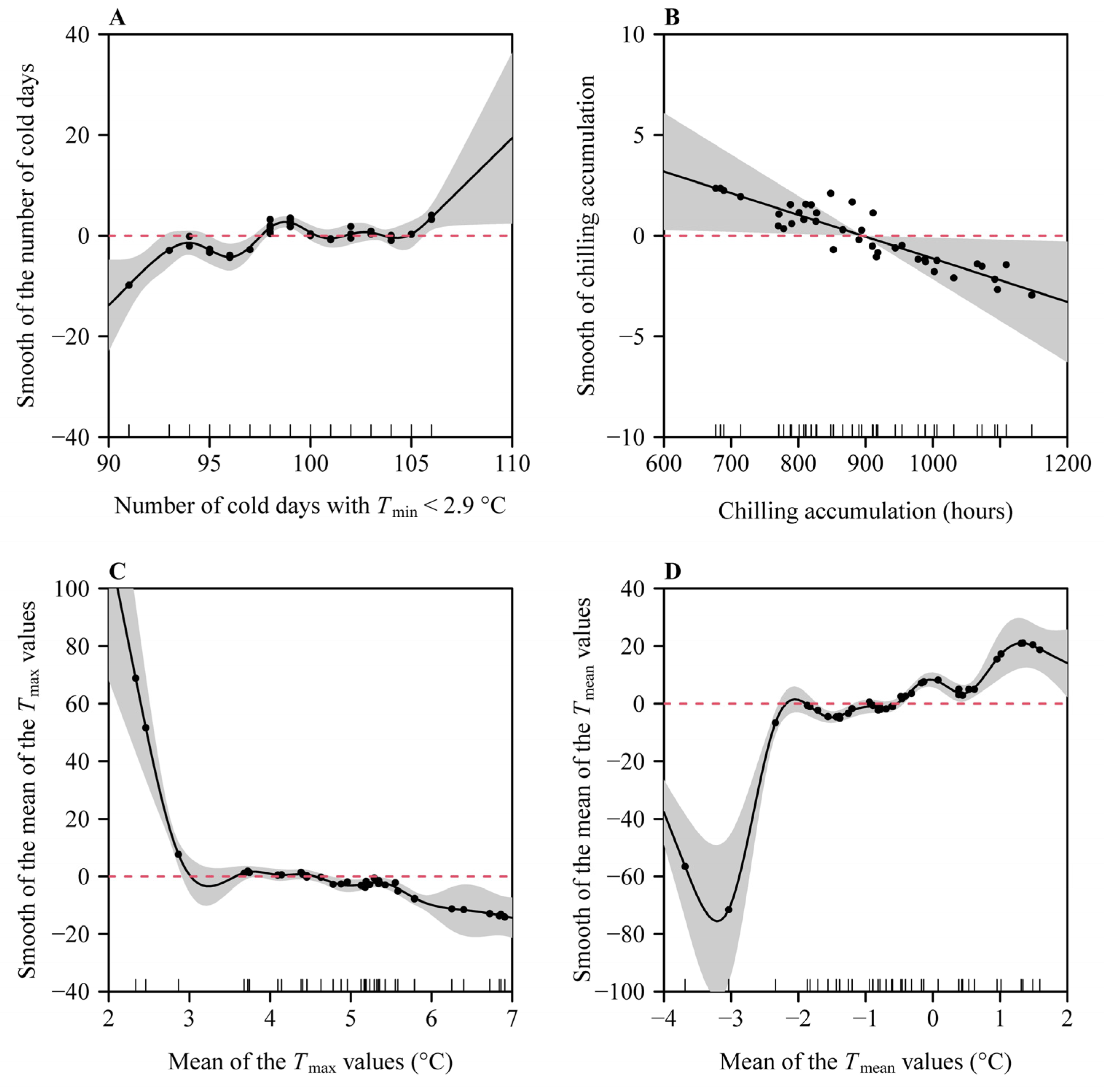
| y ~ s(x1) + s(x2) + s(x3) + s(x4) + s(x5) + s(x6) | 86.62 | 99.0% | s(x3) |
| y ~ + s(x2) + s(x3) + s(x4) + s(x5) + s(x6) | 203.56 | 42.1% | All items |
| y ~ s(x1) + s(x3) + s(x4) + s(x5) + s(x6) | 127.28 | 96.6% | s(x4) and s(x6) |
| y ~ s(x1) + s(x2) + s(x4) + s(x5) + s(x6) | 167.26 | 86.5% | s(x6) |
| y ~ s(x1) + s(x2) + s(x3) + s(x5) + s(x6) | 192.08 | 64.5% | s(x5) and s(x6) |
| y ~ s(x1) + s(x2) + s(x3) + s(x4) + s(x6) | 200.05 | 39.0% | s(x1), s(x2), s(x4), and s(x6) |
| y ~ s(x1) + s(x2) + s(x3) + s(x4) + s(x5) | 161.09 | 89.6% | s(x2) and s(x3) |
| y ~ s(x1) + s(x2) + s(x4) + s(x5) | 130.02 | 96.0% | − |
| y ~ s(x1) + s(x2) + s(x5) | 202.52 | 26.8% | All items |
| y ~ s(x1) + s(x2) + s(x4) | 205.80 | 17.6% | All items |
| Method | Estimate of the Starting Date (DOY) | Estimate(s) of the Model Parameter(s) | RMSE (Days) |
|---|---|---|---|
| ADD | 65 | T0 = −0.52 °C | 3.1189 |
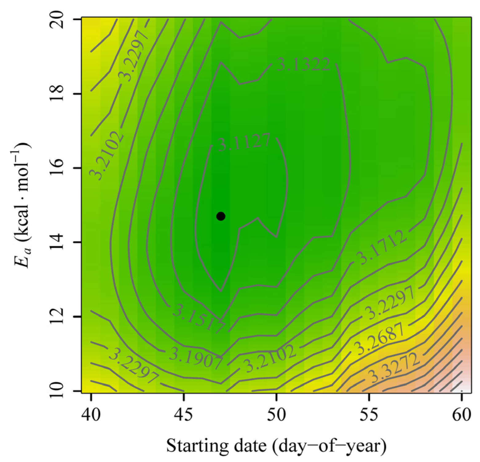
| ADTS | 47 | Ea = 14.7 kcal∙mol−1 | 3.0932 |
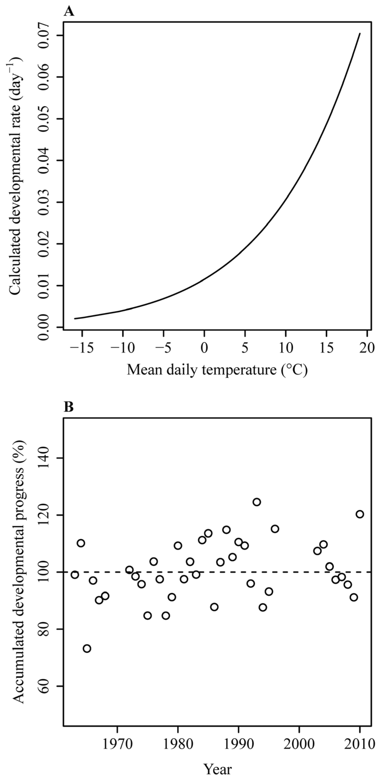
| ADP–Arrhenius | 47 | B = −4.38 | 3.090395 |
| Ea = 15.04 kcal∙mol−1 | |||
| ADP–Logan | 47 | ψ = 0.01226 | 3.090418 |
| ρ = 0.1066 | |||
| Tu = 40.63 | |||
| z = 5.8179 | |||
| ADP–Logistic | 47 | K = 0.1463 | 3.088134 |
| K0 = 0.0114 | |||
| b = 0.1148 |
Disclaimer/Publisher’s Note: The statements, opinions and data contained in all publications are solely those of the individual author(s) and contributor(s) and not of MDPI and/or the editor(s). MDPI and/or the editor(s) disclaim responsibility for any injury to people or property resulting from any ideas, methods, instructions or products referred to in the content. |
© 2025 by the authors. Licensee MDPI, Basel, Switzerland. This article is an open access article distributed under the terms and conditions of the Creative Commons Attribution (CC BY) license (https://creativecommons.org/licenses/by/4.0/).
Share and Cite
Tang, D.; Quinn, B.K.; Yang, Y.; Guo, L.; Ratkowsky, D.A.; Shi, P. Fall and Winter Temperatures, Together with Spring Temperatures, Determine the First Flowering Date of Prunus armeniaca L. Plants 2025, 14, 1503. https://doi.org/10.3390/plants14101503
Tang D, Quinn BK, Yang Y, Guo L, Ratkowsky DA, Shi P. Fall and Winter Temperatures, Together with Spring Temperatures, Determine the First Flowering Date of Prunus armeniaca L. Plants. 2025; 14(10):1503. https://doi.org/10.3390/plants14101503
Chicago/Turabian StyleTang, Di, Brady K. Quinn, Yunfeng Yang, Liang Guo, David A. Ratkowsky, and Peijian Shi. 2025. "Fall and Winter Temperatures, Together with Spring Temperatures, Determine the First Flowering Date of Prunus armeniaca L." Plants 14, no. 10: 1503. https://doi.org/10.3390/plants14101503
APA StyleTang, D., Quinn, B. K., Yang, Y., Guo, L., Ratkowsky, D. A., & Shi, P. (2025). Fall and Winter Temperatures, Together with Spring Temperatures, Determine the First Flowering Date of Prunus armeniaca L. Plants, 14(10), 1503. https://doi.org/10.3390/plants14101503