Abstract
(1) Background: Boreal forests influence global carbon balance and fulfil multiple ecosystem services. Their vegetation growth and biomass are significantly affected by environmental conditions. In the present study we focused on one of the least accessible and least studied parts of the boreal region situated in the western part of Putorana plateau, Central Siberia (Lama and Keta lakes, Krasnoyarsk region), northern Russia. (2) Methods: We derived local height-diameter and crown radius-height models for six tree species. We used univariate correlation and multiple regression analyses to examine the relationships between tree biomass and environmental conditions. (3) Results: Total tree biomass stock (aboveground tree biomass + aboveground and buried deadwood) varied between 6.47 t/ha and 149 t/ha, while total deadwood biomass fluctuated from 0.06 to 21.45 t/ha. At Lama, biomass production decreased with elevation. At Keta, the relationship of biomass to elevation followed a U shape. Stand biomass changed with micro-terrain morphology and soil nutrient content, while the patterns were location-specific. (4) Conclusions: The majority of the derived models were significant and explained most of the variability in the relationships between tree diameter or crown radius and tree height. Micro-site environmental conditions had a substantial effect on tree biomass in the studied locations.
1. Introduction
Boreal forests, also called taiga, are the Earth’s northernmost forests that spread across northern Europe, Russia, Alaska, and Canada. They provide a valuable habitat for wildlife and multiple ecosystem services, including carbon storage and clean water [1]. However, climate change has recently been causing rapid changes in these high-latitude ecosystems [2]. This will significantly influence the global carbon balance, although it is still not clear if boreal forests will be a net carbon sink or source in the future due to the global warming [3]. Changes in environmental conditions will significantly affect vegetation biomass [4,5], which is an important characteristic of forest ecosystems [6] from the point of carbon sequestration, and hence of global carbon budget.
Approximately 27% of global aboveground biomass and 50% of organic soil carbon is stored in boreal forests [7]. The forests there sequester approximately one fifth of the total C sink generated by the world’s forests [8]. Although they represent very precious ecosystems, many of their parts have not been scientifically studied due to their inaccessibility. Thus, understanding of the processes and relationships between vegetation and environment in such hardly accessible ecosystems is needed. Such knowledge may help to reduce the impact of global warming due to the greenhouse effect [9].
In spite of fast development of remote sensing methods for the estimation of biomass over large and inaccessible areas [10], field measurements remain an important source of information. Tree diameter and height are two basic characteristics that describe trees and forest stands and are used to estimate tree volume [11]. Accurate measurements of diameter and height are required to derive growth and yield models used in forest management planning [12]. Since tree heights are usually more difficult and/or more demanding to measure in the field, height-diameter models are frequently derived from a subset of trees at plots to estimate heights of the trees, for which only diameter was acquired. Moreover, height-diameter functions help the evaluation of site productivity in uneven-aged and mixed-species stands [11,13,14,15]. Previous studies showed that height-diameter relationships depend on environmental conditions [12]. Regional differences in height-diameter relationships for different parts of the world were found by [11,16,17]. These studies show that region-specific models are of a great value for correct estimation of stand volume and biomass.
Above-ground biomass (AGB) is the most visible carbon pool of vegetation, which has received most of scientific attention. Its changes indicate shifts due to growth, disturbances, and changes in environmental conditions that affect carbon sequestration [18]. Direct measurements of AGB can be performed only with destructive harvesting. This approach is expensive and time-consuming, which keeps the number of measured trees low [19]. The information gathered from the sampled trees represents a basic dataset to derive size-mass allometric relationships based on more easily measured parameters [3,19]. Although generalised biomass models are available to estimate forest biomass stock [20], IPCC recommends applying locally fitted models to minimise the estimation bias [21]. Tree diameter at breast height (DBH) is the most commonly used predictor of biomass, because of its explanatory power for the estimation of total, subtotal, or component biomass [6,22,23,24]. However, DBH is usually used if it exceeds certain thresholds, usually 7 cm, but smaller thresholds of 3 to 5 cm have also been applied [25,26]. In unmanaged boreal forests, a substantial part of the total aboveground carbon is stored in thin and small trees and shrubs [2]. The best predictors of aboveground biomass of such short-stature shrubs and trees have been the stem base diameter [27,28,29,30,31], tree height [32,33,34,35], crown width, or crown area [34,36]. Models obtain either a single independent variable, or multiple variables [37,38].
The present study focuses on the northern part of Russia, one of the least accessible and least studied regions of the country. To the best of our knowledge, this study is the first one focusing on the area around Keta lake and its watershed. In the area around the Lama lake, only a few studies [39,40,41] dealing with the upward shift of the upper timber line have been conducted. The forests there are mixed, composed of broadleaved and coniferous species including Larix spp., which dominates many forests of the global circumpolar boreal region and is the most wide-spread genus in Russia. In addition to larch, Picea obovata L. is another productive species in Putorana forests [42]. The main objective of this article is to analyse the impact of environmental conditions on the accumulated biomass of tree species in the western part of Putorana Plateau in the area around the Lama and Keta lakes (Krasnoyarsk region, Russia). Partial objectives were to: (1) develop local height-diameter models and (2) crown radius height models for six tree species along elevational gradients; (3) and to derive the above-ground biomass from dendrometric measurements using regional allometric equations by [38,43,44].
2. Results
The stand density of the examined forest stands changed with location and elevation. At Lama location, the stand density of living trees was the highest (9460 pcs/ha) in the highest elevational zone (419 m a.s.l.) similarly as in the work of [41]. The density at the lowest elevational zone (129 m a.s.l.) was by 1.37 times lower. However, the lowest stand density was observed in the middle elevational zone (249 m a.s.l.). The least dense stands in the middle elevational zone were also recorded at the Keta location. However, the maximum stand density at Keta was observed in the lowest zone (104 m a.s.l.), where the canopies of the main tree layer were opened, and the understorey was dense.
2.1. Height-Diameter Models
We derived height-diameter models separately for six tree species, two locations (Keta and Lama) and three elevational zones separately. In total we derived 29 models, because not all species occurred at all elevational zones. As can be seen in Figure 1, the position and the shape of the height-diameter models is influenced by the location and the factors aggregated in the elevational gradient. The models derived for the Lama location follow the logical pattern along the elevational gradient, i.e., tree dimensions were largest in the lowest zone and decreased with the increasing elevation. This pattern is visible mainly for Larix gmelinii (Rupr.), Picea obovata Ledeb., Salix jenisseensis (F. Schmidt) Flod., and partly also for Alnus fruticosa Rupr. The height-diameter curves of Betula tortuosa Ledeb. revealed that higher trees occurred in the upper elevational zones. In the case of Alnus fruticosa Rupr. we did not find any difference between the lower and middle zones. At Keta, differences between elevational zones were smaller in comparison with the Lama location. The pattern for Larix gmelinii (Rupr.) indicates that other factors are more influential than the elevational gradient. The majority of the derived models were significant and explained most of the variability in the relationship between diameter and height (Table 1). The lowest and the highest correlations were found for Salix jenisseensis (F. Schmidt) Flod. (R2 between 0.14 and 1). Models for other species explained approximately 90% of variability, as their R2 fluctuated from 0.88 to 0.99 depending on the species, location, and the elevational zone (Table 1). Statistical comparison of models between elevational zones revealed that models at Keta are more similar than those at Lama (Figure A2). Significantly different height-diameter models between locations were found for all tree species except for Salix, while the inter-location differences were most pronounced for Alnus (Figure A2).
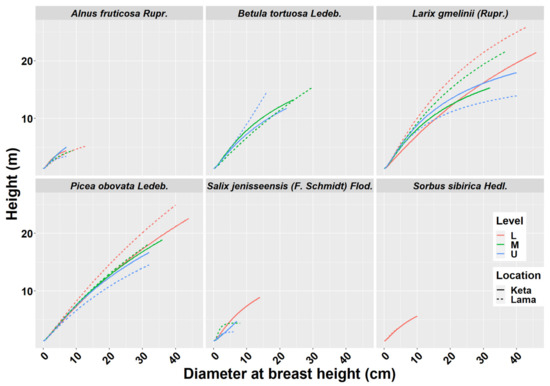
Figure 1.
Height-diameter models of six tree species at two locations of Keta and Lama. Statistical parameters of models are presented in Table 1. Level—L—lower elevational zone, M—middle elevational zone, U—upper elevational zone.

Table 1.
Statistical parameters of derived height-diameter models (Model—identification number of the derived model, PAR—coefficient in Equation (1), COEF—value of the coefficient in Equation (1), SE—standard error, t value—t-value of Student test of a coefficient, p value—probability of t-value and its significance as follows: .—90%, *—95%, **—99%, ***—99.9%, R2—R-squared; Level: elevational zone L—Lower, M—Middle, U—Upper, Number—number of trees).
2.2. Crown Radius—Height Models
Crown width has an important role in many biomass models. From the obtained data we derived 29 models describing the relationship of crown radius to tree height at the individual location and elevational category (Figure 2). The results revealed a lower impact of the elevational gradient than the one found for height-diameter models. In the case of Alnus fruticosa Rupr., the statistical test did not confirm significant differences between the elevational zones at the Keta location (Figure A2). At the Lama location, we found a significant difference between the upper and the middle zones, as well as between the upper and the lower zones. The relationship between the crown radius and tree height in the lower and middle zones of Lama has a linear pattern. The relationships in the upper zone are non-linear and similar at both locations. The models of individual locations significantly differed from each other (Figure A2).
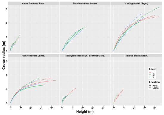
Figure 2.
Crown radius—height models of six tree species at two locations of Keta and Lama. Statistical parameters of models are presented in Table 2. Level: L—lower elevational zone, M—middle elevational zone, U—upper elevational zone.
The models derived for Betula tortuosa Ledeb. at Keta significantly differed between the elevational zones, while at Lama we did not reveal such an influence of elevation. Moreover, the models derived for locations were significantly different. In the case of Larix gmelinii (Rupr.), we did not reveal any significant differences between the models of individual elevational zones, but we confirmed significant differences between the locations. The models for Picea obovata Ledeb. significantly differed between the elevational zones at Keta, while the lowest crown radii were found in the middle elevational zone, and the largest ones in the lower zone. At Lama, the significant difference was found between the models for the lower and the middle zones, which were characterised by the lowest and the largest crown radii, respectively. The models significantly differed between locations. For Salix jenisseensis (F. Schmidt) Flod. we did not find significant differences between elevational zones at Keta. At Lama we could derive only one model for the middle elevational zone. The models for individual locations were not significantly different. For Sorbus sibirica Hedl. we created only three models in total, one for the lower elevational zone at Keta, and the other two for two elevational zones at Lama, which did not differ from each other significantly. However, the models for Keta and Lama were significantly different. Parameters of crown radius-height models for individual tree species, elevational zones, and locations are presented in Table 2. In general, the models explained from 58% to 99% of crown radius variability depending on the tree species, location, and elevational zone (Table 2).
Table 2.
Statistical parameters of derived crown radius-height models (Model—identification number of the derived model, PAR—coefficient in Equation (2), COEF—value of the coefficient in Equation (2), SE—standard error, t value—t-value of Student’s test of coefficient, p value—probability of t value and its significance as follows: .—90%, *—95%, **—99%, ***—99.9%, R2—R-squared; Level: elevational zone L—Lower, M—Middle, U—Upper, Number—number of trees).
2.3. Above-Ground Biomass (AGB)
The biomass of tree species was calculated using regional allometric equations derived by [38,43,44] for thick and thin trees separately. In general, biomass production decreases with elevation. We found this pattern at Lama, where the aboveground biomass of all tree species decreased from 90 t/ha to 26 t/ha, i.e., by 3.5 times along the elevational gradient covering 300 m. At Keta, the decreasing trend was recorded only up to middle elevations (206 m a.s.l.). At higher elevations, biomass stock increased and reached the value of about 77 t/ha at the highest elevation. The aboveground biomass of thin trees (DBH ≤ 7 cm) was slightly increasing with the elevation at Lama, while at Keta we found a substantial decreasing trend (Figure 3).
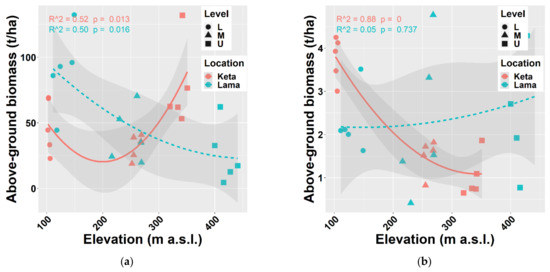
Figure 3.
Relationship between elevation and aboveground living biomass (a) of all trees together, (b) of thin trees (with a height of at least 0.1 m up to DBH ≤ 7 cm) at two locations. Points represent biomass values at individual sample plots. Lines represent fitted non-linear models, and grey areas show 95% confidence intervals around the fitted models. Level: L—lower elevational zone, M—middle elevational zone, U—upper elevational zone.
The analysis of individual tree species revealed that the aboveground biomass of Alnus fruticosa Rupr. decreased with elevation at both locations. In contrast, the aboveground tree biomass of Betula tortuosa Ledeb. increased with elevation at either of the studied locations. In the case of Salix jenisseensis (F. Schmidt) Flod. and Sorbus sibirica Hedl. we observed a decrease in aboveground biomass with elevation at Keta, while at Lama we did not find any strong trend with elevation, and the aboveground biomass remained unchanged. The relationship between the elevation and the biomass of the main tree species Larix gmelinii (Rupr.) and Picea obovata Ledeb. resembles the general pattern of all tree species together (compare Figure 3 and Figure 4).
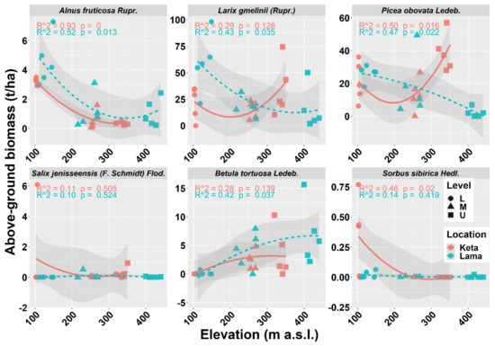
Figure 4.
Relationship between elevation and aboveground living tree biomass of individual tree species at two locations. Points represent biomass values at individual sample plots. Lines represent fitted non-linear models, and grey areas show 95% confidence intervals around the fitted models. Level: L—lower elevational zone, M—middle elevational zone, U—upper elevational zone.
Next, we looked at the relationship between elevation and deadwood biomass that included both fine and coarse woody debris (stumps, standing dead trees, snags, logs, and buried deadwood) (Figure 5a) and the total biomass, i.e., living and dead together (Figure 5b). The revealed trends are similar to the one of the aboveground living biomass of all tree species or main tree species presented above. Total deadwood biomass at individual sample plots varied between 0.06 t/ha and 21.45 t/ha, while the recorded total biomass stock was from 6.47 t/ha to 149 t/ha.
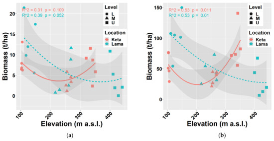
Figure 5.
Relationships between elevation and biomass of deadwood (a) and total biomass (living and deadwood together) (b) at two locations. Points represent biomass values at individual sample plots. Lines represent fitted non-linear models, and grey areas show 95% confidence intervals around the fitted models. Level: L—lower elevational zone, M—middle elevational zone, U—upper elevational zone.
2.4. Relationships of Selected Site Characteristics to Biomass of Tree Species
We performed a univariate correlation and regression analysis to examine the relationship of 99 environmental variables (see Figure A5, and Materials and Methods for more details) to the total biomass of tree species (living and dead together) in investigated locations. In total, we found 10 significant relationships at 95% significance level (Figure A5). Only one of them (biomass versus amount of K in mg/kg in the upper soil layer up to 10 cm depth) was significant at 99% significance level (R2 = 0.44). Out of 10 significant correlations, six were negative and four positive ones. The total biomass was significantly positively correlated with terrain types (represented in models as dummy variables), where water inflow exceeds water outflow from a site, such as a slope base, a bottom of the slope, a terrace gutter, and a slope basin. Positive relationships were also revealed between biomass and K and Mn content in the upper soil layer up to 10 cm, and the C:N ratio in the soil layer in the depth of 20–30 cm. Negative relationships were revealed between the biomass and the terrain type, where water outflow prevails, e.g., a summit, or an upper part of a slope. The decrease in biomass was also found with the increase in d15N, Al-d, Al-o in the upper soil layer (0–10 cm), and the proportion of hygroscopic water in the second and third soil layers (10–20 or 20–30 cm).
When analysing the relationships of site characteristics to total biomass (living and dead together) for individual locations separately, no significant correlation was revealed at Keta. On the contrary, 28 significant relationships (Figure A5) were found at Lama, where the elevational gradient was more pronounced in previous analyses. Seven of them were positive and the remaining 21 were negative. R2 of significant relationships fluctuated between 0.27 and 0.72. The highest correlation was found between total biomass and K content in the first soil layer (0–10 cm) (Figure 6).
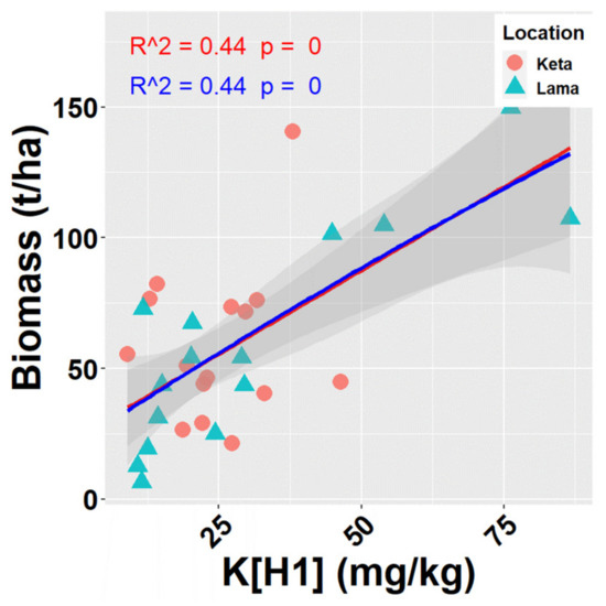
Figure 6.
Relationships of K content in soil in depth 0–10 cm (K[H1] (mg/kg)) to total biomass of tree species (aboveground living + deadwood). Points represent values at individual sample plots. Lines represent fitted models (red—linear, blue—quadratic), and grey areas show 95% confidence intervals around the fitted models.
The analysis of the impact of site characteristics on the aboveground biomass of living trees revealed similar results for the total biomass. The analysis regardless of location found 6 characteristics significantly affecting aboveground living biomass, while for Keta no significant correlation was revealed, and for Lama 27 significant relationships were detected.
Multiple regression analyses of all data together regardless of location partially confirmed results of the univariate correlation analysis (Figure 7). Considering the existing data structure, a multiple regression model can include 28 variables at maximum. Most frequently included variables were elevation and the two terrain types mentioned above. These were followed by soil characteristics, namely d15N in the third soil layer, and C:N ratios in the third and the second soil layers, i.e., in depths of 20–30, and 10–20 cm, respectively. The next commonly included variable was K content in the first soil layer, which was found to be the most highly correlated variable to biomass in univariate analyses. Further variables represented site characteristics (forms of micro-relief and humus, and slope), and other soil characteristics (content of sand, hygroscopic water, content of chemical elements Mn, Ca, and of oxalate- and dithionite-extractable Al). Statistical parameters of multiple models (Figure 7) indicated that the optimal multivariate model should include 12 to 14 predictors (Cp). Models with this number of independent variables can explain 87 to 91% of biomass variability. The model with 13 predictors including an intercept is presented in Table 3. The results show that all included variables were significant, and their multicollinearity did not exceed recommended thresholds, i.e., their values of the variance inflation factor was below 10 [45,46,47]. The types of terrain were the most influential variables in the model (Table 3).
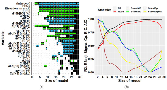
Figure 7.
Predictors (a) and statistical characteristics (b) of multiple regression models of tree biomass derived for both locations together. Size of model represents the number of predictors included in the multiple regression model. Participation of individual variables in multiple regression models of biomass is indicated in the left figure by black squares, while black dots indicate their absence. Green dots inside black squares indicate significant positive impacts of respective variables, while blue dots represent their significant negative impacts. Predictors are identified by a combination of variable abbreviations, soil layers, and units if applicable as follows: Variables: Al-d—content of dithionite-extractable aluminium in (mg/kg), Al-o—content of oxalate-extractable aluminium in (mg/kg), C—carbon content in (%), C:N—C:N ratio, Ca—calcium content in (mg/kg), d15N—ratio of stable nitrogen isotopes 15N:14N in (‰), Elevation—elevation in (m a.s.l.), FRFS—form of relief—foot of slope, FRUS—form of relief—peak, upper slope, HW—hygroscopic water in (%), K—potassium content in (mg/kg), Mn—manganese content in (mg/kg), Moder—humus form, Mor—humus form, MR`-^`—micro relief (flat terrain along the contour line and concave terrain along the slope), MR`-v`—micro relief (flat terrain along the contour line and convex terrain along the slope), N—nitrogen content in (%), SA—sand fraction in (%), SD—slope downward in (°), SU—slope upward (°); soil layers presented in square brackets: H1—layer at 0–10 cm soil depth, H2—10–20 cm depth, H3—20–30 cm depth; statistical characteristics of derived models presented in figure (b) are as follows: R2—R-squared, R2adj—adjusted R-squared, AIC—AKAIKE information criterion, BIC—BAYESIAN information criterion, Cp—Mallows’ statistic, Sigma—residual standard deviation.
Table 3.
Overview of variables included in the optimal multiple regression model (Biomass = f(Variable1,…, Variable13)) derived for Keta and Lama together and their statistical characteristics (H1—layer 0–10 cm, H2—layer 10–20 cm, H3—layer 20–30 cm, MR`-^`—Micro relief—`-^`, HW (%)—hygroscopic water, SA (%)—sand fraction, C:N—C:N ratio, C (%)—carbon content, d15N (‰)—ratio of stable nitrogen isotopes 15N:14N, Elevation (m a.s.l.)—elevation, FRUS—form of relief (peak, upper slope), FRFS—form of relief(foot of slope), SD (°)—slope downward, Estimate = regression coefficient for the respective variable, SE= standard error, t value—t-value of Student test of coefficient, p value—probability of t value and its significance of p value as follows: *—95%, **—99%, ***—99.9%, VIF—variance inflation factor, Fdf—degrees of freedom, Fp—p value for F, R2adj—adjusted R-squared).
When deriving multiple regressions for individual locations we could include only 14 predictors at maximum due to a smaller amount of available data. Most of the variables selected as predictors were soil characteristics. The optimal model for Keta (Figure 8) contained 4 to 6 independent variables (including an intercept). The models of these dimensions explained 46–62% of biomass variability. The most significant variables were latitude, C:N ratio in different soil layers, forms of micro-relief (plain along the contour line, concave along the slope). The 5-dimensional model also included the fraction of clay in 10–20 cm soil depth (Table 4).
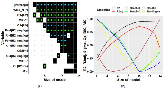
Figure 8.
Predictors (a) and statistical characteristics (b) of multiple regression models of tree biomass derived for Keta location. Size of model represents the number of predictors included in the multiple regression model. Participation of individual variables in multiple regression models of biomass is indicated in the left figure by black squares, while black dots indicate their absence. Green dots inside black squares indicate significant positive impacts of respective variables, while blue dots represent their significant negative impacts. Predictors are identified by a combination of variable abbreviations, soil layers, and units if applicable as follows: Variables: Al-d—content of dithionite-extractable aluminium in (mg/kg), Al-o—content of oxalate-extractable aluminium in (mg/kg), C:N—C:N ratio, CL—clay fraction in (%), Fe-d—content of dithionite-extractable iron in (mg/kg), Fe-o—content of oxalate-extractable iron in (mg/kg), MR`^-`—micro relief (concave terrain along the contour line and flat terrain along the slope), MR`-^`—Micro relief (flat terrain along the contour line and concave terrain along the slope), WGS_N—latitude in (°); soil layers presented in square brackets: H1—layer at 0–10 cm soil depth, H2—10–20 cm depth, H3—20–30 cm depth; statistical characteristics of derived models presented in figure (b) are as follows: R2—R-squared, R2adj—adjusted R-squared, AIC—Akaike information criterion, BIC—Bayesian information criterion, Cp—Mallows’ statistic, Sigma—residual standard deviation.
Table 4.
Overview of variables included in the optimal multiple regression model (Biomass = f(Variable1, …, Variable5)) derived for Keta and their statistical characteristics (H1—soil layer 0–10 cm, H2—layer 10–20 cm, H3—layer 20–30 cm, C:N—C:N ratio, WGS_N (°)—latitude, CL (%)—clay fraction, Estimate—regression coefficient for the respective variable, SE—standard error, t value—t-value of Student test of coefficient, p value—probability of t value and its significance of p value as follows: .—90%,*—95%, **—99%, ***—99.9%, VIF—variance inflation factor, Fdf—degrees of freedom, Fp— p value for F, R2adj—adjusted R-squared).
The optimal multiple model for Lama contained 7 variables (Figure 9) and explained 85% of biomass variability (Table 5). The most frequently included variable was K content in soil depth of 0–10 cm. The content of nitrogen isotope d15N in the top (0–10 cm) and bottom (20–30 cm) soil layers were other frequent significant characteristic in multiple models. The other variables were latitude, thickness of O horizon, and the fraction of sand in 0–10 cm soil depth.
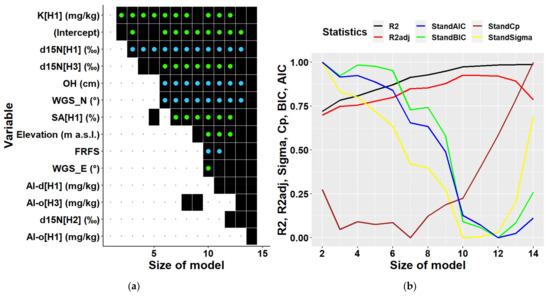
Figure 9.
Predictors (a) and statistical characteristics (b) of multiple regression models of tree biomass derived for Lama location. Size of model represents the number of predictors included in the multiple regression model. Participation of individual variables in multiple regression models of biomass is indicated by black squares, while black dots indicate their absence. Green dots inside black squares indicate significant positive impacts of respective variables, while blue dots represent their significant negative impacts. Predictors are identified by a combination of variable abbreviations, soil layers, and units if applicable as follows: Variables: Al-d—content of dithionite-extractable aluminium in (mg/kg), Al-o—content of oxalate-extractable aluminium in (mg/kg), d15N—ratio of stable nitrogen isotopes 15N:14N in ‰, Elevation—elevation in (m a.s.l.), FRFS—form of relief (foot of slope), K—potassium content in (mg/kg), OH—thickness of O horizon—surface organic layer in (cm), SA—sand fraction in (%), WGS_E—longitude in (°), WGS_N—latitude in (°). Soil layers presented in square brackets: H1—layer at 0–10 cm soil depth, H2—10–20 cm depth, H3—20–30 cm depth. Statistical characteristics of derived models presented in figure (b) are as follows: R2—R-squared, R2adj—adjusted R-squared, AIC—Akaike information criterion, BIC—Bayesian information criterion, Cp—Mallows’ statistic, Sigma—residual standard deviation.
Table 5.
Overview of variables included in the optimal multiple regression model (Biomass = f(Variable1, …, Variable7)) derived for Lama and their statistical characteristics (H1—soil layer 0–10 cm, H2—layer 10–20 cm, H3—layer 20–30 cm, d15N (‰)—ratio of stable nitrogen isotopes 15N:14N, K (mg/kg)—potassium content, WGS_N (°)—latitude, OH (cm)—thickness of O horizon—surface organic layer, SA (%)—sand fraction, Estimate = regression coefficient for the respective variable, SE= standard error, t value—t-value of Student test of coefficient, p value—probability of t value and its significance of p value as follows: .—90%, *—95%, **—99%, ***—99.9%, VIF—variance inflation factor, Fdf—degrees of freedom, Fp—p value for F, R2adj—adjusted R-squared).
3. Discussion
Height-diameter models are useful tools for the estimation of tree heights from their diameters as well as for the evaluation of site productivity [11,13,14,15]. A number of different equations have been used to describe the relationship between diameter and height. We used a model by [48,49], because this function was able to describe the relationship between the tree diameter and height of thin trees. The suitability of the specific equation depends on environmental conditions [12]. For example, [17] found that the Chapman–Richards function was best able to describe their empirical data for Dahurian larch, while [16] revealed that the most suitable function changed between the ecoregions of the Daxing’an Mountains Region. Our results also showed differences between locations and elevational zones, although not all of them were significant (Figure A2). However, for each tree species we found some significant differences either between locations or elevational zones or both.
Similar results were revealed for species-specific crown radius-height models that explained around 90% of variability in crown radius data (Table 2). The models differed between the locations for each tree species except for Salix (Figure A4). The impact of the elevational gradient on this relationship was most profound for Picea obovata Ledeb. followed by Alnus fruticosa Rupr. (Figure A4). The crown width is a useful characteristic in studies dealing with tree competition, stand density, spacing and stocking relationships, wildlife habitat suitability models, as well as production [50]. In the past, the relationship of the crown radius to stem diameter was usually studied. The analyses showed that this relationship can be accurately described with a linear model [50,51,52]. However, nowadays remote sensing techniques are becoming the more commonly used approaches of data acquisition. Hence, the relationships to tree height, which is one of the most easily determined variables using remote sensing methods [53], may be of a greater value. The authors of [54] showed that the information about crown diameter explained 78% of the biomass variance. Other works have also supported the use of crown parameters in biomass estimation [19,55,56].
In our study, we applied regional allometric equations derived by [38,43,44] that included crown diameter as one predictor of aboveground tree biomass of thin trees. The equations applied to thick trees used DBH or a combination of DBH and height as predictors. These variables are known to provide reasonably accurate species- and region-specific biomass predictions [23,28,57]. Although diameter based allometric models are most commonly used, adding a tree height into the model usually increases the accuracy of biomass predictions [23,58,59,60]. Biomass amounts estimated in our study were comparable with quantities presented in previous works from the area around the Lama lake at similar elevations, latitudes, and longitudes [39,40,41]. However, while the cited works focused on the upper timber line, we analysed tree species biomass along the elevational gradient starting almost at the lake water level. In addition, our study contains new information on species-specific dimensions, biomass, and biomass components (living and dead), and thus enhances the knowledge about forest ecosystems of the region. Previous works from the area around the Lama lake [39,40,41] documented the most pronounced upward shift of the upper timber line on southern slopes (111 ± 74 m).
Our analysis revealed a significant reduction in aboveground biomass with the increasing elevation at the Lama location, which is consistent with the results of [39,41,61]. However, at the Keta location, the relationship of biomass to elevation did not have a decreasing trend but followed a U shape (Figure 3). This may be the result of the opposing impacts of elevation and micro-site conditions [62]. Topographic factors (elevation, slope, and aspect) have a significant impact on AGB (carbon) [63,64,65]. The authors of [39] confirmed a strong influence of aspect in the region of our interest, and our data showed that the aspects of the two locations differed from each other. Plots at Lama were situated on slopes with the E and SE aspect, while south was the prevailing aspect of Keta plots, followed by the western and the northern ones. Inversed impacts are known to occur around large lakes due to moisture [66] that can substantially change at a regional level because of the terrain morphology [67]. At Lama we found several significant correlations of tree biomass with site characteristics that represent either soil conditions or terrain morphology (Figure A5). Strong impacts of relief forms on forest cover were revealed by [68].
From soil characteristics, potassium content in the upper soil layer was found to be closely related to the amount of tree biomass. A high amount of potassium in soil favours the aboveground biomass production [69]. The importance of K for plant functioning was reported by, e.g., [70]. Potassium affects the stomata opening, photosynthesis, enzyme activation, and protein synthesis [71,72]. However, the relationship between tree biomass and potassium content in soil is bidirectional. On one side, a tree obtains potassium from soil. On the other hand, foliage biomass is the main source of K in soil [73]. Hence, the cycle of potassium in forest ecosystems is semi-closed. Unlike other base cations, the distribution and seasonal dynamics of K in forest ecosystems is strongly affected by biotic processes [74] because it is most prone to leaching [75]. Further fate of the leached K is driven by soil hydrologic conditions, its absorptive ability, soil microorganisms and plant roots [75]. Potassium reabsorption by plants may be higher at sites with lower percolation, i.e., where the humus layer is thicker and soil water movement caused by temperature is lower. Timber harvest, fire, land use changes, and nitrogen deposition also influence the biotic availability of potassium [76].
At Lama, two highly significant negative correlations of tree biomass to site characteristics were revealed (Figure 9). The first one was with the d15N isotope abundance in the upper soil layer (0–10 cm). The natural nitrogen stable isotope (15N) has been used in studies of N cycling in an ecosystem because its abundance is the result of a number of biogeochemical processes [77]. Nitrogen isotopes provide insights about the forms of nitrogen sources, and the processes N has been involved in [78]. Our analysis revealed higher abundances of d15N at plots with less tree biomass occurring at higher elevations. This corresponds with the knowledge that soil and plant d15N are positively correlated with mean annual temperature and negatively correlated with mean annual precipitation total [77], or the fact that in many wet or cold ecosystems d15N values in foliage and soil are depleted [79]. In multiple regression models derived for Lama, the abundance of d15N isotope in the bottom soil layer 20–30 cm was a significant predictor of tree biomass occurring in all models with three or more independent variables (Figure 9). Unlike its abundance in the first layer, the d15N abundance in the bottom layer showed a positive association with biomass in the derived models including the 7-dimensional model for Lama (Table 5). This is probably because organic matter containing N in deeper soil layers originated from trees and their roots, possibly also older and more humified than the organic matter in the topsoil (upper 10 cm), originating from shrubs that are more abundant under an open forest canopy.
Another highly significant correlation at Lama was found between the biomass and content of oxalate-extractable aluminium in the first soil layer (Figure A5). Aluminium is known for its toxicity to plants, especially if present in large amounts in acidic soils [80,81]. Measured soil pH at our locations indicated that soils were slightly to moderately acidic, while a lower pH was observed at Lama. Acidification of the location can be caused by acid rain containing emissions of Norilsk metallurgical Combine [61]. Our univariate correlation analysis revealed a negative impact of oxalate-extractable aluminium on tree biomass at Lama (Figure A5). Multiple regressions contained two other predictors representing aluminium in different soil layers, too. We found the opposing impacts of oxalate-extractable and dithionite-extractable aluminium in derived models for Lama, Keta and for both locations together (Figure 7, Figure 8 and Figure 9). In joint models, dithionite-extractable aluminium in the first soil layer, which is an indicator of more advanced weathering, had a significant positive impact on biomass. This is consistent with the study of [80] which revealed that at low concentrations aluminium can influence growth positively. The influence of aluminium oxides (dithionite and oxalate extractions) bears a witness to more intense soil weathering accompanied by a lower pH, and thus increased availability of the sorption capacity for soil organic carbon (organic matter) that in turn increases the soil capacity for nutrients.
Other highly significant variables affecting tree biomass at Lama were latitude (negative impact) and longitude (positive impact) that occurred also in multiple regression models derived for Lama (see Figure 9), while in the case of Keta only latitude was among multiple predictors (Figure 8), and in models derived for both locations together they did not occur at all (Figure 7). Although their influence is well-known and documented [82], revealing significant correlations at a micro-spatial level indicates substantial changes in site conditions even at such a small scale. Side slopes of the Putorana table mountain are steep, and the valleys are deep. At bottom parts, soils are deeper and have enough water, due to which biomass production is high there. Ecosystem productivity is also affected by soil organic matter, the stable fraction of which is humus [83]. Mor forms of humus and the thickness of O horizon were significantly positively corelated to the tree biomass at Lama, while moder forms had a negative correlation to tree biomass (Figure 7). In multiple regression models for Lama, only the thickness of the O horizon was included as a predictor, and its impact was negative indicating interrelationships between independent variables (Figure 9, Table 5). On the contrary, the models for Keta and for both locations together contained humus forms, but not the thickness of O horizon.
Soil texture has a profound influence on forest growth because it affects soil water-holding and ion exchange capacity, retention of organic matter, and aeration [71,72]. At Lama, the sand content in the first soil layer (0–10 cm) had a significant impact on tree biomass in univariate and multiple regression models (Figure A5 and Figure 9). It was also one of predictors in models derived for both locations together (Figure 7). However, while its impact at Lama was positive, in general models it was negative (Table 3 and Table 5). At Lama, more sand was found in soils at the bottom of the elevational gradient, where stands were most productive. The relationships of biomass at Lama to the content of clay, silt or hygroscopic water were negative, but the variables were not included in location-specific multiple regression models. These results reflect the more intense weathering at the upper parts of the elevational gradient because (1) the O horizon is thinner at the mountain top, due to which soil can be warmed up faster than in the bottom parts characterised by thicker layers of O horizon thermally insulating soil, (2) of strong thermal inversion along the slopes next to the lakes [66]. Models for Keta contained only clay content in the middle soil layer (10–20 cm) as a predictor (Figure 8). The percentage of hygroscopic water in the first and the third layers occurred in models for both locations, while their impact changed with model dimensions (Figure 7). Negative univariate correlations between biomass and hygroscopic water indicate that the more soil water is bound to soil particles and thus unavailable to plants [84], the less biomass is produced. In addition, the presence of hygroscopic water in soil indicates the presence of allophane or imogolite, which may limit phosphorus availability. The interrelationships are complex, some may support and some limit the growth, as shown in some of the derived multiple models, where the trend was reversed, which was documented by higher values of VIF for the parameters.
Although the C:N ratio in soil is an important characteristic of ecosystems because it affects nitrogen cycling and the process of decomposition [85] and is considered as an indicator of site quality [86], it was included only in multiple models for Keta or both locations together (Figure 7, Figure 8 and Figure 9). The univariate correlation analysis revealed that C:N ratios in all soil layers had a positive impact on tree biomass (Figure A5). However, when the variables were included in multiple regression models, only the impact of C:N ratio in the second layer remained positive, while the partial influence of the other two was negative (Figure 7 and Figure 8, Table 3 and Table 4). A similar situation was observed for the content of oxalate-extractable and dithionite-extractable iron. These variables occurred only in models derived for Keta, in which the content of dithionite-extractable iron in the second layer had a positive association, while oxalate-extractable iron in the same soil layer had a negative relationship with tree biomass (Figure 8), although the univariate regression analysis found positive correlations of both of them to tree biomass (Figure A5). Previous research showed that the shortage of Fe in soil can have a negative effect on biomass production [87], which is not the case in the analysed areas.
4. Materials and Methods
4.1. Empirical Data
Data used for the analysis come from field measurements performed in the western part of Putorana Plateau (Figure 10) in the area around the Lama and Keta lakes (Krasnoyarsk region, Russia) in the years 2018 and 2019. This part of northern Russia is one of the least accessible and least studied regions. The mountain range represents the biggest monolithic mountain range of the Russian Arctic, which is almost completely located north of the arctic circle [39,61] extending from 89° to 101° E and from 67° to 71° N. The geological substrate is the tholeiitic basalt characterised by homogeneous chemical and mineralogical composition with high contents of Al2O3 and Fe2O3 [88]. With respect to the geological and geomorphological features, it is a flat-topped basalt crystalline massif (plateau) with elevations averaging 900–1200 m and reaching a maximum of 1701 m a.s.l. in the central part (Kamen Mountain). Multiple uplifts on the Putorana Plateau have generated deep radial tectonic fractures in this area in the form of narrow gorges and canyons with the trappean structure of slopes [39,41,68]. The Putorana Plateau is in the subarctic climate belt, at the boundary between the Atlantic and Siberian regions, in the continuous permafrost zone. The climate is excessively continental [88], and the amount of precipitation is significantly higher than anywhere else in the north of Eastern Siberia. The cold subarctic climate sustains the presence of continuous permafrost table at 1 to 3 m soil depth and a widespread development of cryogenic processes, e.g., solifluction [89].
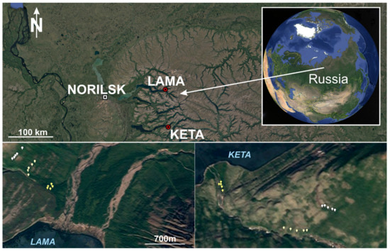
Figure 10.
Location of sample plots in Russia, at Lama and Keta lakes (Krasnoyarsk region).
The unique geological formation of Putorana Plateau was the main reason for assigning this region to the World Natural Heritage in 2010 [90]. The area is characterised by the occurrence of unique natural complexes with high biodiversity and the presence of intrazonal communities of flora and fauna. The upper timberline is formed by Dahurian larch (Larix gmelinii Rupr.) and lies in the interval of 200 to 900 m a.s.l., depending on regional and local habitat conditions.
At each location we gathered data along an elevational gradient divided into three elevational zones. In every elevational zone we established five circular sample plots, each of 500 m2 situated along the same contour line. Hence, in total we established 30 sample plots. More than 150 characteristics describing site, terrain, soil, ecological, and tree species-specific features, were assessed in the field at each plot. The tree species was defined as a species of a tree shape with a potential tree height of 5 m or more. Plot position and elevation were measured with a GPS tool Garmin 60CSx. Aspect and slope were measured in degrees and were determined with a compass and Hypsometer Haglöf Vertex, respectively. Relief forms were specified visually based on the plot position along the slope and with regard to the prevailing water movement (predominant water inflow, outflow, or balanced). We identified five forms of relief: flat terrain, peak/upper slope, middle slope, foot of slope, and indistinct. Micro-relief was evaluated based on the terrain curvature along the contour line and along the slope using three basic terrain shapes: - flat land, ^ concave terrain, v convex terrain. Hence, 9 possible combinations were identified in total, e.g., -^ is flat land along the contour line and concave terrain along the slope. Then, we assessed the form of humus, estimated moisture conditions (dry, optimal, wet sites), relative coverage of aboveground rocks, and of fine woody debris (%). Mean diameter of fine woody debris, diameter, and length of coarse woody debris (CWD) pieces were measured. Each CWD piece was assigned into one of four decay classes (1—recently dead wood with intact bark, present twigs and branches, round shape, smooth surface, intact texture, and the position elevated on support points, 2—solid wood with present bark and twigs with diameter over 1 cm, 3—moderately soft wood, twigs absent, bark mostly absent, 4—very soft deadwood with no bark, twigs or branches, strongly fragmented, in contact with the ground along the whole length). In total, we gathered information about 240 pieces of deadwood. In the case of living trees, we collected information about individual tree species for four categories: trees with diameter at breast height (DBH) above 7 cm, trees with tree height exceeding 1.3 m and DBH below 7 cm, trees with a height from 0.2 to 1.3 m, and trees smaller than 0.2 m). For each category we determined tree species cover, number of trees, mean tree height, mean crown radius, and minimum, maximum, and mean diameter at breast height where applicable. In total, we measured 576 trees with tree height exceeding 1.3 m. The crown radius was measured at 382 trees representing all above-listed size categories. The basic description of sample plots sites is presented in Table 6, while the basic characteristics of individual tree species are shown in Table 7.
Table 6.
Basic characteristics of sample plots. Mean annual temperature (MAT) and mean annual precipitation total (MAP) were calculated from the Version 4 of the CRU TS Monthly High-Resolution Gridded Multivariate Climate Dataset [91].
Table 7.
Basic characteristics of tree species.
4.2. Soil Sampling and Analyses
Soil sampling was performed at each research plot, i.e., 30 soil pits were excavated to the depth of 0.3–0.4 m from the mineral soil surface in total. Three soil samples, each weighing approximately 150 g, were taken from 0.1 m, 0.2 m, and 0.3 m depths at each plot. The soil texture was determined by the pipette method after the removal of organic compounds with hydrogen peroxide (H2O2) and clay dispersion [92]. The soil pH was measured in a deionized water suspension of air-dried soil at a soil-to-solution ratio of 1:2.5 by Testo 206 pH1 instrument (Testo SE & Co. KGaA, Lenzkirch, Germany). Contents of C and N in the fine earth (<2 mm) were obtained through dry combustion method using CN analyser (Vario Isotope Cube, Elementar Analysis Systems GmbH, Hanau, Germany). The C:N ratio was calculated as an indicator of POM presence (>10), as opposed to minerally associated organic matter (<13) [93]. Free Fe (Fe-o, Fe-d) and Al (Al-o, Al-d) contained in the fine earth fraction were extracted using 0.2 M ammonium oxalate and sodium dithionite-citrate solutes [94]. Dithionite-citrate extraction represents both crystalline and poorly crystalline Fe oxides [95,96]. The value of Al d is thus believed to represent the amount of Al substituted in Fe oxides and hydroxides [97], whereby Al substitution in iron oxides indicates stronger weathering conditions [98]. Oxalate-extractable Fe, Al, and Si represent poorly crystalline aluminosilicates, ferrihydrite, and Al and Fe in organic complexes [95,96]. Barium chloride (BaCl2), 0.1 M, was used to extract exchangeable Ca, Mg, and K [94]. Free Fe, Al, and exchangeable cations concentrations were measured by inductively coupled plasma—optical emission spectrometer (ICP—OES Agilent 5100, USA).
4.3. Statistical Analyses
Standard statistical approaches were applied (univariate and multivariate correlation and regression analyses, ANOVA) to perform the analyses using the available tools in R environment [99]. We used the nls function in R to derive non-linear height-diameter and crown radius-height models. For multiple analyses we used the lmSubsets function [100], and the ggplot2 package to visualise the results [101].
4.4. Non-Linear Height-Diameter Models and Crown Radius-Height Models of Trees
Tree height (h) is the second most important variable after the diameter at breast height (DBH) because it describes a vertical stand structure and serves as a good indicator of site productivity [102]. The relationship between tree diameter and tree height is related to the growth stage, i.e., its position and shape changes with stand age. This is caused by varying growth rates of height and diameter in individual developmental stages of stands. The height curve of natural forests is usually in a balanced state, i.e., its position and shape do not change. Literature sources present a number of functions suitable for modelling the relationship between tree height and diameter [15,48,49,103,104,105,106,107,108]. In our study we applied a slightly modified Prodan function [48,49] in the following form:
where h is tree height in m, DBH is tree diameter in cm, a and b are regression coefficients.
Tree crown size is another important parameter that affects tree growth, carbon sequestration, shading, filtering of fine air particulates, and risk of windbreaking [52]. The majority of allometric relationships between crown diameter, radius, or crown projection use tree diameter as a predictor. However, currently, remote sensing techniques have become to be more frequently used. Therefore, we decided to take a tree height as an explanatory variable since height can be directly obtained from remote sensing data. Moreover, such a relationship can be also applied to trees that did not reach a height of 1.3 m yet. To describe the relationship between the crown radius (CR) and tree height (h) we used the following nonlinear equation:
where CR is crown radius in m, h is tree height in m, a and b are regression coefficients.
4.5. Quantifying the Above-Ground Biomass (AGB)
Biomass plays an important role in biogeochemical cycles, ecosystem functioning, and the formation of community structure [57]. For the quantification of the biomass of individual tree species recorded in our study we used previously published models for the total aboveground biomass of living trees including stem, branches, twigs, and foliage, from similar geographical regions [38,43,44]. The aboveground biomass of trees with DBH above 7 cm was calculated using DBH as a sole predictor (Picea), or using both DBH and height (Larix, Betula, Alnus, Salix, Sorbus). In the case of smaller trees that did not reach DBH of 7 cm or a height of 1.3 m, we calculated the aboveground biomass as a function of tree height and crown diameter.
The biomass amount of deadwood was calculated for individual components: aboveground coarse deadwood, buried deadwood, standing dead trees, snags, stumps, fine woody debris. First, the volume of deadwood was determined as follows. The volume of aboveground deadwood and buried deadwood pieces was calculated using Huber formula based on their middle stem diameter and length [102,109]. The volume of standing dead trees or snags was quantified using the standard volume equation with DBH, height, and a taper factor [110] as independent variables, while the taper factor was set to 0.4 [102]. The volume of stumps was calculated as a volume of a cylinder using its diameter and height. The volume of fine woody debris was derived from its cover area and mean diameter. In the next step, volume was converted to biomass using wood density. We set the mean wood density of living trees to 400 kg/m3 and reduced it with regard to decay stage following the work of [111]. Hence, the density of wood in decay stage 1, 2, 3, and 4 represented 90%, 75%, 50%, and 35% of the living wood density, respectively. In the case of buried deadwood it was only 20%.
5. Conclusions
The presented study brings new information and knowledge about tree vegetation from a part of northern Russia that is one of the least accessible and least studied regions. This study is the first one focusing on the area around Keta lake. The developed local height-diameter and crown radius-height models for six tree species (Larix gmelinii (Rupr.), Picea obovata Ledeb., Alnus fruticosa Rupr., Salix jenisseensis (F. Schmidt) Flod., Betula tortuosa Ledeb., Sorbus sibirica Hedl.) were site and elevation-specific, and explained most of the variability in studied relationships. They may help to improve estimates of biomass and carbon stock in the studied regions in the future. The total tree biomass stock including aboveground tree biomass and aboveground and buried deadwood varied between 6.47 t/ha and 149 t/ha, while the total deadwood biomass fluctuated from 0.06 to 21.45 t/ha. The general pattern of decreasing biomass production with elevation was observed at Lama. At the Keta location, the relationship of biomass to elevation followed a U shape. This may be the result of the opposing impacts of elevation and micro-site conditions.
Terrain morphology and soil conditions had a significant impact on tree biomass. The most influential predictors in multiple regression models for both locations together were the form of relief representing the peak, and upper slope, followed by elevation, the form of relief representing the foot of slope, ratio of stable nitrogen isotopes 15N:14N in soil depth of 20–30 cm, and C:N ratio in soil depth of 10–20 cm. However, the multiple models derived for individual locations separately differed in most of predictors they contained. Hence, the results indicate that microsite environmental conditions have a substantial effect on tree biomass in the studied locations. Further detailed research is needed to thoroughly understand the functioning and dynamics in this part of the world.
Author Contributions
Conceptualization, J.M.; methodology, J.M., V.P., E.G. and K.M.; formal analysis, J.M. and K.M.; investigation, J.M., V.P., E.G., P.F. and M.H.; data curation, J.M. and E.G.; writing—original draft preparation, J.M. and K.M.; writing—review and editing: J.M., K.M., V.P. and E.G..; supervision, V.P.; project administration, V.P.; funding acquisition, V.P. All authors have read and agreed to the published version of the manuscript.
Funding
This research was funded by the Slovak Research and Development Agency of the Slovak Republic, Project No. APVV-17-0676.
Institutional Review Board Statement
Not applicable.
Informed Consent Statement
Not applicable.
Data Availability Statement
The data presented in this study are available on request from the corresponding author. The data are not publicly available due to the ongoing analyses.
Acknowledgments
The organisational, logistical support and help from Konstantin Prosekin and Alexander Matasov are gratefully acknowledged.
Conflicts of Interest
The authors declare no conflict of interest.
Abbreviations
WGS_N—latitude, WGS_E—longitude, Elevation—elevation, SU—slope upward, SD—slope downward, SR—surface rockiness, OH—thickness of O horizon—surface organic layer, FRUS—form of relief (peak, upper slope), FRMS—form of relief (middle slope), FRFS—form of relief (foot of slope), Aspect—E, Aspect—N—, Aspect—NW—, Aspect—S—, Aspect—SE—, Aspect—SW—, Moder—humus, Moder—form, Mor—humus form, SMN—soil moisture normal, SMW—soil moisture wet, MR`--`, `-^`, `-v`, `^-`, `^^`, `^v`, `v^`—micro relief (combinations of terrain curvature along the contour line and along the slope using three basic terrain shapes: - flat land, ^ concave terrain, v convex terrain), H1—soil layer 0–10 cm, H2—layer 10–20 cm, H3—layer 20–30 cm, N—nitrogen content, C—carbon content, C:N—C:N ratio, d13N—ratio of stable carbon isotopes 13C:12C, d15N—ratio of stable nitrogen isotopes 15N:14N, pH[H2O]—power of hydrogen in soil, HW—hygroscopic water, SA—sand fraction, SI—silt fraction, CL—clay fraction, P—phosphorus content, Al-d—content of dithionite-extractable aluminium, Fe-d—content of dithionite-extractable iron, Mn-d—content of dithionite-extractable manganese, Al-o—content of oxalate-extractable aluminium, Fe-o—content of oxalate-extractable iron, Mn-o—content of oxalate-extractable manganese, Ca—calcium content, K—potassium content, Mg—magnesium content, Na—sodium content, Al—aluminium content, Fe—iron content, Mn—manganese content.
Appendix A
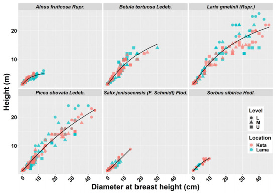
Figure A1.
General height-diameter models for six tree species at two locations of Keta and Lama. Statistical parameters of models are presented in Table 1. Level: L—lower elevational zone, M—middle elevational zone, U—upper elevational zone.
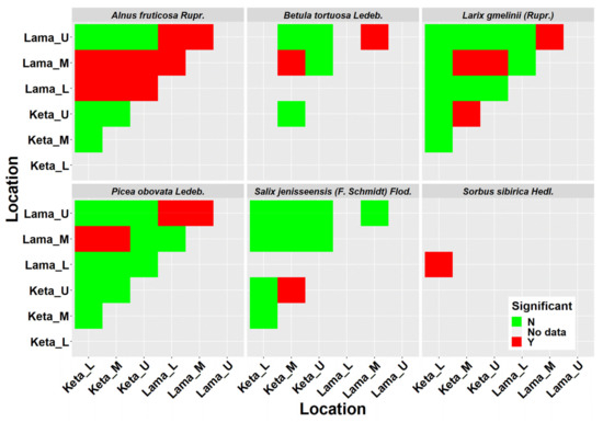
Figure A2.
ANOVA-based statistical comparison of derived height-diameter models (Table 1). N means not significant, Y means significant at 95% significance level. L, M, U represent lower, middle, and upper elevational zones, respectively.
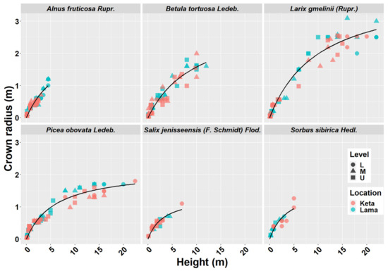
Figure A3.
General crown radius, height models for six tree species at two locations of Keta and Lama. Statistical parameters of models are presented in Table 2. Level: L—lower elevational zone, M—middle elevational zone, U—upper elevational zone.
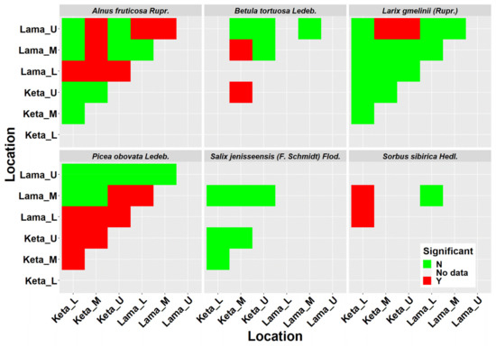
Figure A4.
ANOVA-based statistical comparison of derived crown radius-height models (Table 2). N means not significant, Y means significant at 95% significance level. L, M, U represent lower, middle, and upper elevational zones, respectively.
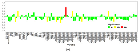
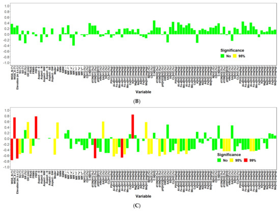
Figure A5.
Correlation analysis of site characteristics with tree biomass (living + dead) for both locations (Keta, Lama) together (A), Keta (B) and Lama (C).
References
- Frelich, L.E. Boreal and Taiga Biome. In Encyclopedia of the World’s Biomes; Goldstein, M.I., DellaSala, D.A., Eds.; Elsevier: Oxford, UK, 2020; pp. 103–115. ISBN 978-0-12-816097-8. [Google Scholar]
- Flade, L.; Hopkinson, C.; Chasmer, L. Allometric Equations for Shrub and Short-Stature Tree Aboveground Biomass within Boreal Ecosystems of Northwestern Canada. Forests 2020, 11, 1207. [Google Scholar] [CrossRef]
- Kajimoto, T.; Matsuura, Y.; Osawa, A.; Abaimov, A.P.; Zyryanova, O.A.; Isaev, A.P.; Yefremov, D.P.; Mori, S.; Koike, T. Size–Mass Allometry and Biomass Allocation of Two Larch Species Growing on the Continuous Permafrost Region in Siberia. For. Ecol. Manag. 2006, 222, 314–325. [Google Scholar] [CrossRef]
- Liu, M.; Liu, G.; Gong, L.; Wang, D.; Sun, J. Relationships of Biomass with Environmental Factors in the Grassland Area of Hulunbuir, China. PLoS ONE 2014, 9, e102344. [Google Scholar] [CrossRef] [PubMed] [Green Version]
- Yang, Y.; Dou, Y.; An, S. Environmental Driving Factors Affecting Plant Biomass in Natural Grassland in the Loess Plateau, China. Ecol. Indic. 2017, 82, 250–259. [Google Scholar] [CrossRef]
- Dong, L.-H.; Zhang, L.; Li, F. Additive Biomass Equations Based on Different Dendrometric Variables for Two Dominant Species (Larix Gmelini Rupr. and Betula Platyphylla Suk.) in Natural Forests in the Eastern Daxing’an Mountains, Northeast China. Forests 2018, 9, 261. [Google Scholar] [CrossRef] [Green Version]
- Alonzo, M.; Andersen, H.-E.; Morton, D.C.; Cook, B.D. Quantifying Boreal Forest Structure and Composition Using UAV Structure from Motion. Forests 2018, 9, 119. [Google Scholar] [CrossRef] [Green Version]
- Gauthier, S.; Bernier, P.; Kuuluvainen, T.; Shvidenko, A.Z.; Schepaschenko, D.G. Boreal Forest Health and Global Change. Science 2015, 349, 819–822. [Google Scholar] [CrossRef]
- Botkin, D.B.; Simpson, L.G. Biomass of the North American Boreal Forest: A Step toward Accurate Global Measures. Biogeochemistry 1990, 9, 161–174. [Google Scholar]
- Neigh, C.S.; Nelson, R.F.; Ranson, K.J.; Margolis, H.; Montesano, P.M.; Sun, G.; Kharuk, V.; Naesset, E.; Wulder, M.A.; Anderson, H. LiDAR-Based Biomass Estimates, Boreal Forest Biome, Eurasia, 2005–2006; ORNL DAAC: Oak Ridge, TN, USA, 2015. [CrossRef]
- Huang, S.; Price, D.; Titus, J.S. Development of Ecoregion-Based Height–Diameter Models for White Spruce in Boreal Forests. For. Ecol. Manag. 2000, 129, 125–141. [Google Scholar] [CrossRef]
- Sharma, M. Comparing Height-Diameter Relationships of Boreal Tree Species Grown in Plantations and Natural Stands. For. Sci. 2016, 62, 70–77. [Google Scholar] [CrossRef]
- Stout, B.B.; Shumway, D.L. Site Quality Estimation Using Height and Diameter. For. Sci. 1982, 28, 639–645. [Google Scholar] [CrossRef]
- Vanclay, J.K. Modelling Forest Growth and Yield: Applications to Mixed Tropical Forests; CAB International: Wallingford, UK, 1994; ISBN 978-0-85198-913-6. [Google Scholar]
- Wykoff, W.; Crookston, N.; Stage, A. User’s Guide to the Stand Prognosis Model; U.S. Department of Agriculture, Forest Service, Intermountain Forest and Range Experiment Station: Ogde, UT, USA, 1982; p. 112.
- Dai, Z.-D.; Jiang, L.-C. Ecoregion Based Height-Diameter Models for Larix Gmelinii Rupr. in Daxingan Mountains. Bull. Bot. Res. 2015, 35, 583. [Google Scholar] [CrossRef]
- Enzinga, G.Y.; Jiang, L.-C. Evaluation of Region and Subregion-Based Heightdiameter Models for Dahurian Larch (Larix Gmelinii) in Daxing’an Mountains in China. Appl. Ecol. Env. Res. 2019, 17, 13567. [Google Scholar] [CrossRef]
- Ravindranath, N.H.; Ostwald, M. Methods for Estimating Above-Ground Biomass. In Carbon Inventory Methods Handbook for Greenhouse Gas Inventory, Carbon Mitigation and Roundwood Production Projects; Advances in Global Change Research; Springer: Dordrecht, The Netherlands, 2008; pp. 113–147. ISBN 978-1-4020-6547-7. [Google Scholar]
- Wilkes, P.; Disney, M.; Vicari, M.B.; Calders, K.; Burt, A. Estimating Urban above Ground Biomass with Multi-Scale LiDAR. Carbon Balance Manag. 2018, 13, 10. [Google Scholar] [CrossRef] [PubMed]
- Forrester, D.I.; Tachauer, I.H.H.; Annighoefer, P.; Barbeito, I.; Pretzsch, H.; Ruiz-Peinado, R.; Stark, H.; Vacchiano, G.; Zlatanov, T.; Chakraborty, T.; et al. Generalized Biomass and Leaf Area Allometric Equations for European Tree Species Incorporating Stand Structure, Tree Age and Climate. For. Ecol. Manag. 2017, 396, 160–175. [Google Scholar] [CrossRef]
- Eggleston, S.; Buendia, L.; Miwa, K.; Ngara, T.; Tanabe, K. IPCC Guidelines for National Greenhouse Gas Inventories; Institute for Global Environmental Strategies: Hayama, Japan, 2006. [Google Scholar]
- Dong, L.; Zhang, L.; Li, F. A Compatible System of Biomass Equations for Three Conifer Species in Northeast, China. For. Ecol. Manag. 2014, 329, 306–317. [Google Scholar] [CrossRef]
- Wang, C. Biomass Allometric Equations for 10 Co-Occurring Tree Species in Chinese Temperate Forests. For. Ecol. Manag. 2006, 222, 9–16. [Google Scholar] [CrossRef]
- Wang, X.; Bi, H.; Ximenes, F.; Ramos, J.; Li, Y. Product and Residue Biomass Equations for Individual Trees in Rotation Age Pinus Radiata Stands under Three Thinning Regimes in New South Wales, Australia. Forests 2017, 8, 439. [Google Scholar] [CrossRef] [Green Version]
- Ali, A.; Xu, M.-S.; Zhao, Y.-T.; Zhang, Q.-Q.; Zhou, L.-L.; Yang, X.-D.; Yan, E.-R. Allometric Biomass Equations for Shrub and Small Tree Species in Subtropical China. Silva Fenn. 2015, 49, 1275. [Google Scholar] [CrossRef] [Green Version]
- Brown, S.; Gillespie, A.J.R.; Lugo, A.E. Biomass Estimation Methods for Tropical Forests with Applications to Forest Inventory Data. For. Sci. 1989, 35, 881–902. [Google Scholar] [CrossRef]
- Berner, L.T.; Alexander, H.D.; Loranty, M.M.; Ganzlin, P.; Mack, M.C.; Davydov, S.P.; Goetz, S.J. Biomass Allometry for Alder, Dwarf Birch, and Willow in Boreal Forest and Tundra Ecosystems of Far Northeastern Siberia and North-Central Alaska. For. Ecol. Manag. 2015, 337, 110–118. [Google Scholar] [CrossRef]
- He, A.; McDermid, G.J.; Rahman, M.M.; Strack, M.; Saraswati, S.; Xu, B. Developing Allometric Equations for Estimating Shrub Biomass in a Boreal Fen. Forests 2018, 9, 569. [Google Scholar] [CrossRef] [Green Version]
- Konôpka, B.; Pajtík, J.; Šebeň, V.; Surový, P.; Merganičová, K. Woody and Foliage Biomass, Foliage Traits and Growth Efficiency in Young Trees of Four Broadleaved Tree Species in a Temperate Forest. Plants 2021, 10, 2155. [Google Scholar] [CrossRef] [PubMed]
- Konôpka, B.; Pajtík, J.; Šebeň, V.; Surový, P.; Merganičová, K. Biomass Allocation into Woody Parts and Foliage in Young Common Aspen (Populus tremula L.)—Trees and a Stand-Level Study in the Western Carpathians. Forests 2020, 11, 464. [Google Scholar] [CrossRef] [Green Version]
- Smith, W.B.; Brand, G.J. Allometric Biomass Equations for 98 Species of Herbs, Shrubs, and Small Trees; Research Note NC-299; U.S. Deptartment of Agriculture, Forest Service, North Central Forest Experiment Station: St. Paul, MN, USA,, 1983; p. 299. [CrossRef]
- Chaturvedi, R.K.; Raghubanshi, A.S. Aboveground Biomass Estimation of Small Diameter Woody Species of Tropical Dry Forest. New For. 2013, 44, 509–519. [Google Scholar] [CrossRef]
- Chave, J.; Réjou-Méchain, M.; Búrquez, A.; Chidumayo, E.; Colgan, M.S.; Delitti, W.B.C.; Duque, A.; Eid, T.; Fearnside, P.M.; Goodman, R.C.; et al. Improved Allometric Models to Estimate the Aboveground Biomass of Tropical Trees. Glob. Chang. Biol. 2014, 20, 3177–3190. [Google Scholar] [CrossRef] [PubMed]
- Huff, S.; Ritchie, M.; Temesgen, H. Allometric Equations for Estimating Aboveground Biomass for Common Shrubs in Northeastern California. For. Ecol. Manag. 2017, 398, 48–63. [Google Scholar] [CrossRef]
- Pajtík, J.; Konôpka, B.; Šebeň, V. Mathematical Biomass Models for Young Individuals of Forest Tree Species in the Region of the Western Carpathians; National Forest Centre, Forest Research Institut: Zvolen, Slovakia, 2018; ISBN 978-80-8093-241-1.
- Liu, Z.; Chen, R.; Song, Y.; Han, C.; Yang, Y. Estimation of Aboveground Biomass for Alpine Shrubs in the Upper Reaches of the Heihe River Basin, Northwestern China. Environ. Earth Sci. 2015, 73, 5513–5521. [Google Scholar] [CrossRef]
- Huang, C.; Feng, C.; Ma, Y.; Liu, H.; Wang, Z.; Yang, S.; Wang, W.; Fu, S.; Chen, H.Y.H. Allometric Models for Aboveground Biomass of Six Common Subtropical Shrubs and Small Trees. Res. Sq. 2021, 1–14. [Google Scholar] [CrossRef]
- Usoltsev, A.V.; Chasovskikh, V.P.; Noritsina, Y.V.; Noritsin, D.V. Allometric Models of Tree Biomass for Airborne Laser Scanning and Ground Inventory of Carbon Pool in the Forests of Eurasia: Comparative Analysis. Sib. J. For. Sci. 2016, 68–76. [Google Scholar]
- Grigoriev, A.A.; Дэви, Н.М.; Кукарских, В.В.; Вьюхин, С.О.; Галимова, А.А.; Моисеев, П.А.; Φомин, В.В. Структура и динамика древостоев верxней грaницы леса в западной части плато Путорана (Structure and dynamics of the stands of the upper forest boundary in the western part of the Putorana plateau). Экoлoгия 2019, 4, 243–254. [Google Scholar] [CrossRef]
- Im, S.T.; Charuk, V.I. КЛИМАТИЧЕСКИ ИНДУЦИРОВАННЫЕ ИЗМЕНЕНИЯ В ЭКОТОНЕ АЛЬПИЙСКОЙ ЛЕСОТУНДРЫ ПЛАТО ПУТОРАНА (Use of Space-Based Earth Information Climate-Induced Changes in the Ecotone of the Alpine Forest Tundra Putorana Plateau). Исследование Земли Космоса 2013, 5, 32–44. [Google Scholar]
- Kirdyanov, A.V.; Hagedorn, F.; Knorre, A.A.; Fedotova, E.V.; Vaganov, E.A.; Naurzbaev, M.M.; Moiseev, P.A.; Rigling, A. 20th Century Tree-Line Advance and Vegetation Changes along an Altitudinal Transect in the Putorana Mountains, Northern Siberia. Boreas 2012, 41, 56–67. [Google Scholar] [CrossRef]
- Farjon, A. A Handbook of the World’s Conifers (2 Vols.); Brill: Leiden, The Netherlands, 2010; Volume 1, ISBN 90-04-17718-3. [Google Scholar]
- Usoltsev, A.V.; Kolchin, K.V.; Azarenok, V.A. On Possibilities for Application of Generic and Regional Allometric Models When Estimating Spruce Tree Biomass. Agrar. Bull. Ural. 2017, 160, 33–37. [Google Scholar]
- Usoltsev, A.V.; Gavrilin, D.S.; Malenko, A.A.; Semyshev, M.M. Tree Biomass of Larix Sibirica and Larix Gmelinii: Comparative Analysis. Bull. Altai State Agric. Univ. 2013, 12, 57–61. [Google Scholar]
- Hair, J.F., Jr.; Anderson, R.E.; Tatham, R.L.; Black, W.C. Multivariate Data Analysis, 3rd ed.; Macmillan: New York, NY, USA, 1995. [Google Scholar]
- Kutner, M.; Nachtsheim, C.; Neter, J.; Li, W. Applied Linear Statistical Models with Student CD; McGraw-Hill Education: New York, NY, USA, 2004; ISBN 978-0-07-310874-2. [Google Scholar]
- O’brien, R.M. A Caution Regarding Rules of Thumb for Variance Inflation Factors. Qual. Quant. 2007, 41, 673–690. [Google Scholar] [CrossRef]
- Curtis, R.O. Height-Diameter and Height-Diameter-Age Equations For Second-Growth Douglas-Fir. For. Sci. 1967, 13, 365–375. [Google Scholar] [CrossRef]
- Prodan, M. Forest Biometrics; Pergamon Press: New York, NY, USA, 1968. [Google Scholar]
- Lockhart, B.R.; Weih, R.C.; Smith, K.M. Crown Radius and Diameter at Breast Height Relationships for Six Bottomland Hardwood Species. J. Ark. Acad. Sci. 2005, 59, 110–115. [Google Scholar]
- Gill, S.; Biging, G.; Murphy, E. Modeling Conifer Tree Crown Radius and Estimating Canopy Cover. For. Ecol. Manag. 2000, 126, 405–416. [Google Scholar] [CrossRef] [Green Version]
- Pretzsch, H.; Biber, P.; Uhl, E.; Dahlhausen, J.; Rötzer, T.; Caldentey, J.; Koike, T.; van Con, T.; Chavanne, A.; Seifert, T.; et al. Crown Size and Growing Space Requirement of Common Tree Species in Urban Centres, Parks, and Forests. Urban For. Urban Green. 2015, 14, 466–479. [Google Scholar] [CrossRef] [Green Version]
- Ganz, S.; Käber, Y.; Adler, P. Measuring Tree Height with Remote Sensing—A Comparison of Photogrammetric and LiDAR Data with Different Field Measurements. Forests 2019, 10, 694. [Google Scholar] [CrossRef] [Green Version]
- Popescu, S.C.; Wynne, R.H.; Nelson, R.F. Measuring Individual Tree Crown Diameter with Lidar and Assessing Its Influence on Estimating Forest Volume and Biomass. Can. J. Remote Sens. 2003, 29, 564–577. [Google Scholar] [CrossRef]
- Goodman, R.C.; Phillips, O.L.; Baker, T.R. The Importance of Crown Dimensions to Improve Tropical Tree Biomass Estimates. Ecol. Appl. 2014, 24, 680–698. [Google Scholar] [CrossRef] [PubMed] [Green Version]
- Soenen, S.A.; Peddle, D.R.; Hall, R.J.; Coburn, C.A.; Hall, F.G. Estimating Aboveground Forest Biomass from Canopy Reflectance Model Inversion in Mountainous Terrain. Remote Sens. Environ. 2010, 114, 1325–1337. [Google Scholar] [CrossRef]
- Altanzagas, B.; Luo, Y.; Altansukh, B.; Dorjsuren, C.; Fang, J.; Hu, H. Allometric Equations for Estimating the Above-Ground Biomass of Five Forest Tree Species in Khangai, Mongolia. Forests 2019, 10, 661. [Google Scholar] [CrossRef] [Green Version]
- Bi, H.; Turner, J.; Lambert, M.J. Additive Biomass Equations for Native Eucalypt Forest Trees of Temperate Australia. Trees 2004, 18, 467–479. [Google Scholar] [CrossRef]
- Dong, L.; Zhang, L.; Li, F. Developing Additive Systems of Biomass Equations for Nine Hardwood Species in Northeast China. Trees 2015, 29, 1149–1163. [Google Scholar] [CrossRef]
- Li, H.; Zhao, P. Improving the Accuracy of Tree-Level Aboveground Biomass Equations with Height Classification at a Large Regional Scale. For. Ecol. Manag. 2013, 289, 153–163. [Google Scholar] [CrossRef]
- Matveev, S.; Gupalov, D. Silvicultural and Dendroclimatic Analysis of Plantations Gmelin Larch Western Part of the Putoran Plateau. For. Eng. J. 2015, 5, 54–65. [Google Scholar] [CrossRef]
- Körner, C. The Use of ‘Altitude’ in Ecological Research. Trends Ecol. Evol. 2007, 22, 569–574. [Google Scholar] [CrossRef]
- Du, Q.; Xu, J.; Wang, J.; Zhang, F.; Ji, B. Correlation between Forest Carbon Distribution and Terrain Elements of Altitude and Slope. J. Zhejiang A&F Univ. 2013, 30, 330. [Google Scholar]
- Fan, Y.; Zhou, G.; Shi, Y.; Du, H.; Zhou, Y.; Xu, X. Effects of terrain on stand structure and vegetation carbon storage of Phyllostachys edulis forest. Sci. Silvae Sin. 2013, 49, 177–182. [Google Scholar]
- Shen, A.; Wu, C.; Jiang, B.; Deng, J.; Yuan, W.; Wang, K.; He, S.; Zhu, E.; Lin, Y.; Wu, C. Spatiotemporal Variations of Aboveground Biomass under Different Terrain Conditions. Forests 2018, 9, 778. [Google Scholar] [CrossRef] [Green Version]
- Malyshev, L. Levels of the Upper Forest Boundary in Northern Asia. Vegetatio 1993, 109, 175–186. [Google Scholar] [CrossRef]
- Zan, B.; Yu, Y.; Dong, L.; Li, J.; Zhao, G.; Zhang, T. Numerical Study of the Impact of Complex Terrain and Soil Moisture on Convective Initiation. Atmosphere 2020, 11, 871. [Google Scholar] [CrossRef]
- Abaimov, A.P.; Zyryanova, O.A.; Mikhaylova, I.A.; Moroz, S.N.; Shitova, S.A. Multipurpose Mapping of the Forests of the Central Putorana Upland, East Siberia. Mapp. Sci. Remote Sens. 1995, 32, 274–283. [Google Scholar] [CrossRef]
- Epron, D.; Laclau, J.-P.; Almeida, J.C.R.; Goncalves, J.L.M.; Ponton, S.; Sette, C.R.; Delgado-Rojas, J.S.; Bouillet, J.-P.; Nouvellon, Y. Do Changes in Carbon Allocation Account for the Growth Response to Potassium and Sodium Applications in Tropical Eucalyptus Plantations? Tree Physiol. 2011, 32, 667–679. [Google Scholar] [CrossRef] [PubMed] [Green Version]
- Tripler, C.E.; Kaushal, S.S.; Likens, G.E.; Todd Walter, M. Patterns in Potassium Dynamics in Forest Ecosystems. Ecol. Lett. 2006, 9, 451–466. [Google Scholar] [CrossRef] [PubMed]
- Binkley, D.; Fisher, R.F. Ecology and Management of Forest Soils; Wiley: New York, NY, USA, 2019; ISBN 978-1-119-45565-3. [Google Scholar]
- Marschner, H. Mineral Nutrition of Higher Plants; Elsevier Science: San Diego, CA, USA, 1995; ISBN 978-0-08-057187-4. [Google Scholar]
- Pokrovsky, O.S.; Viers, J.; Dupré, B.; Chabaux, F.; Gaillardet, J.; Audry, S.; Prokushkin, A.S.; Shirokova, L.S.; Kirpotin, S.N.; Lapitsky, S.A.; et al. Biogeochemistry of Carbon, Major and Trace Elements in Watersheds of Northern Eurasia Drained to the Arctic Ocean: The Change of Fluxes, Sources and Mechanisms under the Climate Warming Prospective. Comptes Rendus Geosci. 2012, 344, 663–677. [Google Scholar] [CrossRef]
- Vitousek, P. Nutrient Cycling and Limitation; Molina, M.J., Morel, F.M.M., Morgan, J.J., Tilman, D., Eds.; Princeton University Press: Princeton, NJ, USA, 2004. [Google Scholar]
- Moore, T.R. Winter-Time Litter Decomposition in a Subarctic Woodland. Arct. Alp. Res. 1983, 15, 413–418. [Google Scholar] [CrossRef]
- Bock, M.D.; Van Rees, K.C. Forest Harvesting Impacts on Soil Properties and Vegetation Communities in the Northwest Territories. Can. J. For. Res. 2002, 32, 713–724. [Google Scholar] [CrossRef]
- Sheng, W.; Yu, G.; Fang, H.; Liu, Y.; Wang, Q.; Chen, Z.; Zhang, L. Regional Patterns of 15N Natural Abundance in Forest Ecosystems along a Large Transect in Eastern China. Sci. Rep. 2015, 4, 4249. [Google Scholar] [CrossRef] [Green Version]
- Hyodo, F.; Kusaka, S.; Wardle, D.A.; Nilsson, M.-C. Changes in Stable Nitrogen and Carbon Isotope Ratios of Plants and Soil across a Boreal Forest Fire Chronosequence. Plant Soil 2013, 367, 111–119. [Google Scholar] [CrossRef]
- Handley, L.; Austin, A.; Robinson, D.; Scrimgeour, C.; Raven, J.; Heaton, T.; Schmidt, S.; Stewart, G. The 15N Natural Abundance (D15N) of Ecosystem Samples Reflects Measures of Water Availability. Aust. J. Plant Physiol. 1999, 26, 185–199. [Google Scholar] [CrossRef]
- Kidd, P.S.; Proctor, J. Effects of Aluminium on the Growth and Mineral Composition of Betula Pendula Roth. J. Exp. Bot. 2000, 51, 1057–1066. [Google Scholar] [CrossRef] [Green Version]
- Rahman, M.A.; Lee, S.-H.; Ji, H.C.; Kabir, A.H.; Jones, C.S.; Lee, K.-W. Importance of Mineral Nutrition for Mitigating Aluminum Toxicity in Plants on Acidic Soils: Current Status and Opportunities. Int. J. Mol. Sci. 2018, 19, 3073. [Google Scholar] [CrossRef] [Green Version]
- Zhang, H.; Wang, K.; Xu, X.; Song, T.; Xu, Y.; Zeng, F. Biogeographical Patterns of Biomass Allocation in Leaves, Stems and Roots in China’s Forests. Sci. Rep. 2015, 5, 15997. [Google Scholar] [CrossRef] [Green Version]
- Osman, K.T. Organic Matter of Forest Soils. In Forest Soils: Properties and Management; Osman, K.T., Ed.; Springer International Publishing: Cham, Switzerland, 2013; pp. 63–76. ISBN 978-3-319-02541-4. [Google Scholar]
- Kozlowski, T.T. Soil Moisture and Absorption of Water by Tree Roots. J. Arboric. 1987, 13, 39–46. [Google Scholar]
- Stall, C.; Fuller, R.; Mihuc, T.; Jones, J.; Woodcock, T. Nitrogen Cycling and Dynamics in Upland Managed and Preserved Watersheds of the Adirondack Mountains, New York. Sci. Discipulorum 2008, 3, 1–10. [Google Scholar]
- Yamakura, T.; Sahunalu, P. Soil Carbon/Nitrogen Ratio as a Site Quality Index for Some South-East Asian Forests. J. Trop. Ecol. 1990, 6, 371–377. [Google Scholar] [CrossRef]
- Hellal, F.A.; Amer, A.K.; Zaghloul, A.M. Effect of Applied Iron on Iron Desorption in Soil and Uptake by Wheat Plants. J. Appl. Biol. Sci. 2008, 2, 79–86. [Google Scholar]
- Krivolutskaya, N.A.; Kedrovskaya, T.B. Structure and Composition of the Nadayansky Lava Flow: An Example of the Homogeneity of Lava Flows of the Siberian Trap Province. Geochem. Int. 2020, 58, 363–376. [Google Scholar] [CrossRef]
- Shahgedanova, M. The Physical Geography of Northern Eurasia; Oxford Regional Environments; Oxford University Press: Oxford, UK, 2003; ISBN 978-0-19-823384-8. [Google Scholar]
- Butorin, A.A.; Maksakovskiy, N.V.; Trofimova, E.V. Landforms as a Pivotal Component of the World Natural Heritage Sites: Case Studies in Russia. Int. J. Conserv. Sci. 2021, 12, 205–216. [Google Scholar]
- Harris, I.; Osborn, T.J.; Jones, P.; Lister, D. Version 4 of the CRU TS Monthly High-Resolution Gridded Multivariate Climate Dataset. Sci. Data 2020, 7, 109. [Google Scholar] [CrossRef] [Green Version]
- Blume, H.P.; Stahr, K.; Leinweber, P. Bodenkundliches Praktikum: Eine Einführung in Pedologisches Arbeiten Für Ökologen, Land- Und Forstwirte, Geo- Und Umweltwissenschaftler; Springer: Berlin/Heidelberg, Germany, 2011; ISBN 978-3-8274-2733-5. [Google Scholar]
- Lavallee, J.M.; Soong, J.L.; Cotrufo, M.F. Conceptualizing Soil Organic Matter into Particulate and Mineral-Associated Forms to Address Global Change in the 21st Century. Glob. Chang. Biol. 2020, 26, 261–273. [Google Scholar] [CrossRef] [Green Version]
- Extractable Al, Fe, Mn, and Si. In Soil Sampling and Methods of Analysis; Carter, M.R.; Gregorich, E.G. (Eds.) CRC Press: Boca Raton, FL, USA, 2007; ISBN 978-0-429-12622-2. [Google Scholar]
- Cornell, R.M.; Schwertmann, U. The Iron Oxides: Structure, Properties, Reactions, Occurrences and Uses; Wiley: New York, NY, USA, 2006; ISBN 978-3-527-60644-3. [Google Scholar]
- Mikutta, R.; Kleber, M.; Torn, M.S.; Jahn, R. Stabilization of Soil Organic Matter: Association with Minerals or Chemical Recalcitrance? Biogeochemistry 2006, 77, 25–56. [Google Scholar] [CrossRef]
- Kaufhold, S.; Ufer, K.; Kaufhold, A.; Stucki, J.W.; Anastácio, A.S.; Jahn, R.; Dohrmann, R. Quantification of Allophane from Ecuador. Clays Clay Miner. 2010, 58, 707–716. [Google Scholar] [CrossRef]
- Fitzpatrick, R.W.; Schwertmann, U. Al-Substituted Goethite—An Indicator of Pedogenic and Other Weathering Environments in South Africa. Geoderma 1982, 27, 335–347. [Google Scholar] [CrossRef]
- R Core Team. R: A Language and Environment for Statistical Computing; Foundation for Statistical Computing: Vienna, Austria, 2019. [Google Scholar]
- Hofmann, M.; Gatu, C.; Kontoghiorghes, E.J.; Colubi, A.; Zeileis, A. LmSubsets: Exact Variable-Subset Selection in Linear Regression. J. Stat. Softw. 2020, 93, 1–21. [Google Scholar] [CrossRef]
- Wickham, H. Ggplot2: Elegant Graphics for Data Analysis; Springer-Verlag: New York, NY, USA, 2016; ISBN 978-3-319-24277-4. [Google Scholar]
- Šmelko, Š. Dendrometria; Vydavateľstvo TU Zvolen: Zvolen, Slovakia, 2007. [Google Scholar]
- Levakovic, A. Analytical Form of Growth Laws. Glas. Za Sumske Pokuse 1935, 4, 189–282. [Google Scholar]
- Loetsch, F.; Zohrer, F.; Haller, K.E. Forest Inventory; BLV Verlagsgesellschaft: Munchen, Germany, 1973; ISBN 3405111269. [Google Scholar]
- Michailoff, I. Zahlenmäßiges Verfahren Für Die Ausführung Der Bestandeshöhenkurven. Cbl. Thar. Forstl. Jahrb. 1943, 6, 273–279. [Google Scholar]
- Näslund, M. Functions and Tables for Computing the Cubic Volume of Standing Trees. Pine, Spruce and Birch in Southern Sweden and in the Whole of Sweden. Rep. For. Res. Inst. Swed. 1947, 36, 68. [Google Scholar]
- Ratkowsky, D.A.; Giles, D.E.A. Handbook of Nonlinear Regression Models; Statistics Series; M. Dekker: New York, NY, USA, 1990; ISBN 978-0-8247-8189-7. [Google Scholar]
- Zeide, B. Accuracy of Equations Describing Diameter Growth. Can. J. For. Res. 1989, 19, 1283–1286. [Google Scholar] [CrossRef]
- West, P.W. Tree and Forest Measurement, 3rd ed.; Springer International Publishing: Cham, Switzerland, 2015; ISBN 978-3-319-14707-9. [Google Scholar]
- Van Laar, A.; Akça, A. Forest Mensuration, 2nd ed.; Managing Forest Ecosystems; Springer: Dordrecht, The Netherlands, 2007; ISBN 978-1-4020-5990-2. [Google Scholar]
- Merganičová, K.; Merganič, J. Coarse Woody Debris Carbon Stocks in Natural Spruce Forests of Babia Hora. J. For. Sci. 2010, 56, 397–405. [Google Scholar] [CrossRef] [Green Version]
Publisher’s Note: MDPI stays neutral with regard to jurisdictional claims in published maps and institutional affiliations. |
© 2021 by the authors. Licensee MDPI, Basel, Switzerland. This article is an open access article distributed under the terms and conditions of the Creative Commons Attribution (CC BY) license (https://creativecommons.org/licenses/by/4.0/).