Sharp Feature Detection as a Useful Tool in Smart Manufacturing

Abstract

Industry 4.0 comprises a wide spectrum of developmental processes within the management of manufacturing and chain production. Presently, there is a huge effort to automate manufacturing and have automatic control of the production. This intention leads to the increased need for high-quality methods for digitization and object reconstruction, especially in the area of reverse engineering. Commonly used scanning software based on well-known algorithms can correctly process smooth objects. Nevertheless, they are usually not applicable for complex-shaped models with sharp features. The number of the points on the edges is extremely limited due to the principle of laser scanning and sometimes also low scanning resolution. Therefore, a correct edge reconstruction problem occurs. The same problem appears in many other laser scanning applications, i.e., in the representation of the buildings from airborne laser scans for 3D city models. We focus on a method for preservation and reconstruction of sharp features. We provide a detailed description of all three key steps: point cloud segmentation, edge detection, and correct B-spline edge representation. The feature detection algorithm is based on the conventional region-growing method and we derive the optimal input value of curvature threshold using logarithmic least square regression. Subsequent edge representation stands on the iterative algorithm of B-spline approximation where we compute the weighted asymmetric error using the golden ratio. The series of examples indicates that our method gives better or comparable results to other methods.

1. Introduction

Industry 4.0 is the trend towards automation and data exchange in manufacturing technologies and processes. Industry 4.0 factories have machines which are augmented with wireless connectivity and sensors, connected to a system that can visualize the entire production line and make decisions on its own. Smart manufacturing is a broad category of manufacturing that employs computer-integrated manufacturing, high levels of adaptability and rapid design changes, digital information technology, and more flexible technical workforce training [1,2].

Our work covers the part of automation in manufacturing and reverse engineering for design changes. The widespread availability of cheap commercial depth sensors or multi-camera setups leads to their common usage in manufacturing engineering, especially in rapid product development [3]. Therefore, the point cloud has become the regular type of the representation used e.g., in reverse engineering (RE) and rapid prototyping (RP). The precision, scanning speed and variety of processing algorithms create suitable conditions for its common usage.

A key problem in the RE/RP integration, as mentioned in [4], is the transformation of a set of dense points obtained in the RE process to a fitting model that can be used. In Figure 1, the reverse engineering process is described.

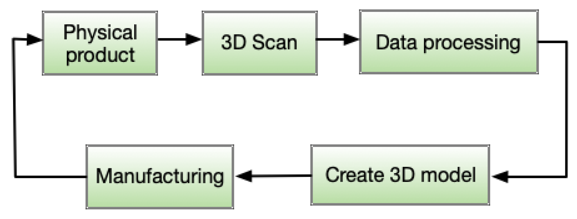
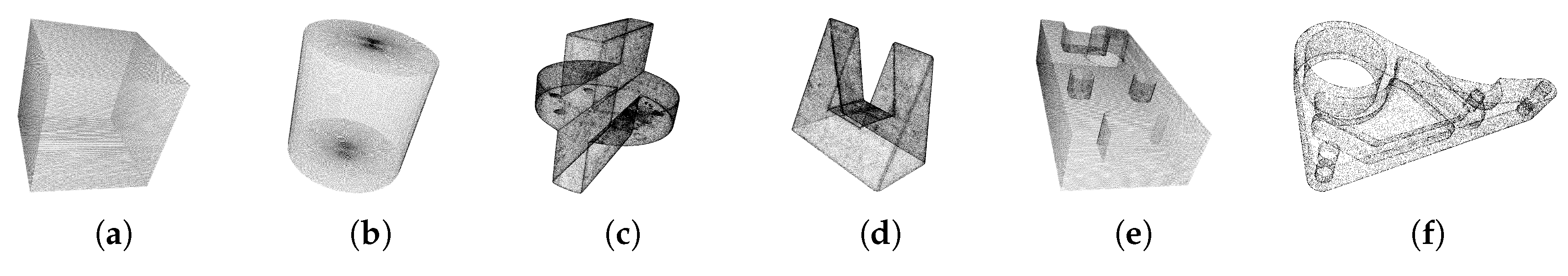
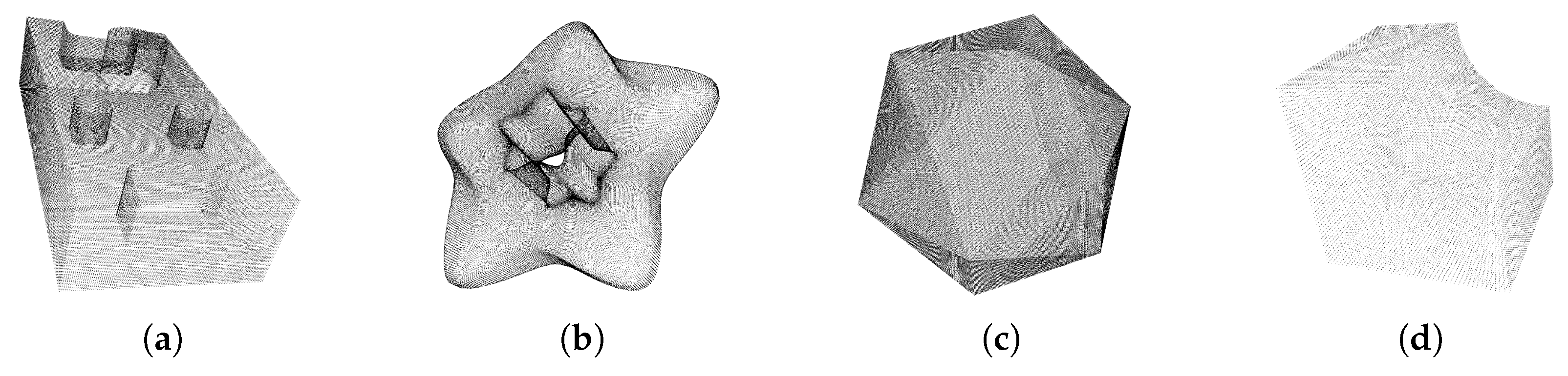
Usually, 3D scanners are provided with software that creates a physical object in the two-phase setup: reconstructing CAD model from the scanned point data, and subsequent STL model output. However, the implemented methods are usually sufficient only for simple and smooth objects. More complex objects with holes, sharp edges or corners often require prior knowledge of how to edit the scanned data. The data post-processing is time-consuming and can potentially lead to errors. We present an algorithm that automatically detects sharp features in arbitrary point cloud data. Our algorithm is based on a modified region-growing method. The input value to the algorithm is only one parameter—the normal vector threshold ${\theta }_N$ (optimal start value and the description is presented in Section 2.1). Region-growing algorithm eliminates the planar points and the remaining points are probably edge points.

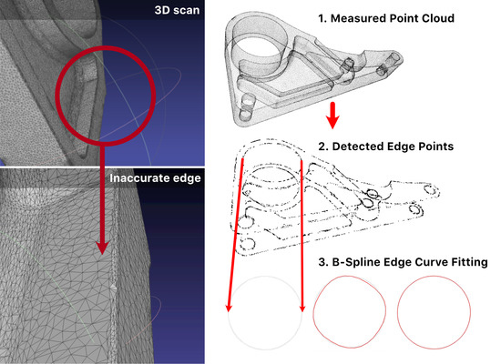
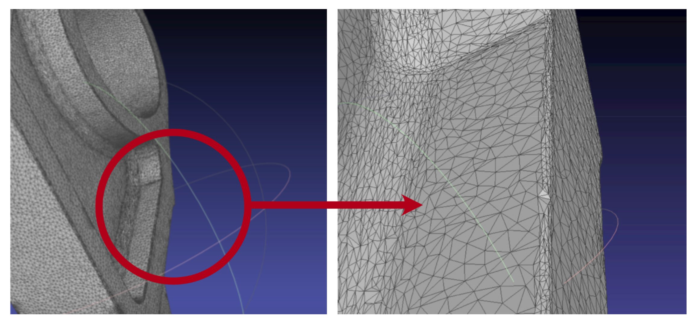
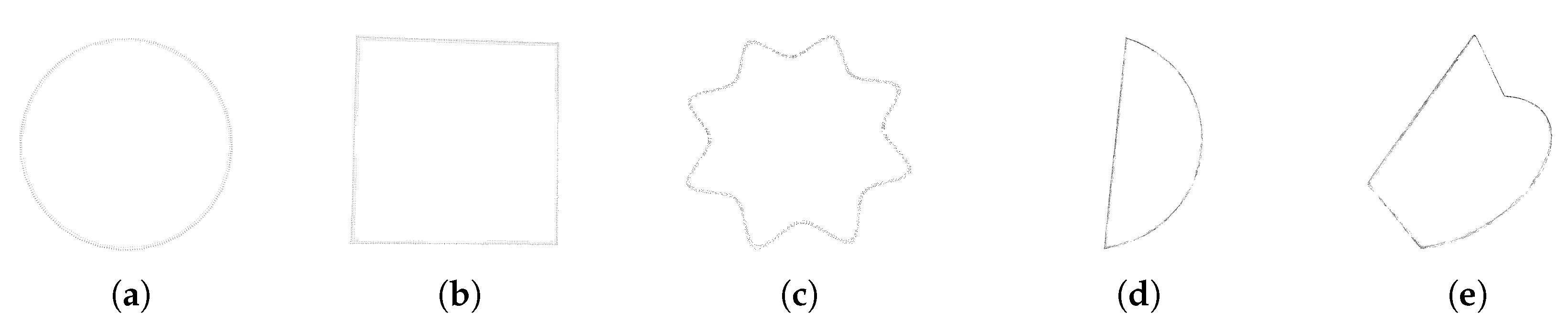
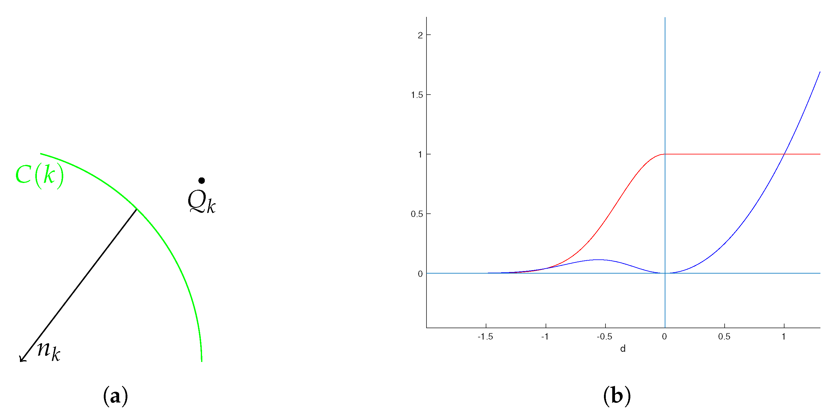
Before the final manufacturing process or 3D printing, a correct model is essential for STL generation [5] and subsequent slicing [4,6]. Figure 2 shows the common problematic part (jagged and inaccurate borders) that occurs frequently. To solve this problem, in Section 3.2 we propose the novel edge representation based on B-spline approximation. The asymmetric error evaluation is based on bell function with weighting using golden ratio [7] to improve the edge representation of the models.

Moreover, our B-spline approximation is also sufficient for direct STL slicing from point clouds that extracts the sectional contours (curves) directly without model reconstruction. The overview of these methods is e.g., in [8]. The presented B-spline approximation can be used without limitations in this slicing procedure because it obviously iteratively minimizes the shape-error of the layer curves.

Prior Work

Point cloud segmentation and classification plays a key role in point cloud processing in RE/RP usage. Segmentation is the process of grouping point clouds into multiple homogeneous regions with similar properties whereas classification is the step that labels these regions. Segmentation methods are divided into many categories and the choice of the methods depends on the area of interest, sampling density, data quality and explicit structure of point cloud. We can use the categorization described in [9,10]: region-growing, edge-based methods, model fitting, and hybrid methods.

Most of the methods start with region growing that was purposed by Besl [11] for segmentation of images. The region-growing algorithm was later expanded into 3D in two different versions: unseeded [12] and seeded [13]. Region growing is applied in plenty of different applications, e.g., extracting features and planar surfaces from 3D outcrop point clouds [14], surface segmentation, and edge feature lines extraction from fractured fragments of relics [15] or urban environment modelling [16] and also 3D city modelling (literature survey e.g., in [17]).

Region growing is frequently improved. For example, Demaris et al. [18] detect the closed sharp edges using the region growing with normals given by building a local mesh and least-squares planes through the nearest neighborhood points. The correct edge detection in provided by graph theory (minimum spanning tree). In [16], region-growing step is performed on an octree-based voxelized input point cloud representation to extract major segments.

The edge-based methods are usually used with point clouds transformed into the range images [19]. Using the high-level features (scan line grouping technique) as segmentation primitives instead of individual pixels ensure the high computational speed. However, this edge detection is not applicable for noisy data.

Model fitting methods assume that a surface can be described as a composition of simple, canonical geometric shapes (watertight reconstruction). Elementary methods use RANSAC to robustly find planes, spheres, cylinders, cones, and torii [20]. However, there occurs a problem with noise, any fine-grained details are likely to be treated as noise with the primitive prior, if they are unable to be represented as a union of smaller primitives (a survey is described in [21]). The partial solution is hybrid methods that employ primitives with other prior [22].

Region-growing, edge-based methods and model fitting do not need pre-processing, but there exist other segmentation methods based on pre-processing. These algorithms are capable of reconstructing data incompleteness [23,24] or construct a triangular mesh of given point cloud [25,26,27]. Afterwards, the formed mesh can be processed using e.g., the discrete differential geometry where local extreme of the surface detect the edge lines [25] or algebraic methods based on bivariate polynomials [27]. We must note that some of these methods work with the machine learning methods [28].

After the point cloud segmentation and classification, we need a correct model representation and tessellation (usually STL) with subsequent slicing to extract layer-based additive manufacturing [29]. There exist various approaches that combine different technologies. Traditional STL approach is described e.g., in [30]. B-spline or NURBS surfaces are used frequently, e.g., authors in [31,32] presents direct slicing from NURBS without STL. Also, B-Rep model composed of planes, spheres, cylinders and cones from a 3D mesh is fitting for slicing [33,34]. Some of the authors omit the model reconstruction and make the direct generation of sectional contour. For example, authors in [35] employ the curve skeleton of the model to slice through the surface mesh edges. B-spline curve fitting of the layers where the curve curvature is determined by a circle fitting procedure is presented in [8].

The development of neural networks and deep learning also touches the research in point cloud analysis. Some methods are promising but there is still no one-size-fits-all approach. Reviews of the methods are covered e.g., in [36,37,38].

Present literature contains most of the recently known principles. Main scientific contribution is in their improvements and applications. For example, work [39] (published 2020) uses B-spline representation and normal computation using normal curvature directly computed by partial derivatives of the surface. The omitting of the pre-defined threshold value is the main idea in [40] (published 2019). The authors suggest the composition of spatial FFT-based filtering and boundary detection, which together allow for direct generation of low noise tessellated surfaces from point cloud data. Ref [41] presents the feature sensitive point cloud simplification that is based on insensitive support vector regression.

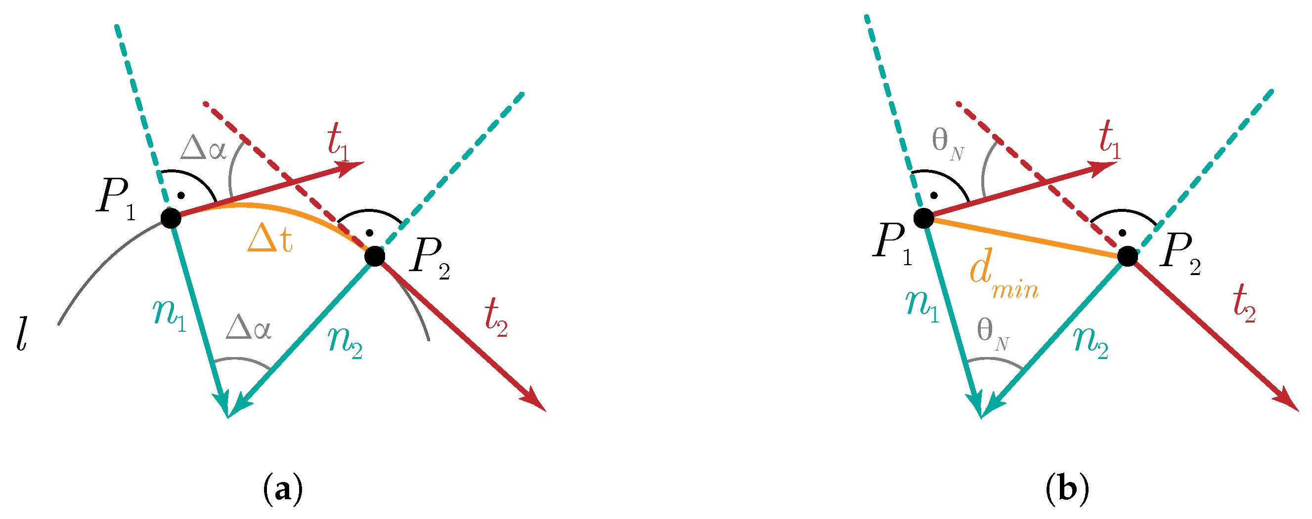
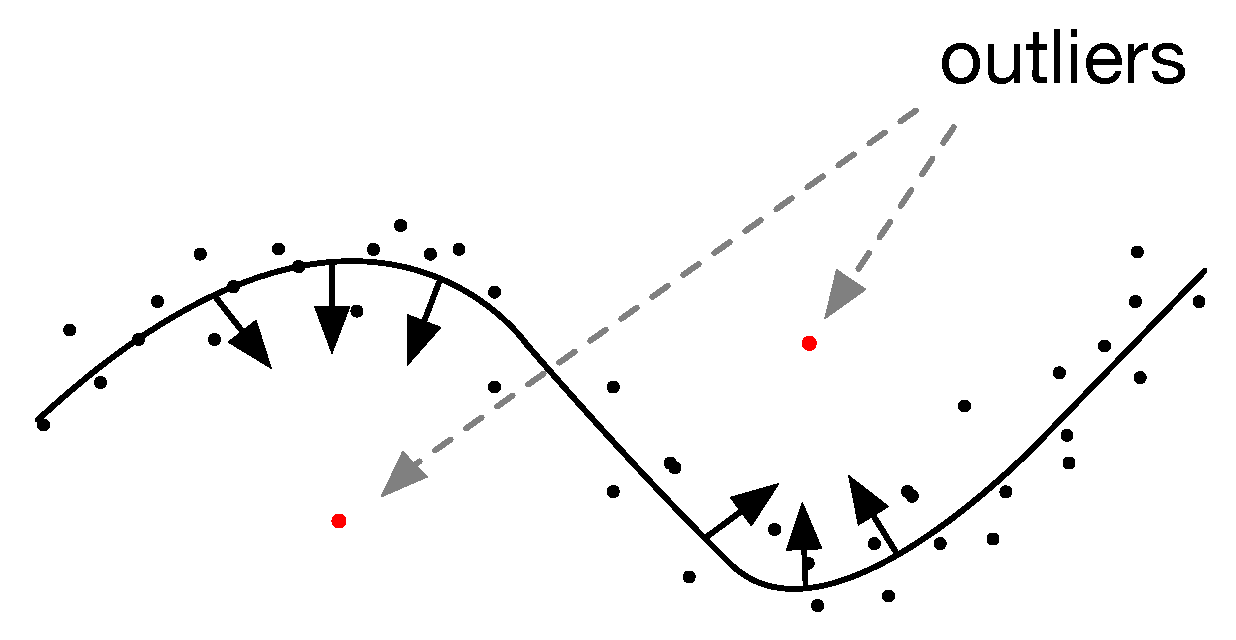
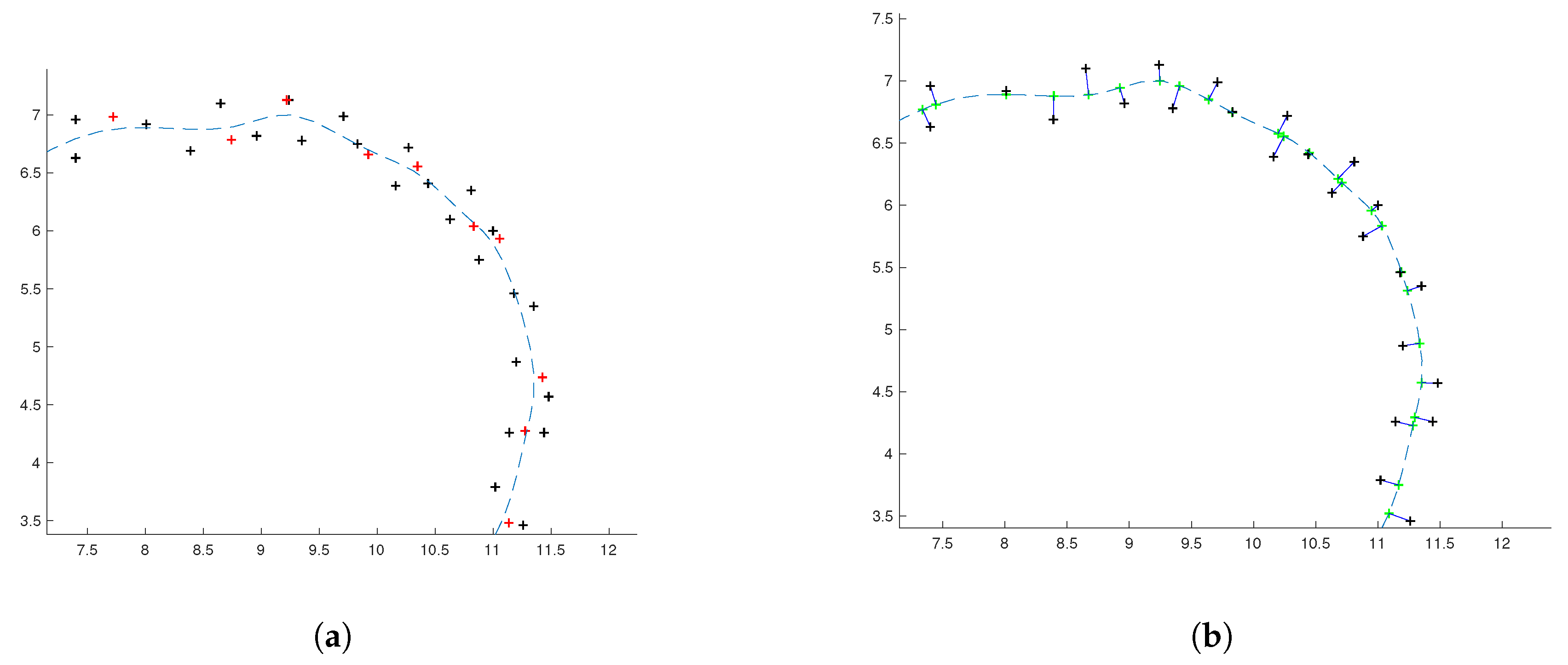
The advantages of the well-known methods (region-growing or PCA) are obvious—robustness, computed easiness, stable algorithms. Because of that, we chose these classical methods and our main idea was (1) the simplification and automatic setting of input values (described in Section 2.1) (2) find optimal error evaluation in B-spline representation that is suitable for engineering objects. The problem of error computation is described in Section 2.2 and we proposed asymmetric weighting based on golden ration.

2. Methods and Materials

The common industrial engineering components consist of flat, smooth or curved surfaces. A measurable difference in surface normals or curvature is relatively small on most of the model surfaces. Contrary to that, in the neighborhood of a sharp feature, such as a sharp edge or corner, there is a significant change in the surface normal and curvature. Thus, if we remove all points of the flat, smooth or curved surfaces, the remaining ones are the points on the sharp features. With this idea in mind, we build our method, similarly to [42], on the analysis of the eigenvalues of the covariance matrix for every point’s k-nearest neighbor. We use region growing not to find planar surfaces or regular models [43] but to remove the points with low curvature (Section 2.1).

The important input values of region growing are normal and curvature thresholds. Their setting substantially changes the segmentation results, but their choice is unintuitive and difficult especially for beginners. We find the geometric correlation between these two values and we compute the optimal initial value that is applicable in the case of regular engineering objects. This is described in the following subsections. This approach is robust to the noise and is suitable for subsequent B-spline approximation.

The B-spline approximation was chosen due to its good properties and well-known computation. The iterative process ensures sufficient quality. The error computation is based on the asymmetrically weighted distance (asymmetric distance is presented in [44]) but in our case, the weight is described with the golden ratio. The asymmetric measurement replaces the outliers and protects the curve from the zig-zag effect. This approach is described in Section 2.2. Computed B-spline curve can represent edges in point clouds. Moreover, described B-spline approximation is also possible to use in the methods for direct slicing.

2.1. Edge Points Detection

The processing of a given point cloud starts with the region-growing segmentation. Surface normal computation is based on Principal Component Analysis (PCA) [45] that uses an orthogonal transformation to convert a set of observations of possibly correlated variables into a set of values of linearly uncorrelated variables. The description is in Section 2.1.1.

Edges can be also classified by Gauss mapping [42,46,47]. The point normal vectors are projected on the Gauss sphere and subsequent clustering distinguish the point type (corner, edge, planar). This method is time-consuming so that we use the region growing.

2.1.1. PCA—Normal Estimation

The first step in the PCA algorithm is the computation of the covariance matrix C for each point P in the point cloud.

$$C=\frac{1}{k}\sum _{i=1}^k(P_i-\overline{P})·{(P_i-\overline{P})}^T,$$

(1)

where $\overline{P}$ is the centroid of k-nearest neighborhood points $P_i,i=1,2,\cdots k$ of a point P. Eigenvalues (${\lambda }_0,{\lambda }_1,{\lambda }_2$) and eigenvectors ($\overrightarrow{v_1},{\overrightarrow{v}}_2,{\overrightarrow{v}}_3$) of this matrix defines the covariance ellipsoid. We distinguish between these three cases:

• $({\lambda }_0\le {\lambda }_1\le {\lambda }_2)\wedge ({\lambda }_1\approx {\lambda }_2)$
• $({\lambda }_0\le {\lambda }_1\le {\lambda }_2)\wedge ({\lambda }_0\approx {\lambda }_1)$
• $({\lambda }_0\le {\lambda }_1\le {\lambda }_2)\wedge ({\lambda }_0\approx {\lambda }_1\approx {\lambda }_2)$.

These types of covariance ellipsoids define the neighborhood of the given point (Figure 3a–c). In the case of an oblate ellipsoid ($({\lambda }_0\le {\lambda }_1\le {\lambda }_2)\wedge ({\lambda }_1\approx {\lambda }_2)$), the point is obviously on an almost planar area and the eigenvector corresponding with the smallest eigenvalue is point normal.

2.1.2. Region Growing—Initial Normal Threshold Value $th{r}_{{\theta }_N}$

Region-growing segmentation algorithm usually requires input parameters: minimal and maximal cluster size, k-nearest neighbor points, normal threshold $th{r}_{{\theta }_N}$ and curvature threshold $th{r}_{{\theta }_C}$. Value ${\theta }_N$ is the angle between two-point normals and ${\theta }_C$ is curvature. They strongly affect the segmentation results and geometrically, they are tightly connected. The setting of the initial values is unintuitive and not user-friendly so that we focus on the optimal automatic estimation of ${\theta }_N$.

Figure 4a shows the definition of the curvature $\theta$ of the curve l at the point $P_1$. In the limit as $\Delta t\to 0$, we obtain:

$$\theta =\underset{\Delta t\to 0}{lim}\frac{\Delta \alpha }{\Delta t}$$

(2)

In the case of a point cloud, we consider the parameter $\Delta t$ as the minimal distance $d_{min}$ of the line between two adjacent points (Figure 4b). The curvature ${\theta }_C$ is computed by

$${\theta }_C=\frac{{\theta }_N}{d_{min}}.$$

(3)

Therefore, the region-growing segmentation can be controlled only by one parameter—the normal vector threshold $th{r}_{{\theta }_N}$. The following part describes the process of the ideal initial value of $th{r}_{{\theta }_N}$.

We prepared a set of testing point clouds $M_i,i=1,2,\dots ,6$ to cover the spectrum of different shapes from simple one to the complex ones (Figure 5). These point cloud data were acquired by ATOS Compact Scan 2M.We set a testing range of maximal values of normal vector threshold $th{r}_{{\theta }_N}=1,\dots ,15$. It means that the segmentation removes all points in clusters where the normal vector threshold is lower than $th{r}_{{\theta }_N}$. Let $n_{out}$ be a number of the removed points and $n_{in}$ be several points in a point cloud.

We applied the region-growing algorithm on our data-sets with parameters $th{r}_{{\theta }_N}$ and we computed the number of removed points $n_{out}$. The percentage of remaining points is defined as:

$$per{c}_N=\frac{n_{out}}{n_{in}}·100.$$

(4)

We notice that the dependence between $th{r}_{{\theta }_N}$ and $per{c}_N$ has logarithmic progress, the logarithmic regression is the best choice to compute the dependence:

$$th{r}_{{\theta }_N}=b_{1}ln\left(per{c}_N\right)+b_0,b_0,b_1\in \mathbb{R}.$$

(5)

The graphs and final results are in Section 3.1.

2.2. B-Spline Edge Representation

B-spline fitting belongs to the favorite tools for processing of a set of unorganized, possibly noisy data points in computer graphics, computer vision and CAD/CAM. The main advantage of B-spline approximation is based on the well-known formulation of B-spline [48]:

$$C\left(u\right)=\sum _{i=0}^n{B}_{i,p}\left(u\right)P_i,$$

(6)

where $B_{i,p}\left(u\right)$ is the B-spline basis function of degree p with control points $P_i$. The parameter u is from the nonperiodic and nonuniform knot interval $\mathbf{u}=<u_0,u_1,\dots ,u_{n+p+1}>$. We set $u_0=0$ and $u_{n+p+1}=1.$

Let ${\left\{Q_k\right\}}_{k=0}^m$ be the set of input points. The fitting algorithm search for control points $P_i$, knot vector $\mathbf{u}$ of the spline curve defined in Equation (6) and also the parameters $\widehat{\mathbf{u}}={\left\{{\widehat{u}}_k\right\}}_{k=0}^m$ that satisfied the equation:

$$Q_k=\sum _{i=0}^n{B}_{i,p}\left({\widehat{u}}_k\right)P_i$$

(7)

and $C\left(u_0\right)=C\left(0\right)=Q_0$, $C\left(u_{n+p+1}\right)=C\left(1\right)=Q_m$.

First, we compute the initial curve shape. The authors in [44] work with the initial circle (center of the circle is at the mean of the point cloud, the radius of the maximal distance of a point to center) or an ellipse which the main axes are computed by PCA. We start with frequently used chordal and centripetal method. The chordal method computes the parameters as:

$${\widehat{u}}_0=0;{\widehat{u}}_m=1;{\widehat{u}}_k={\widehat{u}}_{k-1}+\frac{|Q_k-Q_{k-1}|}{d}$$

(8)

where $d={\sum }_{k=1}^m|Q_k-Q_{k-1}|$. Centripetal method is similar, we only add square root of the line length. Centripetal method is more relevant in case that the data takes sharp turns.

Secondly, we set the knot vector $\mathbf{u}$ with condition that every knot span contains at least one ${\widehat{u}}_k.$ The internal knot spans are defined by [49]:

$$\begin{array}{ccc}\hfill i& =& floor\left(jd\right),\alpha =jd-i,\hfill \\ \hfill u_{p+j}& =& (1-\alpha ){\widehat{u}}_{i-1}+\alpha {\widehat{u}}_i,j=1,\dots ,n-p\hfill \end{array}$$

(9)

and function $floor$ is the largest integer such $i\le jd.$

Subsequently, coordinates of the control points $P_i$ are approximated by the standard technique of linear least-squares fitting [48]. We minimize the function:

$$f=|\sum _{k=1}^{m-1}{Q}_k-C\left({\widehat{u}}_k\right){|}^2$$

(10)

We can describe the solution in matrix form (the system of $n-1\times n-1$ equations) as:

$$\left(B^{T}B\right)\mathbf{P}=\mathbf{R}$$

(11)

where matrix BB represents the B-spline function of degree p evaluated for all ${\widehat{u}}_k$, $k=1,\dots ,n-1$. Matrix $\mathbf{P}$ are wanted control points and vector $\mathbf{R}$ is the vector of $n-1$ points:

$$\mathbf{R}=\left[\begin{array}{c}{\sum }_{k=1}^{m-1}{B}_{1,p}\left({\widehat{u}}_k\right)R_k\\ ⋮\\ {\sum }_{k=1}^{m-1}{B}_{n-1,p}\left({\widehat{u}}_k\right)R_k\end{array}\right]$$

(12)

and

$$R_k=Q_k-B_{0,p}\left({\widehat{u}}_k\right)Q_0-B_{n,p}\left({\widehat{u}}_k\right)Q_m,k=1,\dots ,m-1.$$

(13)

The Equation (11) can be solved by Gaussian elimination because the matrix $B^{T}B$ is positive definite and well-conditioned.

We must deal with the main problem throughout the iteration process: a choice of the distance measure to error determination. The formulation of the problem is simple, we have unorganized data points (in our case possible edge points) with non-uniform distribution with considerable noise. This problem can be formulated as a nonlinear optimization problem. Given input points ${\left\{Q_k\right\}}_{k=0}^m$, we want to compute control points $P_i$ that minimize a general objective function [44]:

$$f=\frac{1}{2}\sum _{k=1}^n{d}^2(P\left(u\right),Q_k)+\lambda f_s$$

(14)

$d^2(P\left(u\right),Q_k)$ is the distance of point $Q_k$ to the curve $P\left(t\right)$, $f_s$ is regularization term to ensure a smooth curve, $\lambda$ is weight of $f_s.$ In our algorithm, we work with the asymmetric weighted point distance measure. We introduce a novel error term in Equation (15) that is based on golden ration. It ensures that the inner points (on the same side as a normal vector) have lesser influence than the outer. This advantage eliminates the problematic outliers and improves the shape of the curve (Figure 6).

The distance $d_k$ is the signed distance of the point $Q_k$ and the closest point on the computed B-spline curve. $d_k$ is positive if the point $Q_k$ is on the same side as normal $n_k$—see Figure 7a. This error term is:

$$w_{\phi }\left(d_k\right)=\left\{\begin{array}{cc}{\left(\frac{1}{\phi }+\phi \right)}^{-\frac{d_k^2}{{\sigma }^2}}\hfill & \mathrm{for}{d}_k<0\hfill \\ 1\hfill & \mathrm{for}{d}_k\ge 0\hfill \end{array}\right.$$

(15)

$k=0,1,2\cdots ,m$, where $\sigma$ defines the width of the transition of the weighting function with respect to the signed distance. The value $\phi$ is the golden ratio $1.61803398875.$ The objective function has a form:

$$f_{\phi }=\sum _{k=0}^m{w}_{\phi }\left(d_k\right)d_k^2,$$

(16)

The weighting function $w_{\phi }\left(d_k\right)$ and objective function $f_{\phi }$ are modelled in Figure 7b.

The asymmetric error detects the parts where the curve accuracy is insufficient. The improvement is done by local knot insertion. We know the parameter ${\overline{u}}_k$ of the nearest curve point $C\left(\overline{u_k}\right)$ for every $Q_k.$ Therefore, we insert all knots $\overline{u_k}$ in the insufficient parts and recompute the curve using knot insertion scheme. If $\overline{u_k}\in <u_k,u_{k+1})$, then the new control points ${\overline{P}}_i$ are:

$${\overline{P}}_i={\beta }_i{P}_i+(1-{\beta }_i)P_{i-1}$$

(17)

where

$${\beta }_i=\left\{\begin{array}{cc}\frac{{\overline{u}}_k-u_i}{u_{i+p}-u_i}\hfill & \mathrm{for}k-p+1\le i\le k\hfill \\ 1\hfill & \mathrm{for}i\le k-p\hfill \\ 0\hfill & \mathrm{for}i\ge k+1\hfill \end{array}\right.$$

(18)

In the parts, where the error is high, we add the new knot in the value of the nearest curve point. We tested the proposed improvement on the set of point clouds $C_1,C_2,C_3,C_4$ and $C_5$. The test results and thorough comparison are in Section 3.

3. Results and Discussion

This section contains two main parts: Estimation of normal threshold parameter and B-spline fitting with a novel asymmetric error. In the first part, we made a series of testing objects—from almost planar ones to the complex ones with holes. We proceeded these models with region-growing algorithm and using our proposed method (Section 2.1.2) we estimate the optimal value of the normal threshold. This value can be set as a universal input threshold value. The inexperienced end-users of the edge detection algorithm do not need any complex manual on how to control the results.

The second step contains a B-spline fitting algorithm for the edge representation. The input of this part are points detected in the first step. The asymmetric error with the golden ratio (Equation (15)) is used in the iteration process as described in the previous section. On the set of different curves (smooth, complex) we show the results and we make a comparison with method [44].

Feature detection algorithm was implemented in Microsoft Visual Studio C++ with Point Cloud Library 1.8.0. The B-spline approximation was programmed in MATLAB R2018a. The point cloud data-sets were obtained by ATOS Compact Scan 2M. Testing was provided on the MacBook Pro, 2.6 GHz Intel Core i7, 16 GB 1600 MHz DDR3, NVIDIA GeForce GT 750M 2048 MB, SSD.

3.1. Estimation of Normal Threshold $th{r}_{{\theta }_N}$

The first analyses examines the impact of parameter $th{r}_{{\theta }_N}$. The set of testing point clouds $M_i,i\in \langle 1,6\rangle$ is in Figure 5. Let $s_{in}$ be several points in the given point cloud (

Table 1. The point clouds with number of points $s_{in}$.

Model	${\mathit{M}}_1$	${\mathit{M}}_2$	${\mathit{M}}_3$	${\mathit{M}}_4$	${\mathit{M}}_5$	${\mathit{M}}_6$
$s_{in}$	87,848	67,394	195,815	123,112	103,534	90,209

).

We applied the region-growing algorithm on our data-sets with the initial parameters $th{r}_{{\theta }_N}\in \mathbb{N}$, $th{r}_{{\theta }_N}=1,\dots ,15$ and we find the number of removed points $n_{out}$. The percentage of remaining points is computed by:

$$per{c}_N=\frac{n_{out}}{n_{in}}·100.$$

(19)

Table A1. Table of $th{r}_{{\theta }_N}$ and $per{c}_N$ for all testing point clouds.

${\mathit{thr}}_{{\mathit{\theta }}_{\mathit{N}}}$		0.5	2	4	6	14
$M_1$
$per{c}_N$		4.71	1.57	0.47	0.05	0.02
$M_2$
$per{c}_N$		4.34	3.36	1.71	0.85	0.85
$M_3$
$per{c}_N$		26.54	16.38	3.24	0.56	0.01
$M_4$
$per{c}_N$		29.27	18.65	2.87	0.38	≈ 0
$M_5$
$per{c}_N$		10.41	6.56	4.04	2.03	0.06
$M_6$
$per{c}_N$		67.14	37.25	14.10	5.09	0.09

provides the results obtained by the analysis of different values $th{r}_{{\theta }_N}$. We can see that the value of $per{c}_N$ is tightly related to the complexity of the model.

Table A2. Table of data and logarithmic regression for all testing point clouds.

Model	Chart	Regression
$M_1$		$-2.06·\ln \left(x\right)+4.10$
$M_2$		$-4.87·\ln \left(x\right)+8.39$
$M_3$		$-1.50·\ln \left(x\right)+5.57$
$M_4$		$-1.28·\ln \left(x\right)+5.21$
$M_5$		$-2.43·\ln \left(x\right)+7.01$
$M_6$		$-1.92·\ln \left(x\right)+9.07$

(middle column) presents point charts of the values $th{r}_{{\theta }_N}$ and $per{c}_N$. We can see that independently on the model complexity, it has the logarithmic progress. Therefore, the dependence between $th{r}_{{\theta }_N}$ and $per{c}_N$ can be generally described with logarithmic regression using Equation (5). The final equations and graphs are in Table A2 (last column).

We want to determine the best possible input value $th{r}_{{\theta }_N}$ that is applicable for common point clouds of the engineering models. We start with the average regression equation (the average of the equations in Table A2):

$${\theta }_{ST}\approx R\left(x\right)=-2.45·\ln \left(x\right)+6.06.$$

(20)

The optimal value of $perc$ is set empirically as 1–6%. Therefore, the values of $th{r}_{{\theta }_N}$ are in interval $\langle R\left(1\right),R\left(6\right)\rangle$. Obviously, we get:

$$\begin{array}{ccc}R\left(1\right)=-2.45·\ln \left(1\right)+6.06& \le {\theta }_{ST}\le & -2.45·\ln \left(6\right)+6.06=R\left(6\right)\\ 6.06& \le {\theta }_{ST}\le & 1.67.\end{array}$$

(21)

The arithmetic mean of $\mathbb{R}\left(1\right)$ and $\mathbb{R}\left(6\right)$ is ${\theta }_{opt}=3.86$ is set as a default initial value in the proposed feature detection algorithm. In the case of insufficient results, this value can be changed incrementally.

Table 2. The final segmentation using the initial value ${\theta }_{opt}=3.86$.

	Input	Output		Input	Output
$M_1$			$M_2$
$M_3$			$M_4$
$M_5$			$M_6$

shows the segmentation results for models $M_i,i=1,2,\dots ,6$ using the default initial value ${\theta }_{opt}=3.86$. It is obvious that the results are sufficient and this value helps inexperienced users to start segmentation without any prior knowledge of curvature or normal threshold. By applying the incremental change of this value, the results are improved to obtain sufficient quality for actual use.

We made a comparison of our method with similar approaches presented in [18,47]. We built a similar set of models for the evaluation (see Figure 8). The initial value of the curvature threshold was set to the pre-defined initial value ${\theta }_N$ and this value was incrementally changed to obtain the best results.

In

Table 3. The comparison of the testing results (upper row: model from [18,47]), bottom row: edge detection with the incremental change of the threshold value).

(a)	(b)	(c)	(d)
$th{r}_{{\theta }_N}=4$	$th{r}_{{\theta }_N}=1.2$	$th{r}_{{\theta }_N}=1$	$th{r}_{{\theta }_N}=1.5$

, model in column (a), there is significant difference between the results—the incorrectly detected cylinder parts in results [18]. Our method with $th{r}_{{\theta }_N}=4$ provides visibly better results.

Models (b), (c) and (d) are similar to models in [47]. We can see that our method provides comparable results. In the case of these models, we had to decrease the value of ${\theta }_N$ because these models contain a lot of planar surfaces.

3.2. B-Spline Curve Fitting

This section presents the results of the proposed B-spline approximation described in Section 2.2. We tested the computation on the set of curves $C_i$, $i=1,\dots ,5$ (Figure 9). The curves were extracted from point clouds—square curve (200 × 200 mm) from the cubic model, circle (radius 200 mm) from the cylindrical model. Remaining models were generated in Blender studio to prove the versatility of the algorithm.

Table 4. The testing curves—number of points $s_{in}$.

Model Curve	${\mathit{C}}_1$	${\mathit{C}}_2$	${\mathit{C}}_3$	${\mathit{C}}_4$	${\mathit{C}}_5$
$s_{in}$	1632	1307	2560	2477	3130

gives the numbers of points of these curves.

The set of curve points was tested using presented B-spline curve fitting with adaptive knot insertion. The most difficult part was the optimal setting of the error computation—how to measure the quality of approximation if we do not know the correct shape. The common approach of the error computation works with point distance that offers the robustness. The tangent distance [50] provides the substantially faster convergence. The squared distance with asymmetric weighting [44,51] benefits from both and performs a stable method. We used the asymmetric weighting, but we proposed a novel evaluation of asymmetric error:

$$f_{\phi ,k}^2=w_{\phi ,k}\left(d_k\right)d_k^2,\mathrm{where}{w}_{\phi }\left(d_k\right):=\left\{\begin{array}{cc}{\left(\frac{1}{\phi }+\phi \right)}^{-\frac{d_k^2}{{\sigma }^2}}\hfill & \mathrm{for}{d}_k<0\hfill \\ \phantom{(}\hfill & \phantom{(}\hfill \\ 1\hfill & \mathrm{for}{d}_k\ge 0\hfill \end{array}\right.$$

(22)

$$k=0,1,2\cdots ,m,$$

We set the error threshold to 1 mm. In Figure 10a, we can see the initial B-spline curve (dashed blue line) that is computed by the chordal method and least square method described in Section 2.2. Red points are new B-spline control points and black crosses are the points in the point cloud. Figure 10b shows the distance of the point cloud points to the fitting curve (blue line segments).

The value of asymmetric error determines whether we proceed the knot insertion and insert new control points in the inaccurate positions. Figure 11 shows the result of second iteration of B-spline fitting. We implemented the method [44] and proposed computation given by Equation (22). We computed average error of approximation $E_m$ and $E_{gold}$ in

Table 5. Computation of approximation error $E_m$ and $E_{gold}$ using different values of $\sigma$.

$\mathit{\sigma }$	0.02	0.09	0.1
$E_m$	0.9387	0.9661	0.9702
$E_{gold}$	0.9382	0.9560	0.9604

(we set $\sigma =0.02,0.09,0.1$). We can see that in the case of $\sigma =0.09$ and $\sigma =0.1$ the error is lower and the shape of the curve is visibly better (see Figure 11).

Table A3. Comparison of B-spline curve approximation of testing clouds, CP is number of control points, $w_{\phi }$ is average weighted error.

$C_1$
CP	4	10	20
$w_{\phi }$[mm]	2.35	1.15	0.83
$C_2$
CP	4	10	20	40	80
$w_{\phi }$[mm]	14.01	5.54	2.02	1.25	0.99
$C_3$
CP	20	40	80
$w_{\phi }$[mm]	3.96	0.96	0.85
$C_4$
CP	80	100	160
$w_{\phi }$[mm]	0.41	0.37	0.27
$C_5$
CP	10	40	80
$w_{\phi }$[mm]	2.19	0.67	0.33

shows different results with the number of control points and the corresponding asymmetric error. It is obvious that the algorithm is applicable in the case of different structures and work well with corner points.

4. Conclusions

The main contribution of this article is a method that improves the detection and representation of the edges of scanned engineering parts. This area is challenging because the scanning device (usually a 3D scanner) is frequently not able to cover the sharp edges with a sufficient amount of measured points. Therefore, the used techniques have a problem with the correct representation of the object shape. A manual time-consuming work in some commercial program is needed for fine-tuning of the scanned objects. Our article describes the overall workflow of the automatic edge detection in the arbitrary point cloud and subsequent correct edge representation using splines. We provide a user-friendly solution based on a single control parameter that can work with different shapes of engineering parts as well as other 3D scans generally. This method is also suitable e.g., for the reconstruction of the sharp edges of the buildings based on airborne laser scanning. The density of the measured points is also limiting the ability of the algorithms to reconstruct the precise shape of the walls. Simple adjustment of a single control parameter for the particular type of scanned object can substantially improve the results.

As the first step of our algorithm, we used the standard region-growing segmentation. We improved the part of principal component analysis (PCA) algorithm that is necessary for normal computation. We made a series of tests with variable shapes (from almost planar to complex ones) and using geometry calculus and numerical methods we implemented new variable—normal vector threshold $th{r}_{{\theta }_N}$. Subsequently, we set this computed optimal value as the start value. Users can change incrementally this threshold in dependence on the shape of the object. Using one interconnected value to control the result is more suitable and very comfortable for end-users that are not able to understand to all algorithm parameters. Region-growing method removes the planar points and the remaining points are the possible edge points.

The next step was challenging. How to compute the error of the edge representation when the correct edge points are missing. We chose to work with iterative B-spline method using the asymmetrically weighted point distance. The reasons are discussed in Section 3. We decided to use the golden ratio as a parameter (Section 2.2). It ensures that the inner points (on the same side as a normal vector) have lesser influence than the outer and the result is optically “perfect”. This advantage eliminates the problematic outliers and improves the shape of the curve. We made the algorithm resistant to noise and prevented the zig-zag effect.

Our work has many possible extensions. Reverse engineering is tightly connected with 3D printing technology. Printed object correctness depends on the appropriate slices (G-code). The first follow-up can be an adjustment of the B-spline slicing method. Furthermore, the visualization of the scanned objects can be improved. Approximation of the curve points can be added to the triangulation net. Substantial advance can be an incorporation of the T-splines. T-spline enables irregular grid and we can represent sharp edges using different local knot vectors. Certainly, many scientific areas take advantage of huge progress in neural networks and deep learning. Point cloud analysis is not an exception. We follow the research in this area but the usage is now limited by the sensitivity of parameters and most methods work just with small point clouds [38].

References

1. Davis, J.; Edgar, T.; Porter, J.; Bernaden, J.; Sarli, M. Smart manufacturing, manufacturing intelligence and demand-dynamic performance. Comput. Chem. Eng. 2012, 47, 145–156. [Google Scholar] [CrossRef]
2. Vaidya, S.; Ambad, P.; Bhosle, S. Industry 4.0—A Glimpse. Procedia Manuf. 2018, 20, 233–238. [Google Scholar] [CrossRef]
3. Chua, C.K.; Leong, K.F.; Lim, C.S. Rapid Prototyping: Principles and Applications. In Rapid Prototyping: Principles and Applicationse; World Scientific Publishing: Singapore, 2010. [Google Scholar]
4. Qiu, Y.; Zhou, X.; Qian, X. Direct slicing of cloud data with guaranteed topology for rapid prototyping. Int. J. Adv. Manuf. Technol. 2011, 53, 255–265. [Google Scholar] [CrossRef]
5. Livesu, M.; Ellero, S.; Martinez, J.; Lefebvre, S.; Attene, M. From 3D models to 3D prints: An overview of the processing pipeline. Comput. Graph. Forum 2017, 36, 1–24. [Google Scholar] [CrossRef] [Green Version]
6. Choi, S.-H.; Samavedam, S. Modelling and optimisation of rapid prototyping. Comput. Ind. 2002, 47, 39–53. [Google Scholar] [CrossRef]
7. Sen, S.K.; Agarwal, R.P. Golden ratio in science, as random sequence source, its computation and beyond. J. Comput. Math. Appl. 2008, 56, 469–498. [Google Scholar] [CrossRef] [Green Version]
8. Javidrad, R.; Pourmoayed, A.R. Contour curve reconstruction from cloud data for rapid prototyping. Robot. Comput. Integr. Manuf. 2011, 27, 397–404. [Google Scholar] [CrossRef]
9. Grilli, E.; Menna, F.; Remondino, F. A review of point clouds segmentation and classification algorithms. Int. Arch. Photogramm. Remote Sens. Spat. Inf. Sci. 2017, XLII-2/W3, 339–344. [Google Scholar] [CrossRef] [Green Version]
10. Nguyen, A.; Le, B. 3D point cloud segmentation: A survey. In Proceedings of the 6th IEEE Conference on Robotics, Automation and Mechatronics (RAM), Manila, Philippine, 12–15 November 2013; pp. 225–230. [Google Scholar]
11. Besl, P.J.; Jain, R.C. Segmentation through Variable-Order Surface Fitting. IEEE Trans. Pattern Anal. Mach. Intell. Arch. 1988, 10, 167–192. [Google Scholar] [CrossRef] [Green Version]
12. Nahar, M.; Ali Sujan Rahman, M. Improvement of Single Seeded Region Growing Algorithm on Image Segmentation. Glob. J. Comput. Sci. Technol. 2018, 18, 15–22. [Google Scholar]
13. Adams, R.; Bischof, L. Seeded Region Growing. IEEE Trans. Pattern Anal. Mach. Intell. Arch. 1994, 6, 641–647. [Google Scholar] [CrossRef] [Green Version]
14. Wang, X.; Zoua, L.; Shena, X.; Rena, Y.; Qina, Y. A region-growing approach for automatic outcrop fracture extraction from a three-dimensional point cloud. Comput. Geosci. 2017, 99, 100–106. [Google Scholar] [CrossRef] [Green Version]
15. Xu, J.; Zhou, M.; Wu, Z.; Shui, W.; Ali, S. Robust surface segmentation and edge feature lines extraction from fractured fragments of relics. J. Comput. Des. Eng. 2015, 2, 79–87. [Google Scholar] [CrossRef] [Green Version]
16. Vo, A.V.; Truong-Hong, L.; Laefer, D.F.; Bertolotto, M. Octree-based region growing for point cloud segmentation. ISPRS J. Photogramm. Remote Sens. 2015, 104, 88–100. [Google Scholar] [CrossRef]
17. Ni, H.; Lin, X.; Ning, X.; Zhang, J. Edge Detection and Feature Line Tracing in 3D-Point Clouds by Analyzing Geometric Properties. Remote Sens. 2016, 8, 710. [Google Scholar] [CrossRef] [Green Version]
18. Demaris, K.; Vanderstraeten, D.; Volodine, T.; Roose, D. Detection of closed sharp edges in point clouds using normal estimation and graph theory. Comput. Aided Des. 2007, 39, 267–283. [Google Scholar]
19. Jiang, X.Y.; Bunke, H.; Meier, U. Fast range image segmentation using high-level segmentation primitives. In Proceedings of the Third IEEE Workshop on Applications of Computer Vision, Sarasota, FL, USA, 2–4 December 1996; pp. 83–88. [Google Scholar]
20. Schnabel, R.; Wahl, R.; Klein, R. Efficent Ransac for point cloud shape detection. Comput. Graph. Forum 2007, 26, 214–226. [Google Scholar] [CrossRef]
21. Berger, M.; Tagliasacchi, A.; Seversky, L.M.; Alliez, P.; Guennebaud, G.; Levine, J.A.; Silva, C.T. A Survey of Surface Reconstruction from Point Clouds. Comput. Graph Forum 2016, 36, 301–329. [Google Scholar] [CrossRef] [Green Version]
22. Lafarge, F.; Alliez, P. Surface reconstruction through point set structuring. In Computer Graphics Forum; Benes, B., Chen, M., Eds.; Wiley: New York, NY, USA, 2013; pp. 225–234. [Google Scholar]
23. Wang, M.; Ju, M.; Fan, Y.; Guo, S.; Liao, M.; Yang, H.; Komura, T. 3D Incomplete Point Cloud Surfaces Reconstruction With Segmentation and Feature-Enhancement. IEEE Access 2019, 7, 15272–15281. [Google Scholar] [CrossRef]
24. Yin, K.; Huang, H.; Zhang, H.; Gong, M.; Cohen-Or, D.; Chen, B. Morfit: Interactive surface reconstruction from incomplete point clouds with curve-driven topology and geometry control. ACM Trans. Graph. 2014, 33, 202. [Google Scholar] [CrossRef]
25. Hildebrandt, K.; Polthier, K.; Wardetzky, M. Smooth features lines on surface meshes. In Eurographics Symposium on Geometry Processing; Desbrun, M., Pottmann, H., Eds.; Eurographics Association: Aire-la-Ville, Switzerland, 2005; pp. 85–90. [Google Scholar]
26. Ohtake, Y.; Belyaev, A. Automatic detection of geodesic ridges and ravines on polygonal surface. J. Three Dimens. Images 2001, 15, 127–132. [Google Scholar]
27. Stylianou, G.; Farin, G. Crest lines extraction from 3D triangulated meshes. In Hierarchical and Geometrical Methods in Scientific Visualization; Farin, G., Hamann, B., Hagen, H., Eds.; Springer: Berlin, Germany, 2003; pp. 69–81. [Google Scholar]
28. Tootooni, S.; Dsouza, A.; Donovan, R.; Rao, P.K.; Kong, Z.; Borgesen, P. Classifying the Dimensional Variation in Additive Manufactured Parts From Laser-Scanned Three-Dimensional Point Cloud Data Using Machine Learning Approaches. J. Manuf. Sci. Eng. 2017, 139, 142–149. [Google Scholar]
29. Beniere, R.; Subsol, G.; Gesquire, G.; Le Breton, F.; Puech, W. A comprehensive process of reverse engineering from 3D meshes to CAD models. Comput. Aided Des. 2013, 45, 1382–1393. [Google Scholar] [CrossRef] [Green Version]
30. Zhang, Z.; Sanjay, J. An improved slicing algorithm with efficient contour construction using STL files. Int. J. Adv. Manuf. Technol. 2015, 80, 1347–1362. [Google Scholar] [CrossRef]
31. Ma, W.; But, W.C.; He, P. NURBS-based adaptive slicing for efficient rapid prototyping. Comput. Aided Des. 2004, 36, 1309–1325. [Google Scholar] [CrossRef]
32. Oropallo, W.; Piegl Les, A.; Rosen, P.; Rajab, K. Generating point clouds for slicing free-form objects for 3-D printing. Comput. Aided Des. Appl. 2017, 14, 242–249. [Google Scholar] [CrossRef]
33. Shi, K.; Cai, C.; Wu, Z.; Yong, J. Slicing and support structure generation for 3D printing directly on B-rep models. Vis. Comput. Ind. Biomed. Art 2019, 2, 3. [Google Scholar] [CrossRef]
34. Zhao, G.; Ma, G.; Feng, J.; Xiao, W. Nonplanar slicing and path generation methods for robotic additive manufacturing. Int. J. Adv. Manuf. Technol. 2018, 96, 3149. [Google Scholar] [CrossRef]
35. Kresslein, J.; Haghighi, P.; Jaejong, P.; Ramnath, S.; Sutradhar, A.; Shah, J.J. Automated cross-sectional shape recovery of 3D branching structures from point cloud. J. Comput. Des. Eng. 2018, 5, 368–378. [Google Scholar] [CrossRef]
36. Liu, W.; Sun, J.; Li, W.; Hu, T.; Wang, P. Deep Learning on Point Clouds and Its Application: A Survey. Sensors 2019, 19, 4188. [Google Scholar] [CrossRef] [PubMed] [Green Version]
37. Griffiths, D.; Boehm, J. A Review on Deep Learning Techniques for 3D Sensed Data Classification. Remote Sens. 2019, 11, 1499. [Google Scholar] [CrossRef] [Green Version]
38. Guo, Y.; Wang, H.; Hu, Q.; Liu, H.; Liu, L.; Bennamoun, M. Deep Learning for 3D Point Clouds: A Survey. arXiv 2019, arXiv:abs/1912.12033. [Google Scholar] [CrossRef]
39. Lee, D.; Quan, I.; Wu, C.; Wu, J.; Tamir, D.; Rishe, N. Optimizing B-Spline Surface Reconstruction for Sharp Feature Preservation. In Proceedings of the 10th Annual Computing and Communication Workshop and Conference (CCWC), Las Vegas, NV, USA, 6–8 January 2020; pp. 359–364. [Google Scholar]
40. Mineo, C.; Pierce, S.G.; Summan, R. Novel algorithms for 3D surface point cloud boundary detection and edge reconstruction. J. Comput. Des. Eng. 2019, 6, 81–91. [Google Scholar] [CrossRef]
41. Markovic, V.; Jakovijevic, Z.; Miljkovic, Z. Feature sensitive three-dimensional point cloud simplification using support vector regression. Tech. Gaz. 2019, 27, 985–994. [Google Scholar]
42. Bazazian, D.; Casas, J.R.; Ruiz-Hidalgo, J. Fast and Robust Edge Extraction in Unorganized Point Clouds. In Proceedings of the International Conference on Digital Image Computing: Techniques and Applications (DICTA), Adelaide, Australia, 23–25 November 2015; pp. 1–8. [Google Scholar]
43. Wang, Y.X.; Wang, J.; Chen, X.; Chu, T.; Liu, M.; Yang, T. Feature Surface Extraction and Reconstruction from Industrial Components Using Multistep Segmentation and Optimization. Remote Sens. 2018, 10, 1073. [Google Scholar] [CrossRef] [Green Version]
44. Mörwald, T.; Balzer, J.; Vincze, V. Modeling connected regions in arbitrary planar point clouds by robust B-spline approximation. Robot. Auton. Syst. 2008, 76, 141–151. [Google Scholar] [CrossRef]
45. Jolliffe, I.T. Principal Component Analysis; Springer: New York, NY, USA, 1986; p. 487. [Google Scholar]
46. Banchoff, T.; Gaffney, T.; McCrory, C. Cups of the Gauss Map. In Research Notes in Mathematics; Pitman: London, UK, 1982. [Google Scholar]
47. Weber, C.; Hahmann, S.; Hagen, H. Methods for feature detection in point cloud. In Visualization of Large and Unstructured Data Sets–IRTG Workshop; Middel, A., Scheler, I., Hagen, H., Eds.; Schloss Dagstuhl–Leibniz-Zentrum fuer Informatik: Bodega Bay, CA, USA, 2010; pp. 90–99. [Google Scholar]
48. Piegl, L.; Tiller, W. The NURBS Book; Springer: New York, NY, USA, 1997. [Google Scholar]
49. de Boor, C. A Practical Guide to Splines; Springer: New York, NY, USA, 2001. [Google Scholar]
50. Blake, A.; Isard, M. The Active Contours; Springer: New York, NY, USA, 1998. [Google Scholar]
51. Wang, W.; Pottmann, H.; Liu, Y. Fitting B-spline curves to point clouds by curvature-based squared distance minimization. ACM Trans. Graph. 2006, 25, 214–238. [Google Scholar] [CrossRef]
Figure 1. Reverse engineering process.
Ijgi 09 00422 g001
Figure 2. Problematic parts on the edges.
Ijgi 09 00422 g002
Figure 3. Types of the covariance ellipsoid (a) oblate (b) prolate (c) similar to a sphere.
Ijgi 09 00422 g003
Figure 4. (a) Curvature of the curve, (b) curvature estimation in a point cloud.
Ijgi 09 00422 g004
Figure 5. Testing point clouds: (a) M ffl , (b) M 2 , (c) M 3 , (d) M 4 , (e) M 5 , (f) M 6 .
Ijgi 09 00422 g005
Figure 6. The example of the outliers.
Ijgi 09 00422 g006
Figure 7. (a) Normal vector is on the opposite side of the point Q k , distance d k is negative, (b) the graphs of the functions w φ (red line) and f φ (blue line).
Ijgi 09 00422 g007
Figure 8. Set of testing models for comparison (a) similar to model in [18], (bd) similar to models in [47].
Ijgi 09 00422 g008
Figure 9. Set of testing point clouds: (a) C 1 , (b) C 2 , (c) C 3 , (d) C 4 , (e) C 5 .
Ijgi 09 00422 g009
Figure 10. (a) The initial B-spline curve of the cloud points (black crosses) and new control points (red crosses), (b) the distance of the point cloud points and the computed curve line.
Ijgi 09 00422 g010
Figure 11. The comparison of second iteration using method [44] (red line) and proposed method given by Equation (22) (blue line). Different values of σ : (a) σ = 0.02 , (b) σ = 0.09 , (c) σ = 0.1 .
Ijgi 09 00422 g011