Multifractal Characteristics of Seismogenic Systems and b Values in the Taiwan Seismic Region

Abstract
1. Introduction
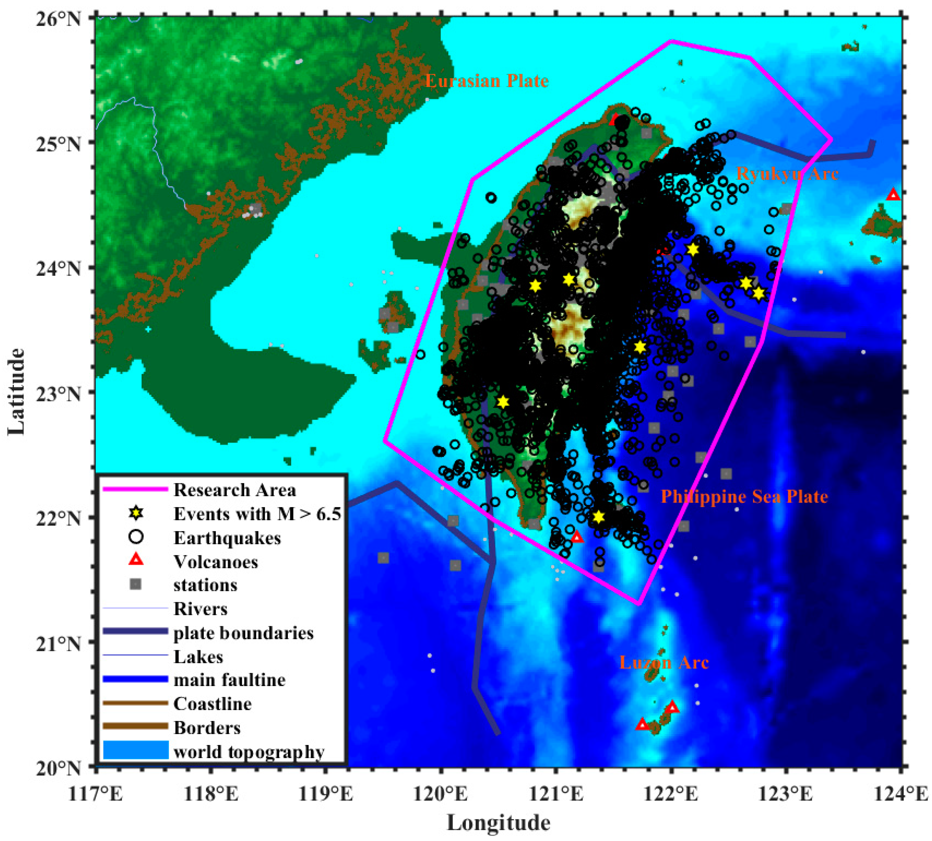
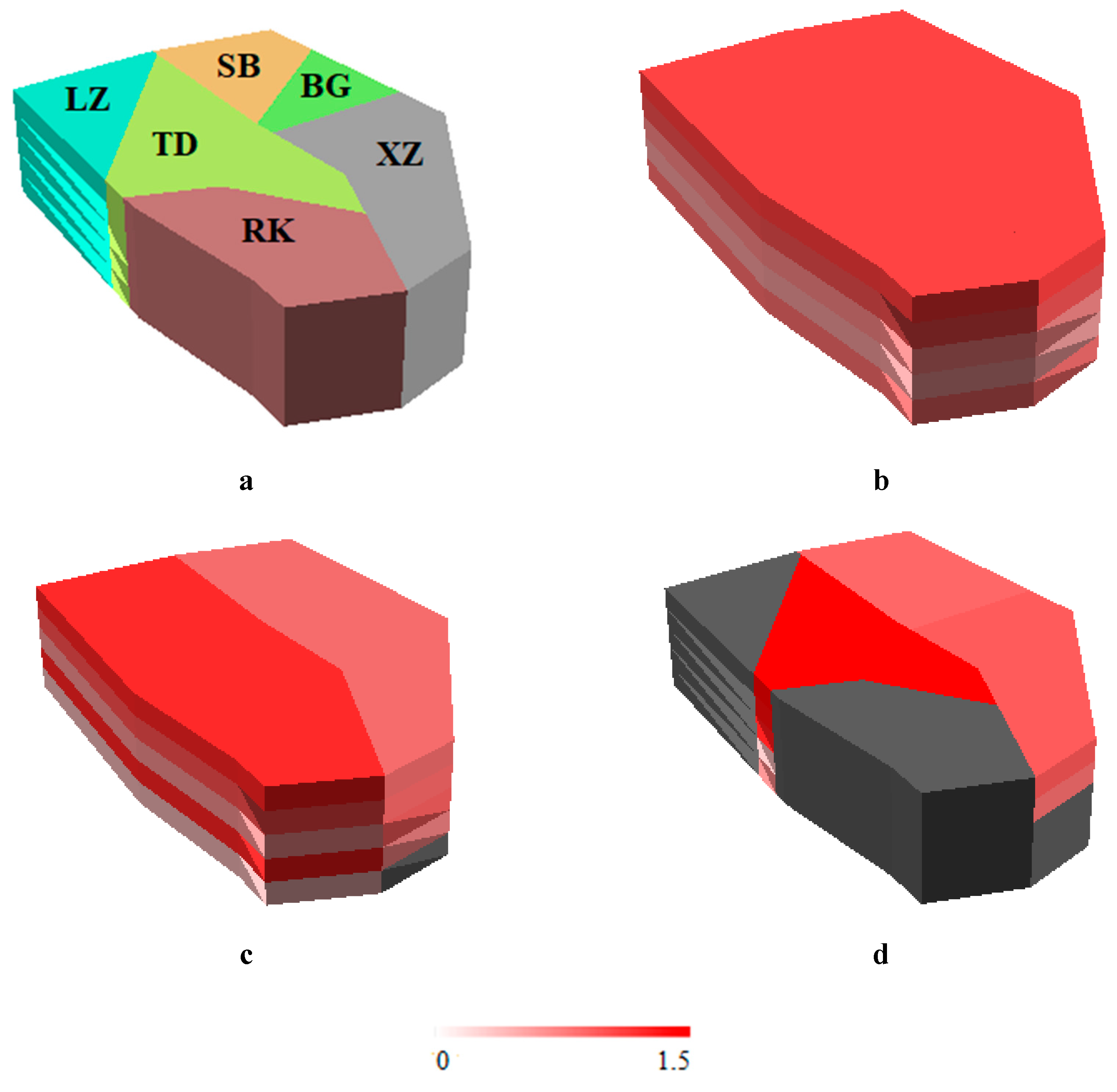
2. Study Area
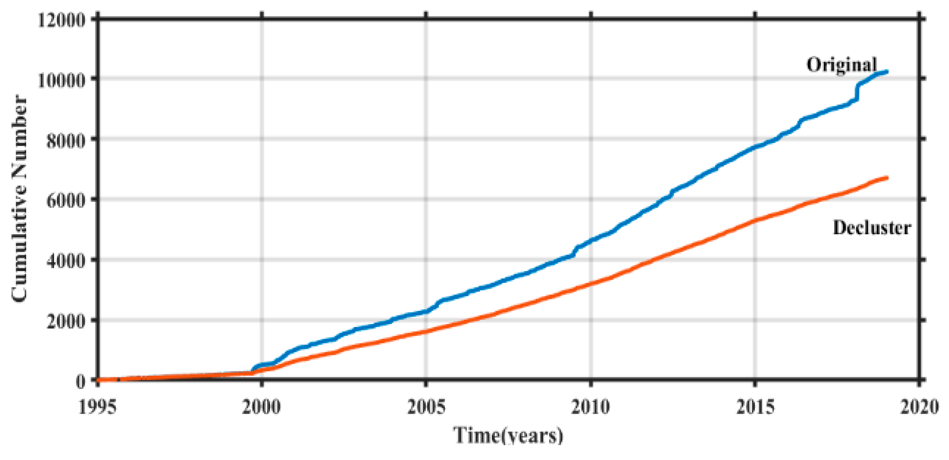
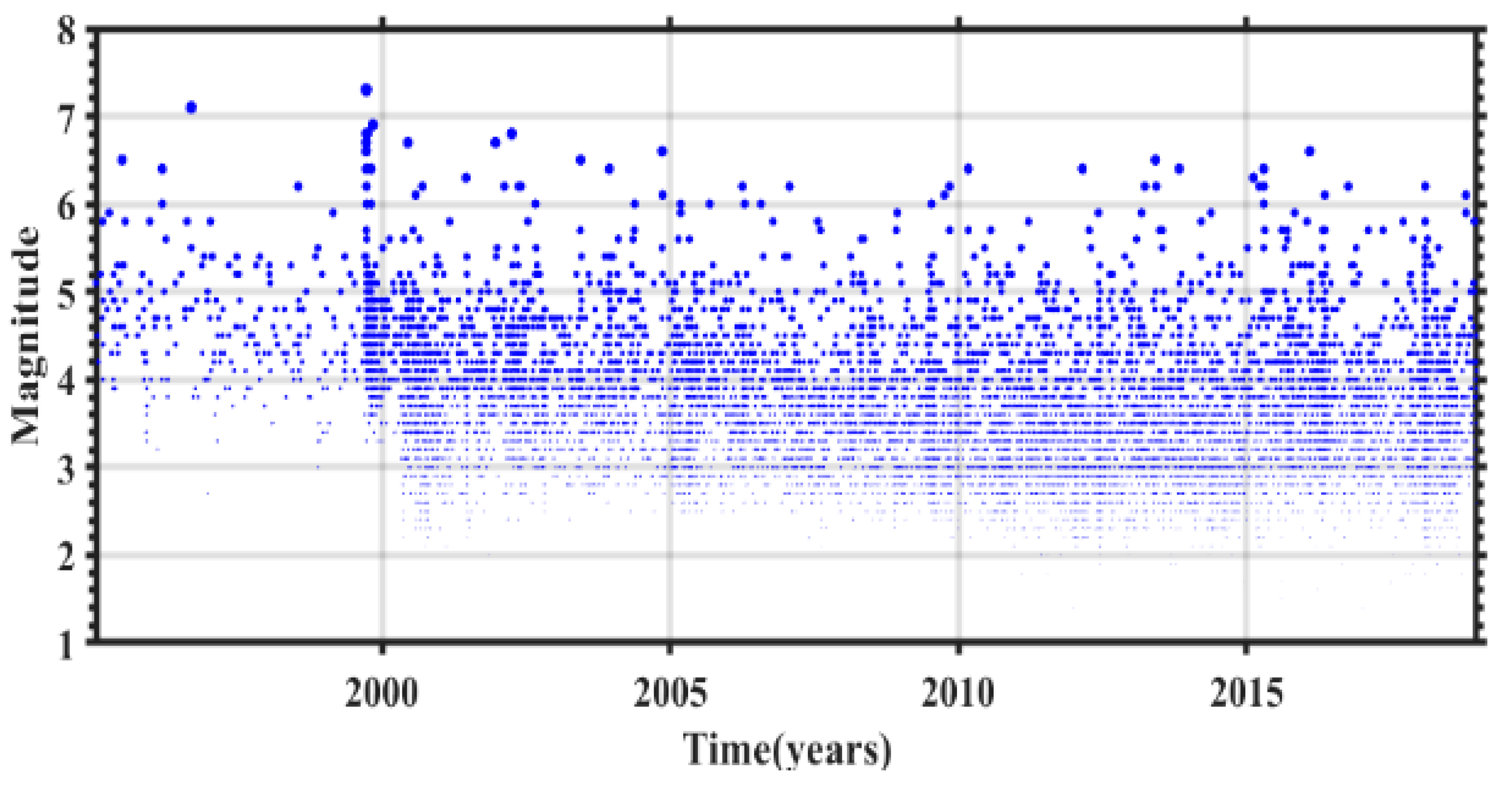
3. Earthquake Catalog
4. Method
4.1. Multifractal Methods
4.2. Estimation of b Value
5. Results
5.1. Multifractal Characteristics of the Time Distribution
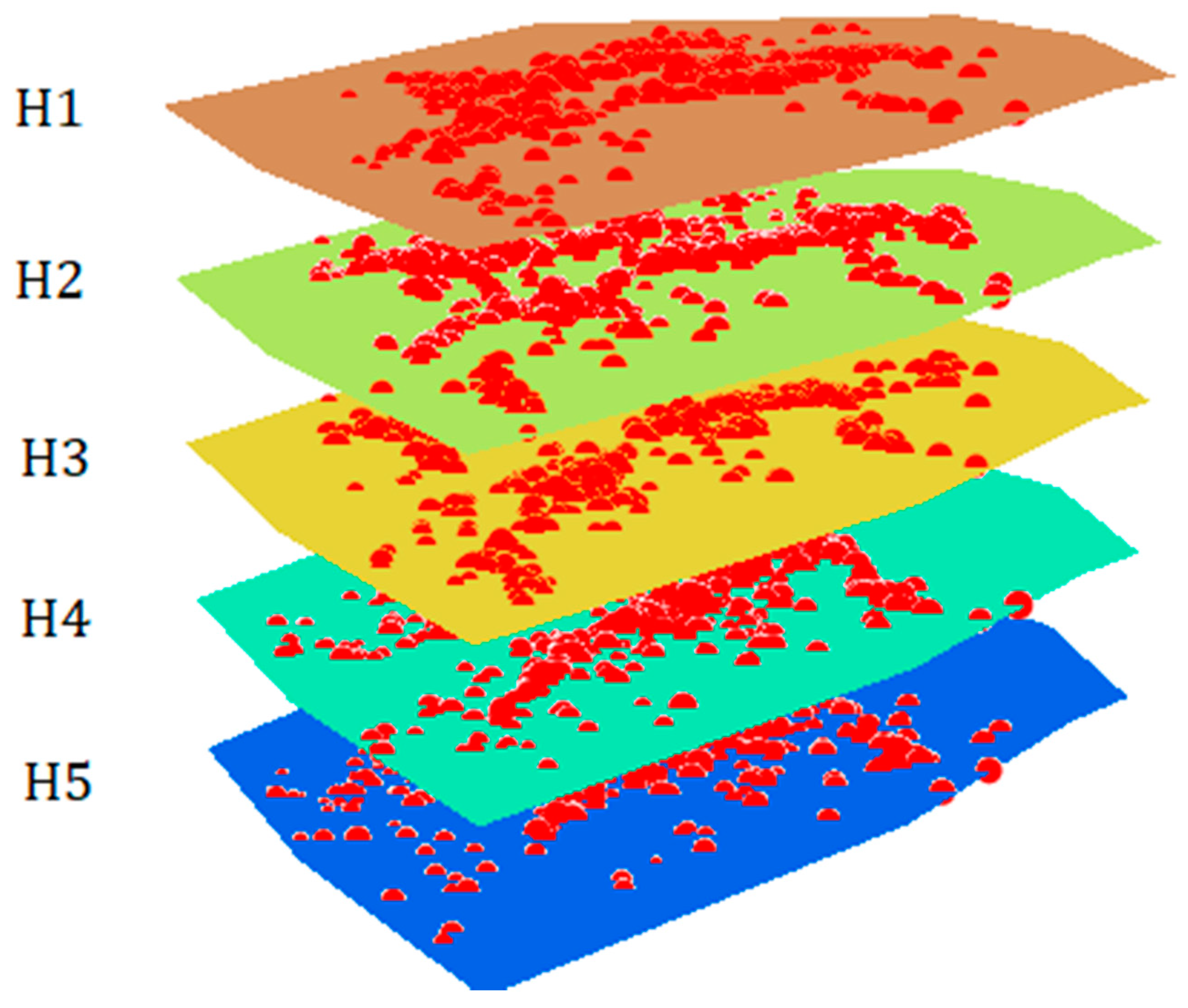
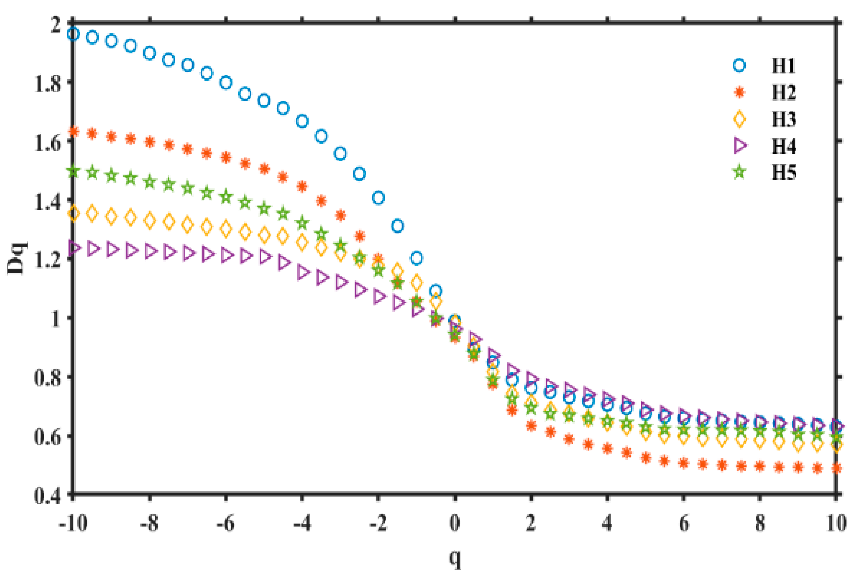
5.2. Multifractal Characteristics of the Spatial Distribution
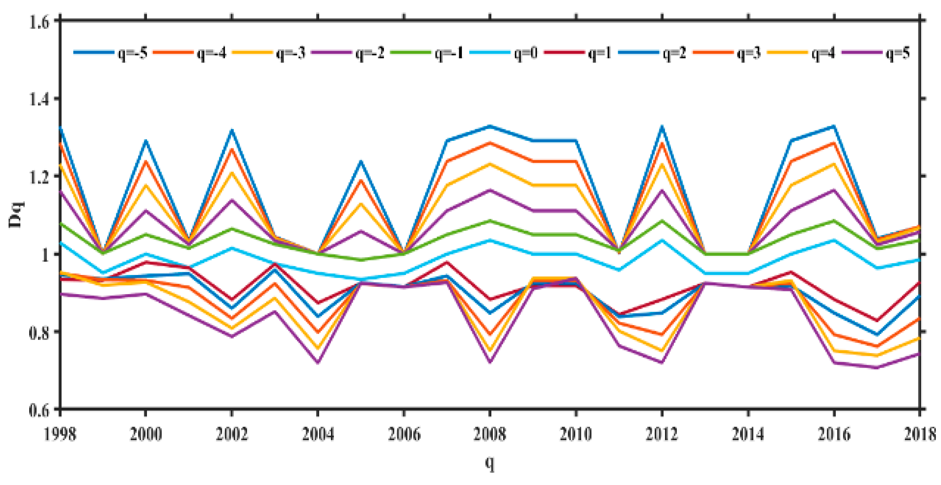
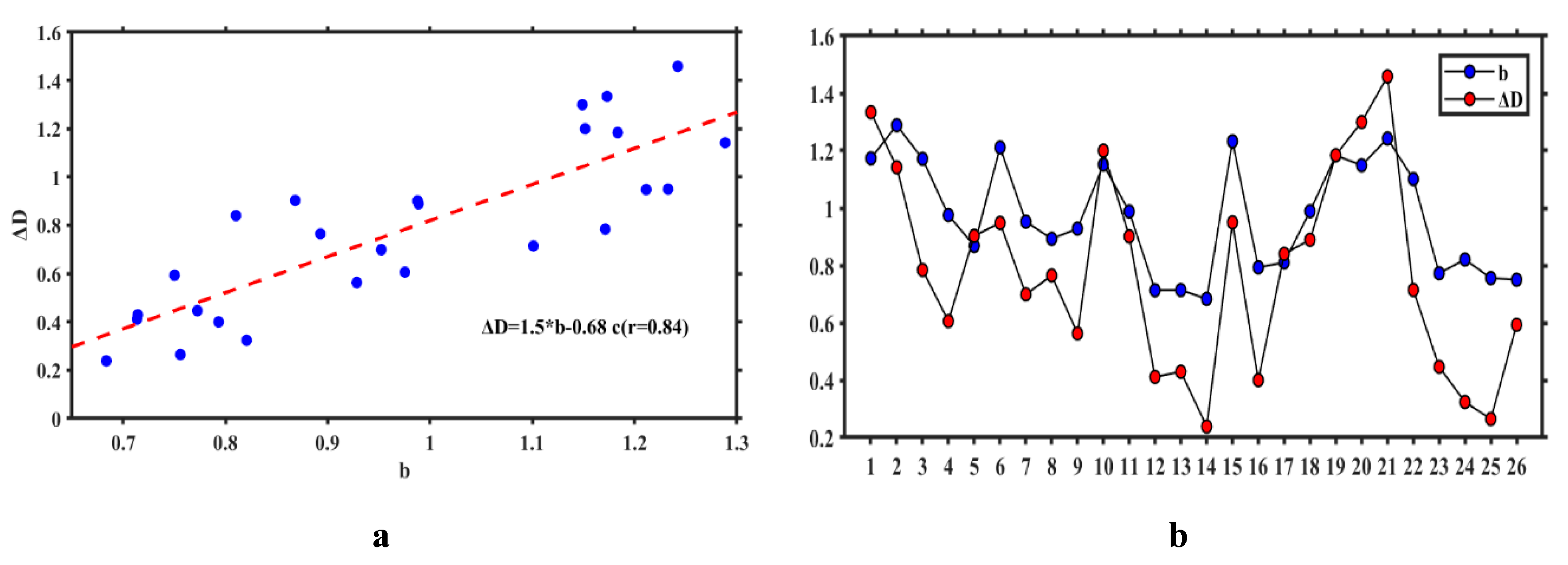
5.3. Relationship between ΔD and b Values
6. Discussion
7. Conclusions
Author Contributions
Funding
Acknowledgments
Conflicts of Interest
References
- Hirata, T. A correlation between the b-value and the fractal dimension of earthquakes. J. Geophys. Res. 1989, 94, 7507–7514. [Google Scholar] [CrossRef]
- Öncel, A.O.; Wilson, T.H. Anomalous seismicity preceding the 1999 Izmit event, NW Turkey. Geophys. J. Int. 2007, 169, 259–270. [Google Scholar] [CrossRef]
- Öztürk, S. Characteristics of seismic activity in the Western, Central and Eastern parts of the North Anatolian Fault Zone, Turkey: Temporal and spatial analysis. Acta Geophys. 2011, 59, 209–238. [Google Scholar] [CrossRef]
- Öztürk, S. A study on the correlations between seismotectonic b-value and Dc-value, and seismic quiescence Z-value in the Western Anatolian region of Turkey. Aust. J. Earth Sci. 2015, 108, 172–184. [Google Scholar] [CrossRef]
- Woessner, J.; Wiemer, S. Assessing the quality of earthquake catalogues: Estimating the magnitude of completeness and its uncertainty. Bull. Seismol. Soc. Am. 2005, 95, 684–698. [Google Scholar] [CrossRef]
- Öztürk, S. Earthquake hazard potential in the Eastern Anatolian Region of Turkey: Seismotectonic b and Dc-values and precursory quiescence Z-value. Front. Earth Sci. 2018, 12, 215–236. [Google Scholar] [CrossRef]
- Wang, J.H.; Lee, C.W. Multifractal measures of earthquakes in west Taiwan. Pure Appl. Geophys. 1996, 146, 131–145. [Google Scholar] [CrossRef]
- Chen, S.J.; David, H.; Ma, L.; Wang, L.F. Research on the multifractal characteristics of the temporal-spatial distribution of earthquakes over New Zealand area. Acta Seismol. Sin. 2003, 16, 312–322. [Google Scholar] [CrossRef]
- Pastén, D.; Muñoz, V.; Cisternas, A.; Rogan, J.; Valdivia, J.A. Monofractal and multifractal analysis of the spatial distribution of earthquakes in the central zone of Chile. Phys. Rev. E 2011, 84, 066123. [Google Scholar] [CrossRef] [PubMed]
- Balcerak, E. Seismic quiescence before the 2003 Tokachi-oki earthquake. Eos Trans. Am. Geophys. Union 2012, 93, 16. [Google Scholar] [CrossRef]
- Kagan, Y. Universality of the seismic moment-frequency relation. Pure Appl. Geophys. 1999, 155, 537–573. [Google Scholar] [CrossRef]
- Evernden, J. Study of regional seismicity and associated problems. Bull. Seismol. Soc. Am. 1970, 60, 393–446. [Google Scholar]
- Lay, T.; Wallace, T.C. Modern Global Seismology; Academic Press: Cambridge, MA, USA, 1995; p. 393. [Google Scholar]
- Schorlemmer, D.; Wiemer, S.; Wyss, M. Variations in earthquake-size distribution across different stress regimes. Nature 2005, 437, 539–542. [Google Scholar] [CrossRef] [PubMed]
- Ogata, Y.; Katsura, K. Analysis of temporal and spatial heterogeneity of magnitude frequency distribution inferred from earthquake catalogues. Geophys. J. Int. 1993, 113, 727–738. [Google Scholar] [CrossRef]
- Gulia, L.; Wiemer, S. Real-time discrimination of earthquake foreshocks and aftershocks. Nature 2019, 574, 193–199. [Google Scholar] [CrossRef] [PubMed]
- Amitrano, D. Brittle-ductile transition and associated seismicity: Experimental and numerical studies and relationship with the b value. J. Geophys. Res. Solid Earth 2003, 108, 2044–2050. [Google Scholar] [CrossRef]
- Goebel, T.H.W.; Schorlemmer, D.; Becker, T.W.; Dresen, G.; Sammis, C.G. Acoustic emissions document stress changes over many seismic cycles in stick-slip experiments. Geophys. Res. Lett. 2013, 40, 2049–2054. [Google Scholar] [CrossRef]
- Sarlis, N.V.; Skordas, E.S.; Varotsos, P.A.; Nagao, T.; Kamogawa, M.; Tanaka, H.; Uyeda, S. Minimum of the order parameter fluctuations of seismicity before major earthquakes in Japan. Proc. Natl. Acad. Sci. USA 2013, 110, 13734–13738. [Google Scholar] [CrossRef] [PubMed]
- Xie, W.Y.; Hattori, K.; Han, P. Temporal Variation and Statistical Assessment of the b Value off the Pacific Coast of Tokachi, Hokkaido, Japan. Entropy 2019, 21, 249. [Google Scholar] [CrossRef]
- Aki, K. A probabilistic synthesis of precursory phenomena. Earthq. Predict. Int. Rev. 1981, 4, 566–574. [Google Scholar]
- Wang, J.H.; Lin, W.H. A Fractal Analysis of Earthquakes in West Taiwan. Terr. Atmos. Ocean. Sci. 1993, 4, 457–462. [Google Scholar] [CrossRef]
- Legrand, D. Fractal Dimensions of Small, Intermediate, and Large Earthquakes. Bull. Seismol. Soc. Am. 2002, 92, 3318–3320. [Google Scholar] [CrossRef]
- Öncel, A.O.; Wilson, T.H. Correlation of seismotectonic variables and GPS strain measurements in western Turkey. J. Geophys. Res. Solid Earth 2004, 109, B11306. [Google Scholar]
- Wang, J.H.; Chen, K.C.; Leu, P.L.; Chang, J.H. b-Values Observations in Taiwan: A Review. Terr. Atmos. Ocean. Sci. 2015, 26, 475–492. [Google Scholar] [CrossRef]
- Mandal, P.; Rastogi, B.K. Self-organized fractal seismicity and b value of aftershocks of the 2001 Bhuj earthquake in Kutch (India). Pure Appl. Geophys. 2005, 162, 53–72. [Google Scholar] [CrossRef]
- Hattori, K. ULF geomagnetic changes associated with large earthquakes. Terr. Atmos. Ocean. Sci. 2004, 15, 329–360. [Google Scholar]
- Suppe, J. Mechanism of mountain building and metamorphism in Taiwan. Geol. Soc. China Mem. 1981, 4, 67–89. [Google Scholar]
- Hsu, Y.J.; Yu, S.B.; Simons, M.; Kuo, L.C.; Chen, H.Y. Interseismic crustal deformation in the Taiwan plate boundary zone revealed by GPS observations, seismicity, and earthquake focal mechanisms. Tectonophysics 2009, 479, 4–18. [Google Scholar] [CrossRef]
- Chan, C.H.; Hsu, Y.J.; Wu, Y.M. Possible stress states adjacent to the rupture zone of the 1999 Chi-Chi, Taiwan, earthquake. Tectonophysics 2012, 541–543, 81–88. [Google Scholar] [CrossRef]
- Wu, Y.M.; Chang, C.H.; Zhao, L.; Teng, T.L.; Nakamura, M. A comprehensive relocation of earthquakes in Taiwan from 1991 to 2005. Bull. Seismol. Soc. Am. 2008, 98, 1471–1481. [Google Scholar] [CrossRef]
- Mignan, A.; Werner, M.; Wiemer, S.; Chen, C.C.; Wu, Y.M. Bayesian estimation of the spatially varying completeness magnitude of earthquake catalogs. Bull. Seismol. Soc. Am. 2011, 101, 1371–1385. [Google Scholar] [CrossRef]
- Angelier, J.; Barrier, E.; Chu, H.T. Plate collision and paleostress trajectories in a fold-thrust belt: The foothills of Taiwan. Tectonophysics 1986, 125, 161–178. [Google Scholar] [CrossRef]
- Suppe, J.; Hu, C.T.; Chen, Y.J. Preset-day stress directions in western Taiwan inferred from borehole elongation. Pet. Geol. Taiwan 1985, 21, 1–12. [Google Scholar]
- Chang, C.P.; Chang, T.Y.; Angelier, J.; Kao, H.; Lee, J.C.; Yu, S.B. Strain and stress field in Taiwan oblique convergent system: Constraints from GPS observation and tectonic data. Earth Planet. Sci. Lett. 2003, 214, 115–127. [Google Scholar] [CrossRef]
- Yeh, Y.H.; Barrier, E.; Lin, C.H.; Angelier, J. Stress tensor analysis in the Taiwan area from focal mechanisms of earthquakes. Tectonophysics 1991, 200, 267–280. [Google Scholar]
- Wu, Y.M.; Hsu, Y.J.; Chang, C.H.; Teng, L.S.; Nakamura, M. Temporal and spatial variation of stress field in Taiwan from 1991 to 2007: Insights from comprehensive first motion focal mechanism catalog. Earth Planet. Sci. Lett. 2010, 298, 306–316. [Google Scholar] [CrossRef]
- Chen, H.Y.; Kuo, L.C.; Yu, S.B. Coseismic movement and seismic ground motion associated with the 31 March 2002 Hualien “331” earthquake. Terr. Atmos. Oceans Sci. 2004, 15, 683–695. [Google Scholar] [CrossRef][Green Version]
- Hu, J.C.; Cheng, L.W.; Chen, H.Y.; Wu, Y.M.; Lee, J.C.; Chen, Y.G.; Lin, K.C.; Rau, R.J.; Kuochen, H.; Chen, H.H.; et al. Coseismic deformation revealed by inversion of strong motion and GPS data: The 2003 Chengkung earthquake in Taiwan. Geophys. J. Int. 2007, 169, 667–674. [Google Scholar] [CrossRef]
- Wu, Y.M.; Chang, C.H.; Zhao, L.; Hsiao, N.C.; Chen, Y.G.; Hsu, S.K. Relocation of the 2006 Pingtung earthquake sequence and seismotectonics in Southern Taiwan. Tectonophysics 2009, 479, 19–27. [Google Scholar] [CrossRef]
- Cao, A.; Gao, S.S. Temporal variation of seismic b-values beneath northeastern Japan island arc. Geophys. Res. Lett. 2002, 29, 48-1–48-3. [Google Scholar] [CrossRef]
- Wiemer, S.; Wyss, M. Minimum magnitude of completeness in earthquake catalogs: Examples from Alaska, the western United States, and Japan. Bull. Seismol. Soc. Am. 2000, 90, 859–869. [Google Scholar] [CrossRef]
- Chan, C.H.; Wu, Y.M.; Tseng, T.L.; Lin, T.L.; Chen, C.C. Spatial and temporal evolution of b-values before large earthquakes in Taiwan. Tectonophysics 2012, 532, 215–222. [Google Scholar] [CrossRef]
- Wang, J.H. Depth distribution of shallow earthquakes in Taiwan. J. Geol. Soc. China. 1994, 37, 125–142. [Google Scholar]
- Sunmonu, L.A.; Dimri, V.P.; Prakash, M.R.; Bansal, A.R. Multifractal approach to the time series of m ≥ 7.0 earthquake in himalayan region and its vicinity during 1895–1995. J. Geol. Soc. India 2001, 58, 163–169. [Google Scholar]
- Gutenberg, B.; Richter, C.F. Earthquake magnitude, intensity, energy, and acceleration. Bull. Seismol. Soc. Am. 1942, 32, 163–191. [Google Scholar]
- Noh, M. A parametric estimation of Richter-b and m max from an earthquake catalog. Geosci. J. 2014, 18, 339–345. [Google Scholar] [CrossRef]
- Aki, K. Maximum likelihood estimate of b in the formula logN = a − bM and its confidence limits. Bull. Earthq. Res. Inst. Tokyo Univ. 1965, 43, 237–239. [Google Scholar]
- A method for determining the value of b in a formula logN = a − bM showing the magnitude frequency relation for earthquakes. Geophys. Bull. Hokkaido Univ. 1965, 13, 99–103.
- Yin, L.R.; Li, X.L.; Zheng, W.F.; Yin, Z.; Song, L.H.; Ge, L.J.; Zeng, Q. Fractal dimension analysis for seismicity spatial and temporal distribution in the circum-Pacific seismic belt. J. Earth Syst. Sci. 2019, 128, 22. [Google Scholar] [CrossRef]
- Márquez-Rámirez, V.H.; Pichardo, F.A.N.; Reyes-Dávila, G. Multifractality in seismicity spatial distributions: Significance and possible precursory applications as found for two cases in different tectonic environments. Pure Appl. Geophys. 2012, 169, 2091–2105. [Google Scholar] [CrossRef]
- Singh, C.; Singh, A.; Chadha, R. Fractal and b-value mapping in Eastern Himalaya and Southern Tibet. Bull. Seismol. Soc. Am. 2009, 99, 3529–3533. [Google Scholar] [CrossRef]
- Öncel, A.O.; Alptekin, Ö.; Main, I.G. Temporal variations of the fractal properties of seismicity in the western part of the North Anatolian fault zone: Possible artifacts due to improvements in station coverage. Nonlinear Process. Geophys. 1995, 2, 147–157. [Google Scholar] [CrossRef]
- De Rubeis, V.; Dimitriu, P.; Papadimitriou, E.; Tosi, P. Recurrent patterns in the spatial behaviour of Italian seismicity revealed by the fractal approach. Geophys. Res. Lett. 1993, 20, 1911–1914. [Google Scholar] [CrossRef]
- Zhu, L.R.; Zhou, S.Y.; Yang, M.L.; Hong, S.Z.; Gong, Y.Q.; Wang, H.T. The Precision Estimate of Multi-Fractal Methods of Time Sequence of Earthquakes. Earthq. Res. China 2000, 14, 47–56. [Google Scholar]
- Varotsos, P.A.; Sarlis, N.V.; Skordas, E.S. Order parameter fluctuations in natural time and b-value variation before large earthquakes. Nat. Hazards Earth Syst. Sci. 2012, 12, 3473–3481. [Google Scholar] [CrossRef]
- Shi, H.; Meng, L.; Zhang, X.; Chang, Y.; Yang, Z.; Xie, W.; Hattori, K.; Han, P. Decrease in b value prior to the Wenchuan earthquake (M (s) 8.0). Chin. J. Geophys. 2018, 61, 1874–1882. [Google Scholar]
- Gulia, L.; Wiemer, S. The influence of tectonic regimes on the earthquake size distribution: A case study for Italy. Geophys. Res. Lett. 2010, 37, L10305. [Google Scholar] [CrossRef]
- Scholz, C.H. The frequency magnitude relation of microfracturing in rock and its relation to earthquakes. Bull. Seismol. Soc. Am. 1968, 58, 399–415. [Google Scholar]
- Spada, M.; Tormann, T.; Wiemer, S.; Enescu, B. Generic dependence of the frequency-size distribution of earthquakes on depth and its relation to the strength profile of the crust. Geophys. Res. Lett. 2013, 40, 709–714. [Google Scholar] [CrossRef]
- Wiemer, S.; Wyss, M. Mapping the frequency-magnitude distribution in asperities: An improved technique to calculate recurrence times? J. Geophys. Res. Solid Earth 1997, 102, 15115–15128. [Google Scholar] [CrossRef]
- Grassberger, P.; Procaccia, I. Measuring the strangeness of strange attractors. Phys. D Nonlinear Phenom. 1983, 9, 189–208. [Google Scholar] [CrossRef]
- Khan, P. Mapping of b-value beneath the Shillong Plateau. Gondwana Res. 2005, 8, 271–276. [Google Scholar] [CrossRef]
- Pailoplee, S.; Choowong, M. Earthquake frequency-magnitude distribution and fractal dimension in mainland Southeast Asia. Earth Planets Space 2014, 66, 8. [Google Scholar] [CrossRef]


| Depth | ΔD | b |
|---|---|---|
| H1 | 1.33 | 1.17 ± 0.01 |
| H2 | 1.14 | 1.29 ± 0.01 |
| H3 | 0.78 | 1.17 ± 0.02 |
| H4 | 0.61 | 0.98 ± 0.02 |
| H5 | 0.90 | 0.87 ± 0.02 |
© 2020 by the authors. Licensee MDPI, Basel, Switzerland. This article is an open access article distributed under the terms and conditions of the Creative Commons Attribution (CC BY) license (http://creativecommons.org/licenses/by/4.0/).
Share and Cite
Hui, C.; Cheng, C.; Ning, L.; Yang, J. Multifractal Characteristics of Seismogenic Systems and b Values in the Taiwan Seismic Region. ISPRS Int. J. Geo-Inf. 2020, 9, 384. https://doi.org/10.3390/ijgi9060384
Hui C, Cheng C, Ning L, Yang J. Multifractal Characteristics of Seismogenic Systems and b Values in the Taiwan Seismic Region. ISPRS International Journal of Geo-Information. 2020; 9(6):384. https://doi.org/10.3390/ijgi9060384
Chicago/Turabian StyleHui, Chun, Changxiu Cheng, Lixin Ning, and Jing Yang. 2020. "Multifractal Characteristics of Seismogenic Systems and b Values in the Taiwan Seismic Region" ISPRS International Journal of Geo-Information 9, no. 6: 384. https://doi.org/10.3390/ijgi9060384
APA StyleHui, C., Cheng, C., Ning, L., & Yang, J. (2020). Multifractal Characteristics of Seismogenic Systems and b Values in the Taiwan Seismic Region. ISPRS International Journal of Geo-Information, 9(6), 384. https://doi.org/10.3390/ijgi9060384