Spatial Analysis of Housing Prices and Market Activity with the Geographically Weighted Regression


Abstract
1. Introduction
2. Literature Review
3. Methods of Research
3.1. Geographically Weighted Regression (GWR)
3.2. Mixed Geographically Weighted Regression (MGWR)
- Step 1. Supply an initial value for , say , using OLS (ordinary least squares)
- Step 2. Set i = 1
- Step 3. Set
- Step 4. Set
- Step 5. Set i = i + 1
- Step 6. Return to Step 3, unless converges to
4. General Data Characteristics
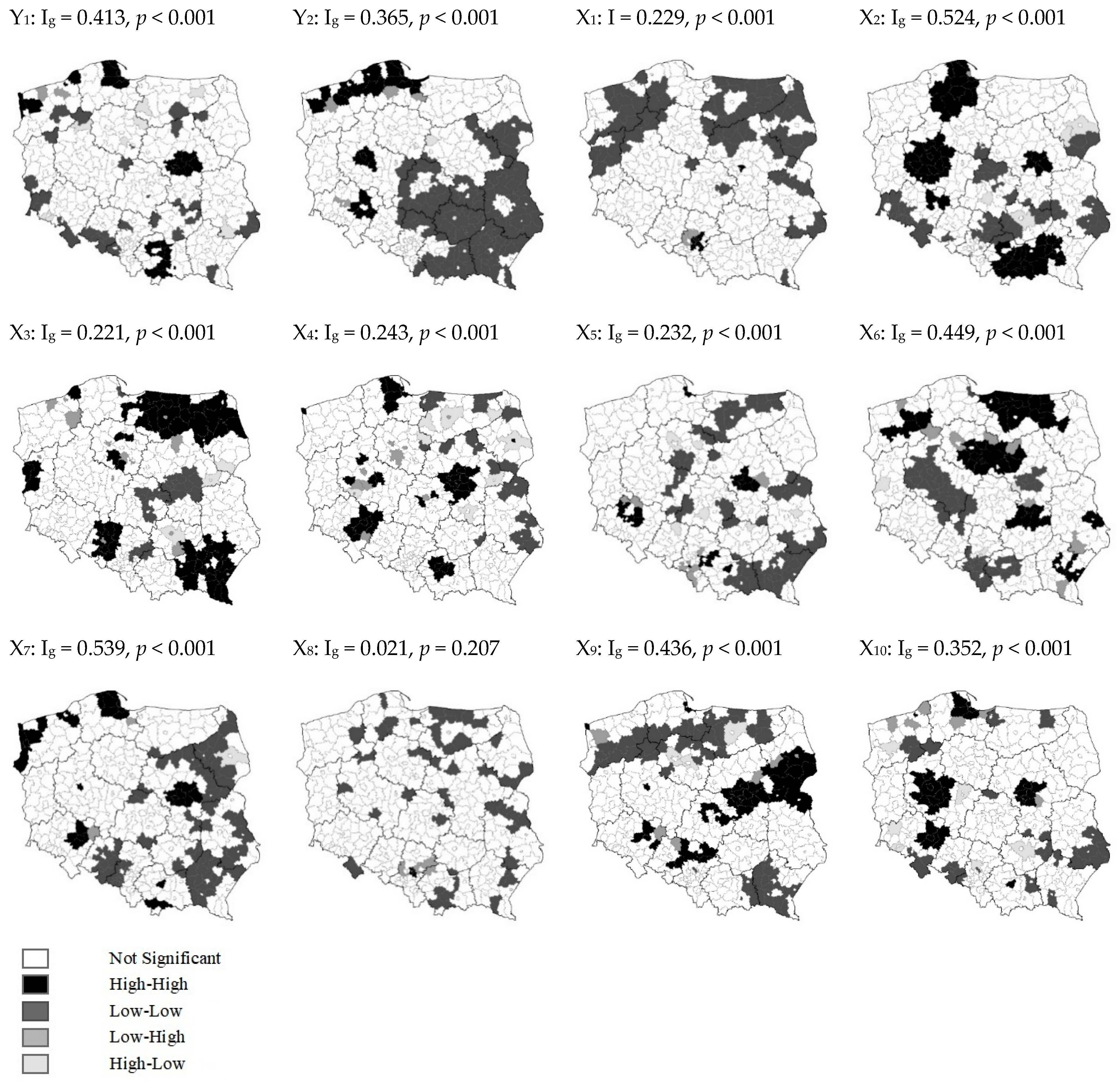
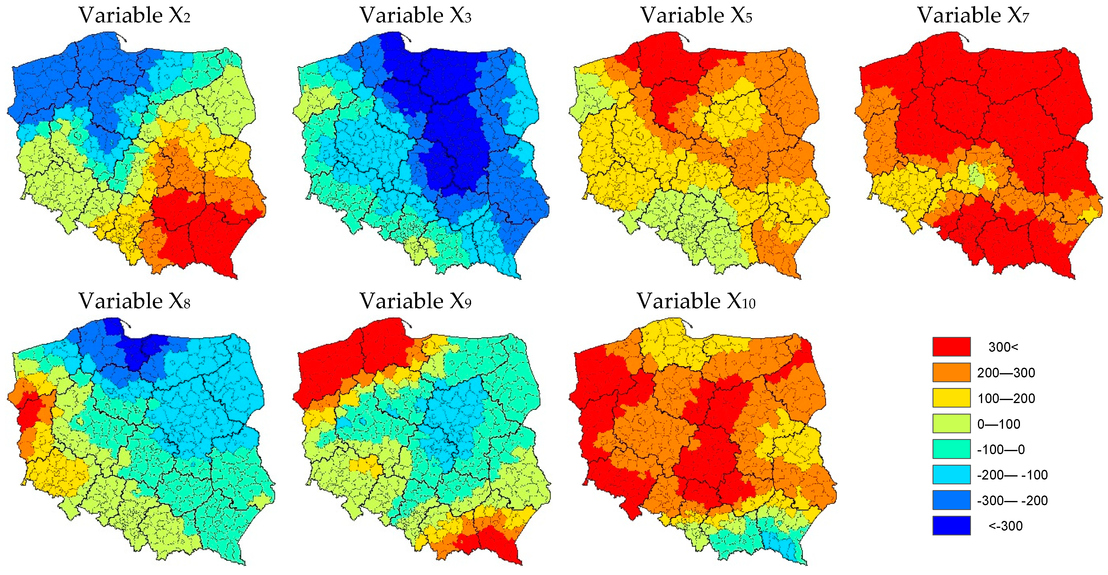
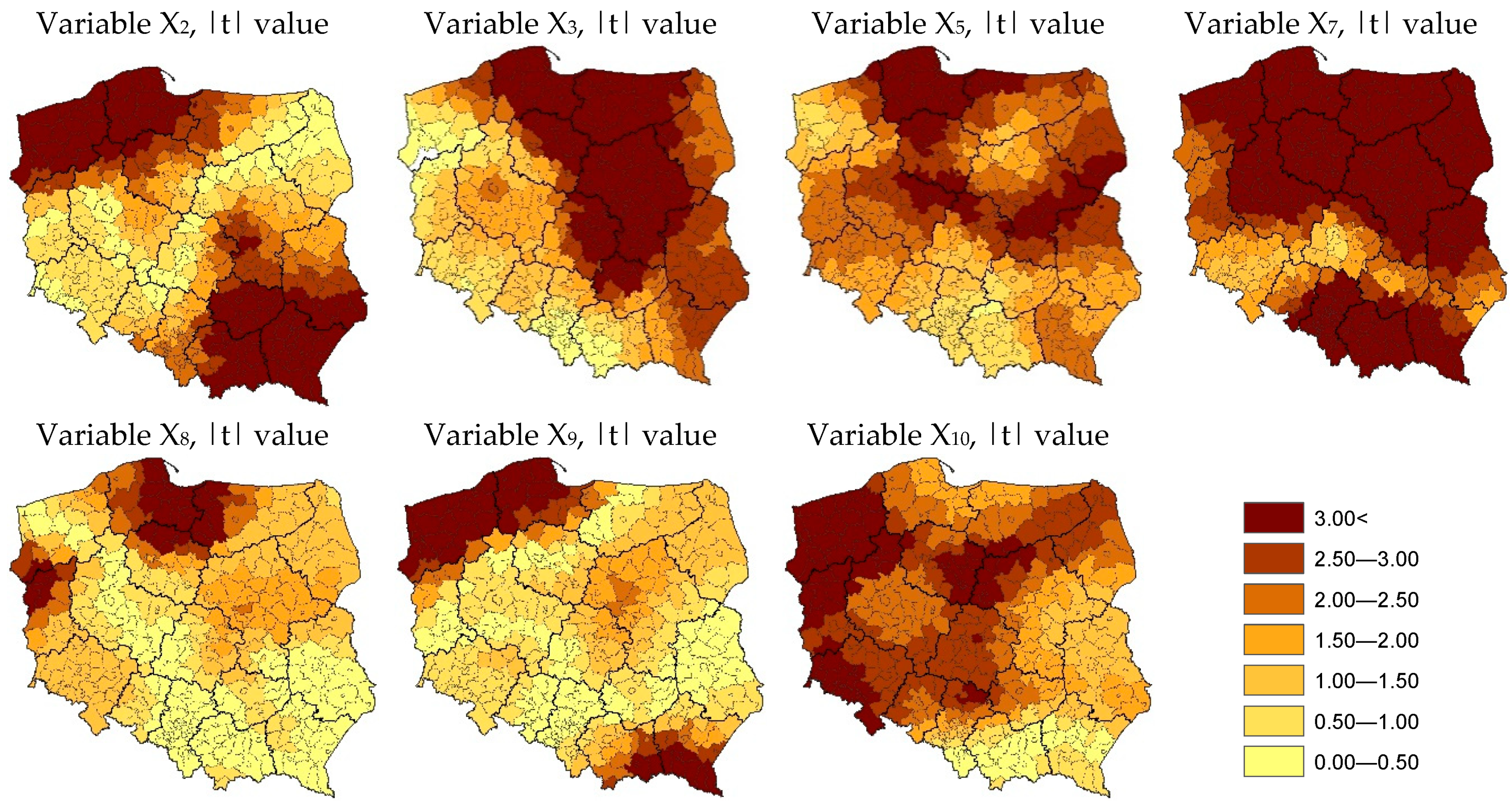
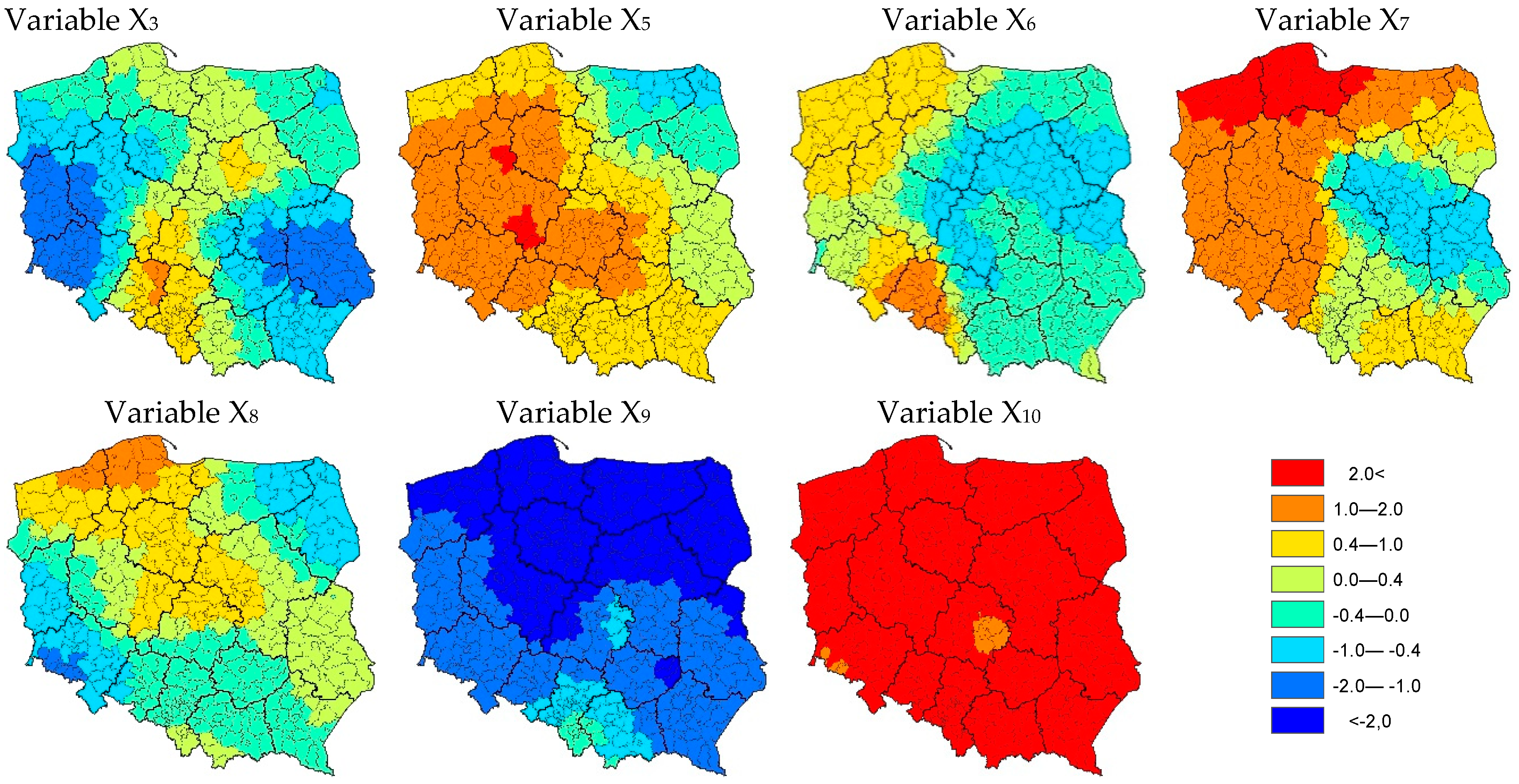
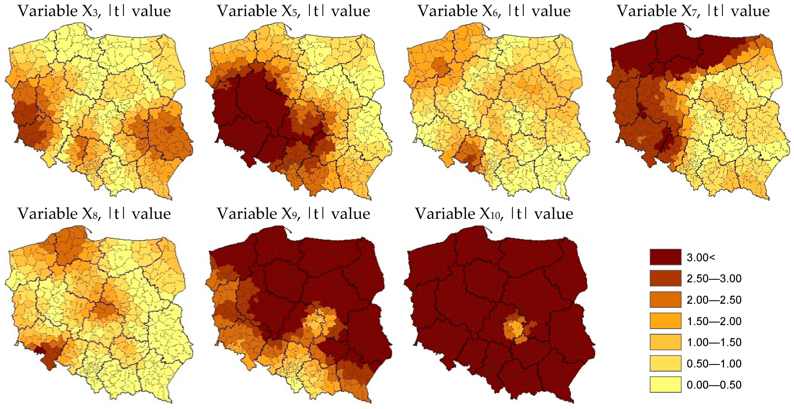
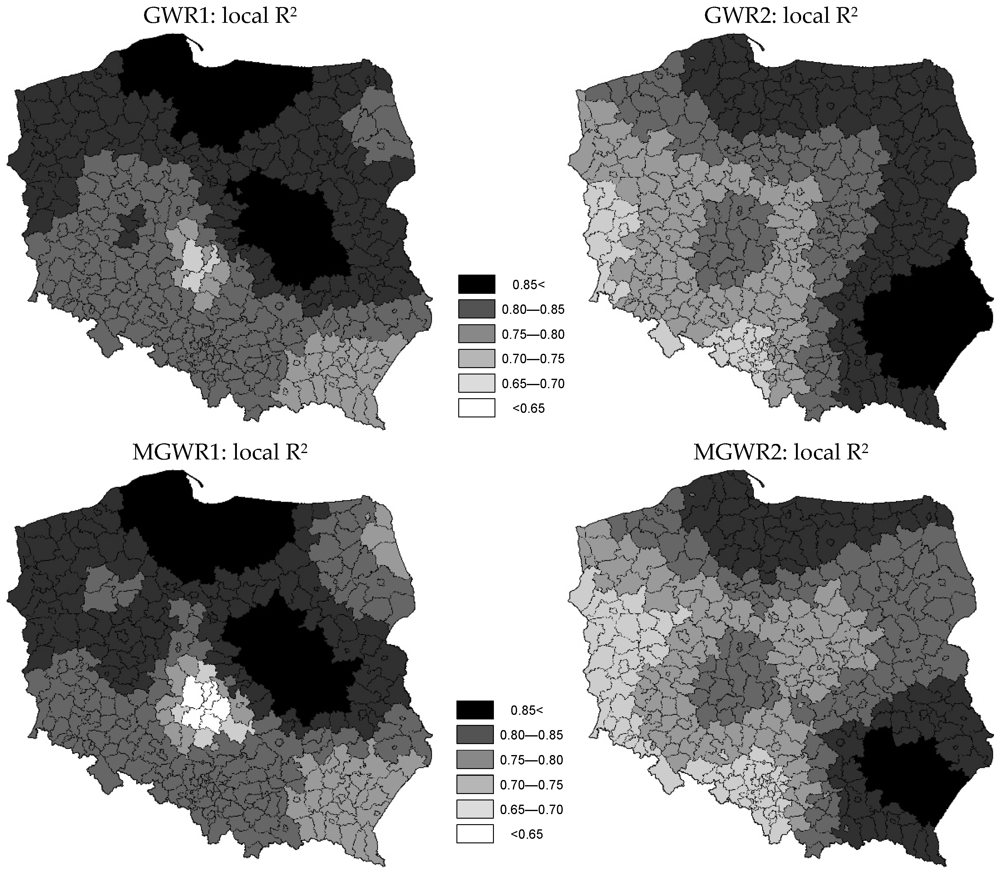
5. Results and Discussion
6. Summary and Conclusions
Author Contributions
Funding
Conflicts of Interest
References
- Adams, Z.; Füss, R. Macroeconomic Determinants of International Housing Markets. J. Hous. Econ. 2010, 19, 38–50. [Google Scholar] [CrossRef]
- Hott, C.; Monnin, P. Fundamental Real Estate Prices: An Empirical Estimation with International Data. J. Real Estate Financ. Econ. 2008, 36, 427–450. [Google Scholar] [CrossRef]
- Gasparėnienė, L.; Remeikienė, R.; Skuka, A. Assessment of the Impact of Macroeconomic Factors on Housing Price Level: Lithuanian Case. Intellect. Econ. 2016, 10, 122–127. [Google Scholar] [CrossRef]
- Lee, C.L. Housing Price Volatility and Its Determinants. Int. J. Hous. Mark. Anal. 2009, 2, 293–308. [Google Scholar] [CrossRef]
- Anas, A.; Eum, S.J. Hedonic Analysis of a Housing Market in Disequilibrium. J. Urban Econ. 1984, 15, 87–106. [Google Scholar] [CrossRef]
- DeSilva, S.; Elmelech, Y. Housing Inequality in the United States: Explaining the White-Minority Disparities in Homeownership. Hous. Stud. 2012, 27, 1–26. [Google Scholar] [CrossRef]
- Engelhardt, G.V.; Poterba, J.M. House Prices and Demographic Change: Canadian Evidence. Reg. Sci. Urban Econ. 1991, 21, 539–546. [Google Scholar] [CrossRef]
- Essafi, Y.; Simon, A. Housing Market and Demography, Evidence from French Panel Data. Eur. Real Estate Soc. 2015, 2015, 107–133. [Google Scholar] [CrossRef]
- Lin, W.-S.; Tou, J.-C.; Lin, S.-Y.; Yeh, M.-Y. Effects of Socioeconomic Factors on Regional Housing Prices in the USA. Int. J. Hous. Mark. Anal. 2014, 7, 30–41. [Google Scholar] [CrossRef]
- Magnusson, L.; Turner, B. Countryside Abandoned? Suburbanization and Mobility in Sweden. Eur. J. Hous. Policy 2003, 3, 35–60. [Google Scholar] [CrossRef]
- Gallin, J. The Long-run Relationship between House Prices and Income: Evidence from Local Housing Markets. Real Estate Econ. 2006, 34, 417–438. [Google Scholar] [CrossRef]
- Jud, G.D.; Winkler, D.T. The Dynamics of Metropolitan Housing Prices. J. Real Estate Res. 2002, 23, 29–46. [Google Scholar]
- Reichert, A.K. The Impact of Interest Rates, Income, and Employment upon Regional Housing Prices. J. Real Estate Financ. Econ. 1990, 3, 373–391. [Google Scholar] [CrossRef]
- Berg, L. Prices on the Second-Hand Market for Swedish Family Houses: Correlation, Causation and Determinants. Eur. J. Hous. Policy 2002, 2, 1–24. [Google Scholar] [CrossRef]
- De Bruyne, K.; Van Hove, J. Explaining the Spatial Variation in Housing Prices: An Economic Geography Approach. Appl. Econ. 2013, 45, 1673–1689. [Google Scholar] [CrossRef]
- Allen, J.; Amano, R.; Byrne, D.P.; Gregory, A.W. Canadian City Housing Prices and Urban Market Segmentation. Can. J. Econ. Can. Déconomique 2009, 42, 1132–1149. Available online: https://www.jstor.org/stable/40389501 (accessed on 20 March 2020). [CrossRef]
- Ridker, R.G.; Henning, J.A. The Determinants of Residential Property Values with Special Reference to Air Pollution. Rev. Econ. Stat. 1967, 49, 246–257. [Google Scholar] [CrossRef]
- Kim, C.W.; Phipps, T.T.; Anselin, L. Measuring the Benefits of Air Quality Improvement: A Spatial Hedonic Approach. J. Environ. Econ. Manag. 2003, 45, 24–39. [Google Scholar] [CrossRef]
- Saphores, J.-D.; Aguilar-Benitez, I. Smelly Local Polluters and Residential Property Values: A Hedonic Analysis of Four Orange County (California) Cities. Estud. Econ. 2005, 20, 197–218. Available online: https://www.jstor.org/stable/40311503 (accessed on 25 March 2020).
- Orenstein, D.E.; Hamburg, S.P. Population and Pavement: Population Growth and Land Development in Israel. Popul. Environ. 2010, 31, 223–254. [Google Scholar] [CrossRef]
- Broitman, D.; Koomen, E. Regional Diversity in Residential Development: A Decade of Urban and Peri-Urban Housing Dynamics in The Netherlands. Lett. Spat. Resour. Sci. 2015, 8, 201–217. [Google Scholar] [CrossRef]
- Belke, A.; Keil, J. Fundamental Determinants of Real Estate Prices: A Panel Study of German Regions. Int. Adv. Econ. Res. 2018, 24, 25–45. [Google Scholar] [CrossRef]
- Grum, B.; Govekar, D.K. Influence of Macroeconomic Factors on Prices of Real Estate in Various Cultural Environments: Case of Slovenia, Greece, France, Poland and Norway. Procedia Econ. Financ. 2016, 39, 597–604. [Google Scholar] [CrossRef]
- Fujita, M.; Krugman, P.R.; Venables, A. The Spatial Economy: Cities, Regions, and International Trade; MIT press: Cambridge, MA, USA, 1999. [Google Scholar]
- Gaspareniene, L.; Venclauskiene, D.; Remeikiene, R. Critical Review of Selected Housing Market Models Concerning the Factors That Make Influence on Housing Price Level Formation in the Countries with Transition Economy. Procedia-Soc. Behav. Sci. 2014, 110, 419–427. [Google Scholar] [CrossRef]
- Holly, S.; Pesaran, M.H.; Yamagata, T. A Spatio-Temporal Model of House Prices in the USA. J. Econ. 2010, 158, 160–173. [Google Scholar] [CrossRef]
- Lee, L.; Yu, J. Some Recent Developments in Spatial Panel Data Models. Reg. Sci. Urban Econ. 2010, 40, 255–271. [Google Scholar] [CrossRef]
- Otto, P.; Schmid, W. Spatiotemporal Analysis of German Real-Estate Prices. Ann. Reg. Sci. 2018, 60, 41–72. [Google Scholar] [CrossRef]
- Griffith, D.A. Modeling Spatial Autocorrelation in Spatial Interaction Data: Empirical Evidence from 2002 Germany Journey-to-Work Flows. J. Geogr. Syst. 2009, 11, 117–140. [Google Scholar] [CrossRef]
- Griffith, D.A. Spatial Filtering. In Handbook of Applied Spatial Analysis; Fisher, M.M., Getis, A., Eds.; Springer: Berlin, Germany, 2010. [Google Scholar]
- Tiefelsdorf, M.; Griffith, D.A. Semiparametric Filtering of Spatial Autocorrelation: The Eigenvector Approach. Environ. Plan. Econ. Space 2007, 39, 1193–1221. [Google Scholar] [CrossRef]
- Thayn, J.B.; Simanis, J.M. Accounting for Spatial Autocorrelation in Linear Regression Models Using Spatial Filtering with Eigenvectors. Ann. Assoc. Am. Geogr. 2013, 103, 47–66. [Google Scholar] [CrossRef]
- Griffith, D.A. Spatial-Filtering-Based Contributions to a Critique of Geographically Weighted Regression (GWR). Environ. Plan. A 2008, 40. [Google Scholar] [CrossRef]
- Huang, B.; Wu, B.; Barry, M. Geographically and Temporally Weighted Regression for Modeling Spatio-Temporal Variation in House Prices. Int. J. Geogr. Inf. Sci. 2010, 24, 383–401. [Google Scholar] [CrossRef]
- Lu, B.; Charlton, M.; Fotheringhama, A.S. Geographically Weighted Regression Using a Non-Euclidean Distance Metric with a Study on London House Price Data. Procedia Environ. Sci. 2011, 7, 92–97. [Google Scholar] [CrossRef]
- Kestens, Y.; Thériault, M.; Des Rosiers, F. Heterogeneity in Hedonic Modelling of House Prices: Looking at Buyers’ Household Profiles. J. Geogr. Syst. 2006, 8, 61–96. [Google Scholar] [CrossRef]
- Yu, D. Modeling Owner-Occupied Single-Family House Values in the City of Milwaukee: A Geographically Weighted Regression Approach. GIScience Remote Sens. 2007, 44, 267–282. [Google Scholar] [CrossRef]
- McCord, M.; Davis, P.T.; Haran, M.; McGreal, S.; McIlhatton, D. Spatial Variation as a Determinant of House Price. J. Financ. Manag. Prop. Constr. 2012, 17, 49–72. [Google Scholar] [CrossRef]
- Yang, J.; Bao, Y.; Zhang, Y.; Li, X.; Ge, Q. Impact of Accessibility on Housing Prices in Dalian City of China Based on a Geographically Weighted Regression Model. Chin. Geogr. Sci. 2018, 28, 505–515. [Google Scholar] [CrossRef]
- Helbich, M.; Brunauer, W.; Vaz, E.; Nijkamp, P. Spatial Heterogeneity in Hedonic House Price Models: The Case of Austria. Urban Stud. 2014, 51, 390–411. [Google Scholar] [CrossRef]
- Mondal, B.; Das, D.N.; Dolui, G. Modeling Spatial Variation of Explanatory Factors of Urban Expansion of Kolkata: A Geographically Weighted Regression Approach. Model. Earth Syst. Environ. 2015, 1, 29. [Google Scholar] [CrossRef]
- Sholihin, M.; Soleh, A.M.; Djuraidah, A. Geographically and Temporally Weighted Regression (GTWR) for Modeling Economic Growth Using R. Int. J. Comput. Sci. Netw. 2017, 6, 800–805. [Google Scholar]
- Wu, C.; Ren, F.; Hu, W.; Du, Q. Multiscale Geographically and Temporally Weighted Regression: Exploring the Spatiotemporal Determinants of Housing Prices. Int. J. Geogr. Inf. Sci. 2019, 33, 489–511. [Google Scholar] [CrossRef]
- Purhadi, P.; Yasin, H. Mixed Geographically Weighted Regression Model (Case Study: The Percentage of Poor Households in Mojokerto 2008. Eur. J. Sci. Res. 2012, 69, 188–196. [Google Scholar]
- Rencher, A.C.; Schaalje, G.B. Linear Models in Statistics; John Wiley & Sons: Hoboken, NJ, USA, 2008. [Google Scholar]
- Fotheringham, A.S.; Brunsdon, C.; Charlton, M. Geographically Weighted Regression: The Analysis of Spatially Varying Relationships; John Wiley & Sons: Hoboken, NJ, USA, 2003. [Google Scholar]
- Mei, C.-L.; Wang, N.; Zhang, W.-X. Testing the Importance of the Explanatory Variables in a Mixed Geographically Weighted Regression Model. Environ. Plan. A 2006, 38, 587–598. [Google Scholar] [CrossRef]
- Brunsdon, C.; Fotheringham, S.; Charlton, M. Geographically Weighted Regression as a Statistical Model; Working paper, Spatial Analysis Research Group; Department of Geography, University of Newcastle-upon-Tyne: Newcastle, UK, 2000. [Google Scholar]
- Akaike, H. Information Theory and an Extension of the Maximum Likelihood Principle. In Selected Papers of Hirotugu Akaike; Springer: Berlin/Heidelberg, Germany, 1998; pp. 199–213. [Google Scholar]
- Hurvich, C.M.; Simonoff, J.S.; Tsai, C.-L. Smoothing Parameter Selection in Nonparametric Regression Using an Improved Akaike Information Criterion. J. R. Stat. Soc. Ser. B Stat. Methodol. 1998, 60, 271–293. [Google Scholar] [CrossRef]
- Leung, Y.; Mei, C.-L.; Zhang, W.-X. Statistical Tests for Spatial Nonstationarity Based on the Geographically Weighted Regression Model. Environ. Plan. A 2000, 32, 9–32. [Google Scholar] [CrossRef]
- LeSage, J.P. A Family of Geographically Weighted Regression Models. In Advances in Spatial Econometrics; Springer: Berlin, Germany, 2004; pp. 241–264. [Google Scholar]
- Wheeler, D.C.; Páez, A. Geographically Weighted Regression. In Advances in Spatial Econometrics; Anselin, L.R., Florax, J.G.M., Rey, S.J., Eds.; Springer: Heidelberg, Germany, 2010. [Google Scholar]
- Lu, B.; Harris, P.; Charlton, M.; Brunsdon, C. The GWmodel R Package: Further Topics for Exploring Spatial Heterogeneity Using Geographically Weighted Models. Geo-Spat. Inf. Sci. 2014, 17, 85–101. [Google Scholar] [CrossRef]
- Ispriyanti, D.; Yasin, H.; Warsito, B.; Hoyyi, A.; Winarso, K. Mixed Geographically Weighted Regression Using Adaptive Bandwidth to Modeling of Air Polluter Standard Index. ARPN J. Eng. Appl. Sci. 2017, 12, 4477–4482. [Google Scholar] [CrossRef]
- Speckman, P. Kernel Smoothing in Partial Linear Models. J. R. Stat. Soc. Ser. B Methodol. 1988, 50, 413–436. [Google Scholar] [CrossRef]
- Wei, C.-H.; Qi, F. On the Estimation and Testing of Mixed Geographically Weighted Regression Models. Econ. Model. 2012, 29, 2615–2620. [Google Scholar] [CrossRef]
- Lewandowska-Gwarda, K. Geographically Weighted Regression in the Analysis of Unemployment in Poland. ISPRS Int. J. Geo-Inf. 2018, 7, 17. [Google Scholar] [CrossRef]
- Foryś, I. Społeczno-Gospodarcze Determinanty Rozwoju Rynku Mieszkaniowego w Polsce: Ujęcie Ilościowe. Wydawnictwo Naukowe Uniwersytetu Szczecińskiego 2011, 793, 398. [Google Scholar]
- Rącka, I.; Rehman, S.K. Housing Market in Capital Cities–the Case of Poland and Portugal. Geomat. Environ. Eng. 2018, 12, 75–87. [Google Scholar] [CrossRef]
- Sitek, M. Situation in the Polish Housing Market Compared to Other EU Countries. J. Int. Stud. 2014, 7, 57–69. [Google Scholar] [CrossRef]
- Tomal, M. The Impact of Macro Factors on Apartment Prices in Polish Counties: A Two-Stage Quantile Spatial Regression Approach. Real Estate Manag. Valuat. 2019, 27, 1–14. [Google Scholar] [CrossRef]
- Cliff, A.D. Spatial Autocorrelation; Pion.: London, UK, 1973. [Google Scholar]
- Goodchild, M.F.; Janelle, D.G. Spatially Integrated Social Science; Oxford University Press: Oxford, UK, 2004. [Google Scholar]


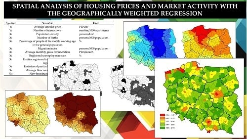
| Symbol | Variable | Unit |
|---|---|---|
| Y1 | Average unit flat price | PLN/m2 (New Polish Zloty/m2) |
| Y2 | Number of transactions | number/1000 apartments |
| X1 | Population density | persons/km2 |
| X2 | Number of births | persons/1000 population |
| X3 | Percentage of people of the mobile working age in the general population | % |
| X4 | Migration index | persons/1000 population |
| X5 | Average monthly gross remuneration | PLN/month |
| X6 | Registered unemployment rate | % |
| X7 | Entities registered in the business entities register | number/1000 population |
| X8 | Emission of particulate pollutants PM10 (a mixture of airborne particles with a diameter of not more than 10 μm) | t/km2 |
| X9 | Average floor area of a housing unit | m2 |
| X10 | New housing units completed | units/1000 population |
| Variable | Minimum | Average | Median | Maximum | SD | Coef. of Variation |
|---|---|---|---|---|---|---|
| Y1 | 1063.000 | 3120.587 | 2887.750 | 11,671.250 | 1099.301 | 0.352 |
| Y2 | 0.070 | 9.332 | 7.711 | 42.286 | 7.461 | 0.799 |
| X1 | 19.000 | 369.463 | 90.500 | 3757.000 | 655.136 | 1.773 |
| X2 | −10.570 | −1.122 | −1.245 | 9.420 | 2.616 | −2.332 |
| X3 | 55.800 | 61.053 | 61.200 | 64.400 | 1.333 | 0.022 |
| X4 | −79.956 | −12.407 | −19.726 | 269.204 | 40.243 | −3.243 |
| X5 | 3183.340 | 4142.138 | 4017.170 | 8121.080 | 561.983 | 0.136 |
| X6 | 1.200 | 7.796 | 6.950 | 24.300 | 4.059 | 0.521 |
| X7 | 4.473 | 8.893 | 8.408 | 21.006 | 2.305 | 0.259 |
| X8 | 0.000 | 0.409 | 0.030 | 19.470 | 1.374 | 3.358 |
| X9 | 22.233 | 27.695 | 27.307 | 43.100 | 3.126 | 0.113 |
| X10 | 0.599 | 3.548 | 2.948 | 16.938 | 2.520 | 0.710 |
| Model OLS1: Explained Variable Y1 | Model OLS2: Explained Variable Y2 | |||||
|---|---|---|---|---|---|---|
| Variable | Estimate | Standard Error | p-Value | Estimate | Standard Error | p-Value |
| Intercept | 5274.500 | 2412.281 | 0.029 | 9.538 | 16.158 | 0.555 |
| X1 | 0.170 | 0.074 | <0.001 | 0.003 | <0.001 | <0.001 |
| X2 | 62.591 | 18.842 | 0.002 | −0.553 | 0.126 | <0.001 |
| X3 | −113.473 | 36.894 | <0.001 | 0.072 | 0.247 | 0.770 |
| X4 | −5.148 | 1.431 | <0.001 | <0.001 | 0.009 | 0.973 |
| X5 | 0.252 | 0.073 | <0.001 | 0.001 | <0.001 | 0.001 |
| X6 | −16.627 | 11.420 | 0.146 | −0.092 | 0.076 | 0.228 |
| X7 | 201.589 | 21.534 | <0.001 | 0.862 | 0.144 | <0.001 |
| X8 | −26.221 | 28.738 | 0.362 | −0.040 | 0.192 | 0.840 |
| X9 | 61.126 | 15.960 | <0.001 | −0.936 | 0.107 | <0.001 |
| X10 | 92.568 | 24.343 | <0.001 | 1.730 | 0.163 | <0.001 |
| R2 = 0.627, adjusted R2 = 0.615, F = 61.95, p-value < 0.001 | R2 = 0.636, adjusted R2 = 0.626, F = 64.58, p-value < 0.001 | |||||
| Model GWR1: Explained Variable Y1 | Model GWR2: Explained Variable Y2 | |||||
|---|---|---|---|---|---|---|
| Variable | Min | Mean | Max | Min | Mean | Max |
| Intercept | −29,273.640 | 5791.513 | 19,715.073 | −32.147 | 22.050 | 94.227 |
| X1 | −0.457 | 0.179 | 1.857 | 0.001 | 0.003 | 0.009 |
| X2 | −106.880 | 27.134 | 260.713 | −1.098 | −0.268 | 1.207 |
| X3 | −392.461 | 100.259 | 337.890 | −1.292 | −0.134 | 1.796 |
| X4 | −11.007 | −2.264 | 10.934 | −0.011 | 0.004 | 0.073 |
| X5 | 0.063 | 0.309 | 0.881 | −0.002 | 0.001 | 0.006 |
| X6 | −95.599 | −39.944 | 40.515 | −0.355 | −0.030 | 0.636 |
| X7 | −45.708 | 154.211 | 416.206 | −0.731 | 0.332 | 2.068 |
| X8 | −514.866 | −30.609 | 1491.609 | −3.661 | −0.067 | 5.925 |
| X9 | −62.211 | 29.364 | 306.800 | −1.666 | −0.606 | 1.763 |
| X10 | −152.259 | 91.005 | 250.984 | 0.625 | 1.367 | 1.580 |
| Local R2 | 0.673 | 0.824 | 0.929 | 0.678 | 0.765 | 0.873 |
| Bandwidth | 208.177 km | 264.770 km | ||||
| Variable | Model GWR1 | Model GWR2 |
|---|---|---|
| Difference (AICc) | Difference (AICc) | |
| Intercept | −1343.857 | −2140.382 |
| X1 | 4.226 | 6.769 |
| X2 | −7.746 | 3.604 |
| X3 | −971.042 | −1654.359 |
| X4 | 1.791 | 2.849 |
| X5 | −73.429 | −143.213 |
| X6 | 2.628 | −3.382 |
| X7 | −19.018 | −85.209 |
| X8 | −5.470 | −1.719 |
| X9 | −190.189 | −848.640 |
| X10 | −9.038 | −20.806 |
| Global Variables (Fixed). | Local Variables | ||||||
|---|---|---|---|---|---|---|---|
| Variable | Estimate | Standard Error | p-Value | Variable | Min | Mean | Max |
| X1 | 0.058 | 0.071 | 0.413 | Intercept | −3554.828 | 8723.078 | 21,493.044 |
| X4 | −1.670 | 1.317 | 0.223 | X2 | −102.219 | 30.120 | 235.182 |
| X6 | −27.038 | 11.897 | <0.001 | X3 | −367.237 | −149.301 | 32.045 |
| R2 = 0.825, Adjusted R2 = 0.872 Loglik = 5737.308 (likehood function logarithm) AIC = 5858.230, AICc = 5881.561 (Akaike criterion) BIC = 6096.457 (Bayesian information criterion) | X5 | 0.047 | 0.324 | 0.936 | |||
| X7 | 32.429 | 168.906 | 405.211 | ||||
| X8 | −256.046 | −31.748 | 308.190 | ||||
| X9 | −54.450 | 21.286 | 156.876 | ||||
| X10 | −50.590 | 92.550 | 189.093 | ||||
| Global Variables (Fixed) | Local Variables | ||||||
|---|---|---|---|---|---|---|---|
| Variable | Estimate | Standard Error | p-Value | Variable | Min | Mean | Max |
| X1 | 2.823 | 0.309 | <0.001 | Intercept | 5.328 | 8.690 | 12.058 |
| X2 | −0.697 | 0.294 | 0.018 | X3 | −1.593 | −0.299 | 1.071 |
| X4 | 0.596 | 0.356 | 0.094 | X5 | −0.541 | 0.894 | 2.121 |
| X6 | −0.209 | 0.011 | 0.476 | ||||
| R2 = 0.805, Adjusted R2 = 0.767 Loglik = 1982.374 (likehood function logarithm) AIC = 2083.313, AICc = 2099.127 (Akaike criterion) BIC = 2282.172 (Bayesian information criterion) | X7 | −0.410 | 0.343 | 1.080 | |||
| X8 | −1.269 | −0.010 | 0.897 | ||||
| X9 | −1.235 | −0.606 | 0.012 | ||||
| X10 | 0.607 | 1.421 | 2.100 | ||||
| OLS1 | GWR1 | MGWR1 | OLS2 | GWR2 | MGWR2 | |
|---|---|---|---|---|---|---|
| Standard Error | 670.776 | 463.981 | 459.505 | 4.496 | 3.213 | 3.252 |
| R2 | 0.627 | 0.821 | 0.825 | 0.633 | 0.814 | 0.809 |
| Adjusted R2 | 0.615 | 0.775 | 0.782 | 0.622 | 0.766 | 0.769 |
| logLik | 6024.804 | 5744.674 | 5737.308 | 2220.888 | 1965.611 | 1974.595 |
| AIC | 6048.804 | 5868.691 | 5858.230 | 2244.888 | 2089.627 | 2083.103 |
| AICc | 6049.654 | 5893.342 | 5881.561 | 2245.738 | 2114.278 | 2101.565 |
| BIC | 6096.086 | 6113.015 | 6069.457 | 2292.170 | 2333.951 | 2296.873 |
© 2020 by the authors. Licensee MDPI, Basel, Switzerland. This article is an open access article distributed under the terms and conditions of the Creative Commons Attribution (CC BY) license (http://creativecommons.org/licenses/by/4.0/).
Share and Cite
Cellmer, R.; Cichulska, A.; Bełej, M. Spatial Analysis of Housing Prices and Market Activity with the Geographically Weighted Regression. ISPRS Int. J. Geo-Inf. 2020, 9, 380. https://doi.org/10.3390/ijgi9060380
Cellmer R, Cichulska A, Bełej M. Spatial Analysis of Housing Prices and Market Activity with the Geographically Weighted Regression. ISPRS International Journal of Geo-Information. 2020; 9(6):380. https://doi.org/10.3390/ijgi9060380
Chicago/Turabian StyleCellmer, Radosław, Aneta Cichulska, and Mirosław Bełej. 2020. "Spatial Analysis of Housing Prices and Market Activity with the Geographically Weighted Regression" ISPRS International Journal of Geo-Information 9, no. 6: 380. https://doi.org/10.3390/ijgi9060380
APA StyleCellmer, R., Cichulska, A., & Bełej, M. (2020). Spatial Analysis of Housing Prices and Market Activity with the Geographically Weighted Regression. ISPRS International Journal of Geo-Information, 9(6), 380. https://doi.org/10.3390/ijgi9060380