Article

Mapping and Monitoring Urban Environment through Sentinel-1 SAR Data: A Case Study in the Veneto Region (Italy)

by
Andrea Semenzato
1,*,
Salvatore Eugenio Pappalardo
2,
Daniele Codato
2,
Umberto Trivelloni
3,
Silvano De Zorzi
3,
Sabrina Ferrari
4,
Massimo De Marchi
2 and
Matteo Massironi
5
1
Engineering Ingegneria Informatica S.p.A., 30175 Venice, Italy
2
Department of Civil, Environmental and Architectural Engineering, University of Padua, 35131 Padua, Italy
3
Regione del Veneto, Area Tutela e Sviluppo del Territorio—U.O. Pianificazione Territoriale, 30121 Venice, Italy
4
CISAS, University of Padua, 35131 Padua, Italy
5
Department of Geosciences, University of Padua, 35131 Padua, Italy
*
Author to whom correspondence should be addressed.
ISPRS Int. J. Geo-Inf. 2020, 9(6), 375; https://doi.org/10.3390/ijgi9060375
Submission received: 18 April 2020 / Revised: 3 June 2020 / Accepted: 5 June 2020 / Published: 7 June 2020
(This article belongs to the Special Issue Earth Observation Data in Sustainable Urban Science Research)

Abstract

:
Focusing on a sustainable and strategic urban development, local governments and public administrations, such as the Veneto Region in Italy, are increasingly addressing their urban and territorial planning to meet national and European policies, along with the principles and goals of the 2030 Agenda for the Sustainable Development. In this regard, we aim at testing a methodology based on a semi-automatic approach able to extract the spatial extent of urban areas, referred to as “urban footprint”, from satellite data. In particular, we exploited Sentinel-1 radar imagery through multitemporal analysis of interferometric coherence as well as supervised and non-supervised classification algorithms. Lastly, we compared the results with the land cover map of the Veneto Region for accuracy assessments. Once properly processed and classified, the radar images resulted in high accuracy values, with an overall accuracy ranging between 85% and 90% and percentages of urban footprint differing by less than 1%–2% with respect to the values extracted from the reference land cover map. These results provide not only a reliable and useful support for strategic urban planning and monitoring, but also potentially identify a solid organizational dataflow process to prepare geographic indicators that will help answering the needs of the 2030 Agenda (in particular the goal 11 “Sustainable Cities and Communities”).

Graphical Abstract

1. Monitoring Urban Environments through Satellite Data

Considering the extreme impact of urban areas on the surrounding environments in terms of mass, energy, and resource fluxes [1], combined with the overall growth of the world’s population, the constant monitoring of urban environments is the key for a sustainable urban development. In this regard, the 2030 Agenda for the Sustainable Development established 17 Sustainable Development Goals (SDGs) [2,3,4], among which Goal 11—Sustainable Cities and Communities—aims at tackling the main societal challenges associated with urban growth [5,6,7] .
In this regard, the role of Earth Observation and space technology is recognized by the United Nations as a significant support for the achievement of the SDGs [8]. As such, remotely sensed data constitute a significant resource for mapping anthropized areas [9,10,11,12]. In fact, the built environment can be identified and studied with different sensors, by analyzing its reflectance, thermal and microwave properties, and night light [13].
The most common approaches for urban monitoring applications involve the use of imagery data originated from multispectral sensors (from the visible to the near and short-wave infrared wavelengths). Such approaches include, for example, pixel- and object-based classifications [14,15,16,17,18,19,20,21] and the use of spectral indices [12,22,23,24,25,26]. On the other hand, some authors have used the imagery data of SAR (synthetic-aperture radar) satellite systems, by considering the microwave properties of urban environments [27,28,29,30,31,32,33], whereas some others have explored the thermal infrared properties of urban areas (and land surface temperature) [34,35], and nighttime light satellite images [36].
Nonetheless, the accurate mapping of urban areas still remains challenging, due to limitations in the spatial, spectral, and temporal resolution of remote sensing systems that often fail to obtain an univocal response [13]. An additional challenge is represented by the wide heterogeneity of anthropic structures in terms of size, shape, material composition, and fragmentation which might result in strong spectral similarities with other land cover surfaces, such as bare soil and non-vegetated areas [13,14,37].
The general contest of this work focuses on urban and land surface monitoring from the point of view of local governments and public administrations, such as the Veneto Region. Within the latter, many different land cover and land use maps are currently being produced. These maps are produced within multi-annual time intervals, and for different purposes and objectives, thus not always constantly updated. Furthermore, they often rely on photogrammetric surveys related to specific case studies limited to restricted target areas. On the other hand, the use of satellite data can provide constantly updated information and overcome any spatial restriction.
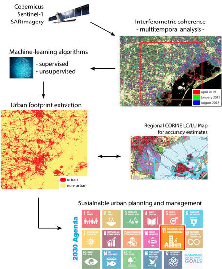
In order to guarantee the reusability of our approach on larger spatial and time scales, we adopted Open Data policies that involve the use of non-commercial satellite data. More specifically, we used imagery data provided by the Copernicus satellites, and in particular focusing on Sentinel-1 SAR (synthetic-aperture radar) imagery. This satellite system provides free data with global coverage at a weekly revisit time [38,39,40].
Unlike optical sensors, SAR systems can provide imagery data without being affected by cloud-cover, seasonality, and daytime variations, and can identify urban structures, as well. In fact, vertical structures such as buildings and other anthropic constructions act as corner reflectors, generating a particularly strong radar-echo signal (backscattered) that allows their easy identification. The sole exceptions are very large roads, central squares, and wide runways (larger than 40–50 m, considering we adopted an average Sentinel-1 geometric resolution of 15 m—see Section 2.3), which are likely to act as mirror-like reflectors. Due to the low frequency of such wide infrastructures in our study area and considering the scale of our analysis (see Section 2), we included them within the urban environment. On the contrary, smooth surfaces such as water bodies and rough irregular surfaces such as vegetated areas, respectively, act as mirror-like and diffuse reflectors, resulting in null or low backscattered intensity [41].
Therefore, due to their “double-bounce” effect, urban structures appear brighter in SAR images than all other surface types [13,41]. Moreover, the information provided by interferometric coherence allows better identification of urban areas, significantly reducing the number of outliers and anomalous values, with respect to the single backscattered images. Indeed, urban structures usually display high coherence due to their regular geometric properties and relatively constant physical parameters over time.
We focus on the analysis of an automatic and semi-automatic process to provide the extraction of urban features over non-urban areas, taking into account the use of machine-learning algorithms. In this work, we refer to “urban footprint” as the percentage of pixels classified as “urban” over the total number of pixels on a specified study area. In order to perform reliable accuracy assessments, we compared such results—obtained using 2018–2019 Sentinel data—with the land cover map of the Veneto Region, produced in 2015, as the most detailed and updated source of information for urban environment in our study area.
Accordingly, our goal is to test a methodology for local governments and public administrations that provides accurate and constantly updated information of urban footprint all over the Veneto Region, which is essential for strategic urban planning, resource management, and decision-making processes. This methodology may be a useful tool to support the production of geographic indicators able to address the targets of Goal 11 in the 2030 Agenda [6,7], by feeding and updating the Sustainable Development (SD) indicators associated with such targets [5,6,7]. In particular, this research intends to prepare a data workflow to help feed the SD indicators 11.3.1 “Ratio of land consumption rate to population growth rate” and 11.7.1 “Average share of the built-up area of cities that is open space for public use for all, by sex, age and persons with disabilities”. These indicators are included in targets 11.3 and 11.7, which aim, in a more general context, at enhancing sustainable urbanization through sustainable urban planning and management, and providing universal access to safe, inclusive, and accessible, green and public spaces [2].
Furthermore, local authorities and public administration constantly update and feed indicators for strategic land-monitoring and sustainable urban development [5,6,7], at both regional and national scales. In the case of Veneto Region in Italy, the constant update of such information is useful to feed not only regional SD indicators [42], but also the national statistical set [43,44], and the European monitoring framework.

2. Materials and Methods

2.1. RUS Copernicus: A New Frontier for Satellite Imagery Analysis

The ever-increasing availability of satellite imagery along with its growing complexity generates the need of a powerful computational environment able to analyze these data. In this regard, a consortium led by CS Group (Communication and Systèmes) developed the Research and User Support (RUS) Service, in response to a call made in 2016 by the European Commission [45]. It aims at developing an online free-access platform to promote the uptake of Copernicus data and support its applications. This service is available upon registration and under request to all citizens within the European Union (both public and private sector organizations and entities) [46].
During the development of this work, we requested and obtained five Level-A Virtual Machines with powerful computing environment (four CPU cores and 16 Gb RAM each), a set of open-source GIS software (such as ESA’s SNAP and QGIS), and shared cloud memory, allowing simultaneous processing and analysis of the same type of data. These VMs were fundamental to effectively run all the processes used in this work.

2.2. Sentinel-1 SAR Imagery

Sentinel-1 mission consists of two polar-orbiting satellites, carrying a single C-band synthetic-aperture radar (SAR) instrument operating in four exclusive acquisition modes, with different resolution (down to 5 m) and coverage (up to 400 km) [38,39,40].
In particular, in this work we made use of the Interferometric Wide swath (IW) mode products at Level-1 Single Look Complex (SLC). The IW swath mode acquires data with a 250 km swath at 5 × 20 m spatial resolution (for SLC products). The wide-swath coverage is achieved by employing the Terrain Observation by Progressive Scans (TOPS) acquisition mode, which acquires images by recording different subsets of echoes of the SAR aperture, which are called “bursts” [47]. Sentinel-1 IW SLC products contain a total of three (single polarization) or six (dual polarization) sub-swath images. For example, the images we examined consist of three sub-swaths (named IW1, IW2, and IW3), each including both polarization (VV and VH). Furthermore, each sub-swath image consists of a series of bursts.
Within this work, we perform multi-temporal analysis, collecting a series of images from July 2018 to April 2019 that are displayed in Table 1. In particular, in order to achieve interferometry with exact repeated coverage, we took into account only images derived from the same satellite sensor (Sentinel-1A), therefore within a bi-weekly revisit time.
Due to the low rate of urbanization in recent years in Italy (in terms of increase of built-up structures), the changes in urban footprint observed within the last couple of years can be neglected if considering the spatial resolution of the Sentinel-1 SAR sensors. Therefore, we can consider urban footprint as a constant value for all the Sentinel-1 images acquired within a single-year time frame.
All Sentinel mission data we used are available at the ESA Copernicus Open Access Hub [48].

2.3. Preprocessing Interferometric Coherence

The use and interpretation of SAR imagery require a series of complex pre-processing procedures, which we ran on ESA’s SNAP software within the RUS environment. Such procedures refer to standard preprocessing commonly applied to Sentinel-1 products to derive interferometric coherence [49]. In particular, we followed the approach described by RUS guidelines available in [50,51], which we summarize in Figure 1.
On all SAR input images we took into account both polarizations (VH and VV), so that the output coherence image is composed by two different raster files, related indeed to the different polarizations. As for the processing workflow, we identified one of the three sub-swaths from the original product, subsequently selecting only those bursts that cover our study areas. Furthermore, we computed the coherence estimation setting the range window size to the default value of 20 pixels. Lastly, for the terrain correction we used the Range-Doppler terrain correction, which involves the use of a digital elevation mode (DTM) automatically downloaded from the Sentinel-1 repository, choosing WGS84-UTM 32N as projected coordinate system and selecting an average output resolution of ≈15 m.
An example of output interferometric coherence image is displayed in Figure 2.

2.4. Supervised and Unsupervised Classification Applied to Interferometric Coherence

The output coherence image consists of two different bands, reporting interferometric coherence values (from 0 to 1) for two polarizations (VH and VV). Within this type of raster, it is possible to extract urban footprint by applying supervised (and unsupervised) classification algorithms.
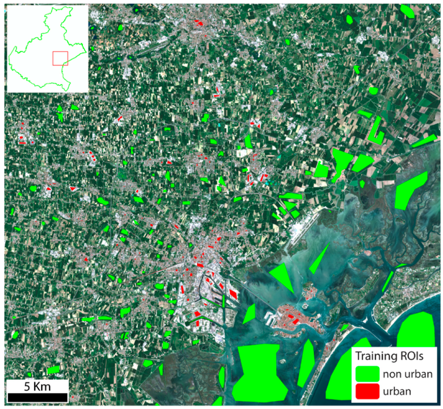
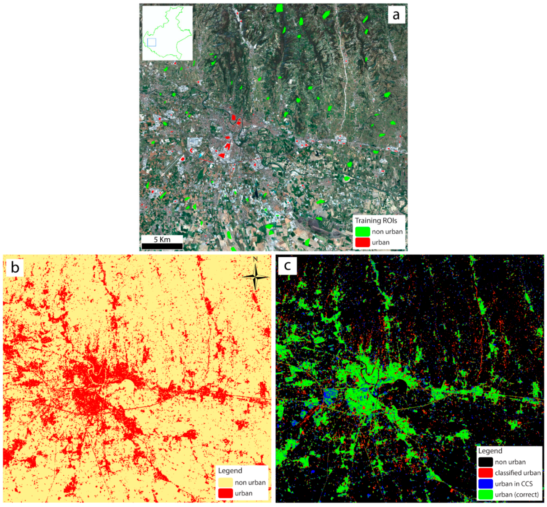
In the case of supervised classification, for training inputs we digitized the ROIs (regions of interest) over a Sentinel-2 image (Table 1) covering the same target area (Figure 3). Since we were interested in distinguishing only two different classes, i.e., urban and non-urban areas, when digitizing the ROIs, we aggregated all non-urban land cover types into the same class (such as sparse vegetation, forest, bare soil, and cultivated soil) (Figure 3). For further statistical analysis and high-resolution image validation of ROIs, the reader is referred to Table S1 and Figure S1, respectively, within the supplementary material. We then used such ROIs as input training sites for the classification algorithms applied to the SAR images. The Sentinel-2 images we used for this purpose are listed in Table 2. These Sentinel-2 images were processed in SNAP by extracting the bands on the visible wavelength range (bands 2, 3, and 4) and exporting the selected spatial subset into a GeoTIFF.
As for the supervised classification algorithms, we made use of the maximum likelihood (ML) [52] and the random forest (RF) classifiers [53,54], both available in SNAP. Specifically, the ML classifier in SNAP does not require setting of a threshold value for classifying pixels, thus no pixel will remain unclassified. On the other hand, for the RF classifier we specified the maximum number of decision trees, which we set to 500 as best value in order to obtain a good noise removal and a homogenous response [55]. We firstly applied supervised classification algorithms to a single coherence image (Figure 2), made by two distinct raster files, which indeed are related to the different polarizations of the same SAR image (VH and VV). Subsequently, we considered the use of multiple coherence images, taken within a longer period of time (see next section).
Ultimately, we also made use of unsupervised classification algorithms, in particular the K-means clustering, which does not require the digitalization of ROIs, but only the number of classes (or “clusters”) set for the classification map. In fact, the distinct backscattered intensity and interferometric coherence values of urban environments allow their sharp distinction from all other land cover types, regardless of the level of anthropization, weather conditions, or environmental parameters. For this reason, by setting only two classes for the K-means algorithm, it is likely that those classes will be automatically attributed to urban and non-urban pixels. We performed the unsupervised classification using the K-means algorithm available in SNAP. As in the case of the ML classifier, no threshold value is required for the K-means algorithm in SNAP, and we left the default value of 30 as number of iterations (which we found was a value high enough to identify the two cluster centers and successfully separate the two classes).

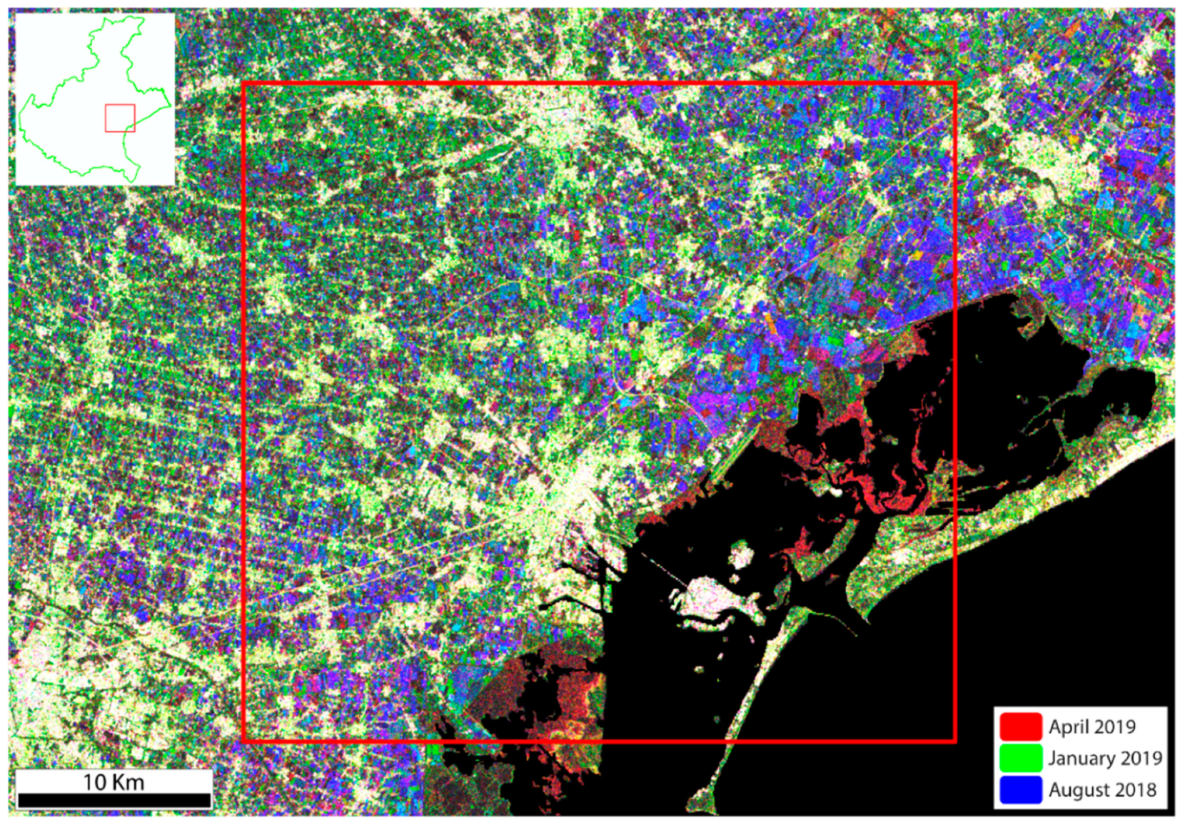
2.5. Multitemporal Analysis of Interferometric Coherence

Following the guidelines available in the RUS web material [50,51], we repeated the processing workflow of interferometric coherence, described in the previous section, to a series of Sentinel-1 images taken from April 2019 to July 2018 (Table 1), always related to the province of Venice and its surroundings. Subsequently, we produced a series of interferometric coherence images, every time processing two IW SLC images (taking into account both polarizations—VH and VV). Then, we stacked all coherence images into a single raster file using the Stack tool in SNAP. A sample result is displayed in Figure 4. By doing so, urban areas are likely to be identified more rigorously, progressively reducing the error and noise in the images and increasing the overall accuracy.
Lastly, we applied the same classification algorithms described in the previous section.

2.6. Testing Multitemporal Coherence on Other Test Areas

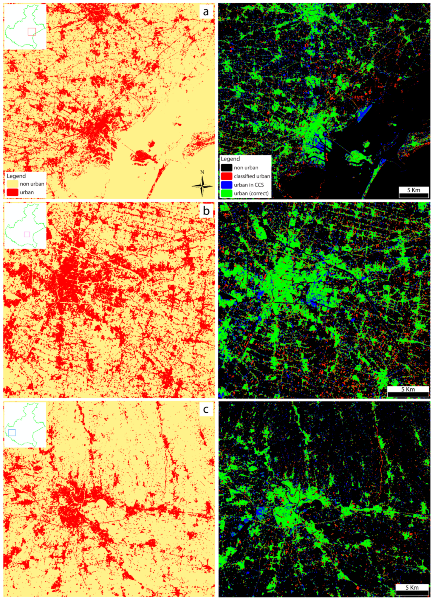
After testing this approach on the first study area (i.e., the Venice area), in order to verify the consistency and reliability of the method, we extended the same analysis on other test areas.
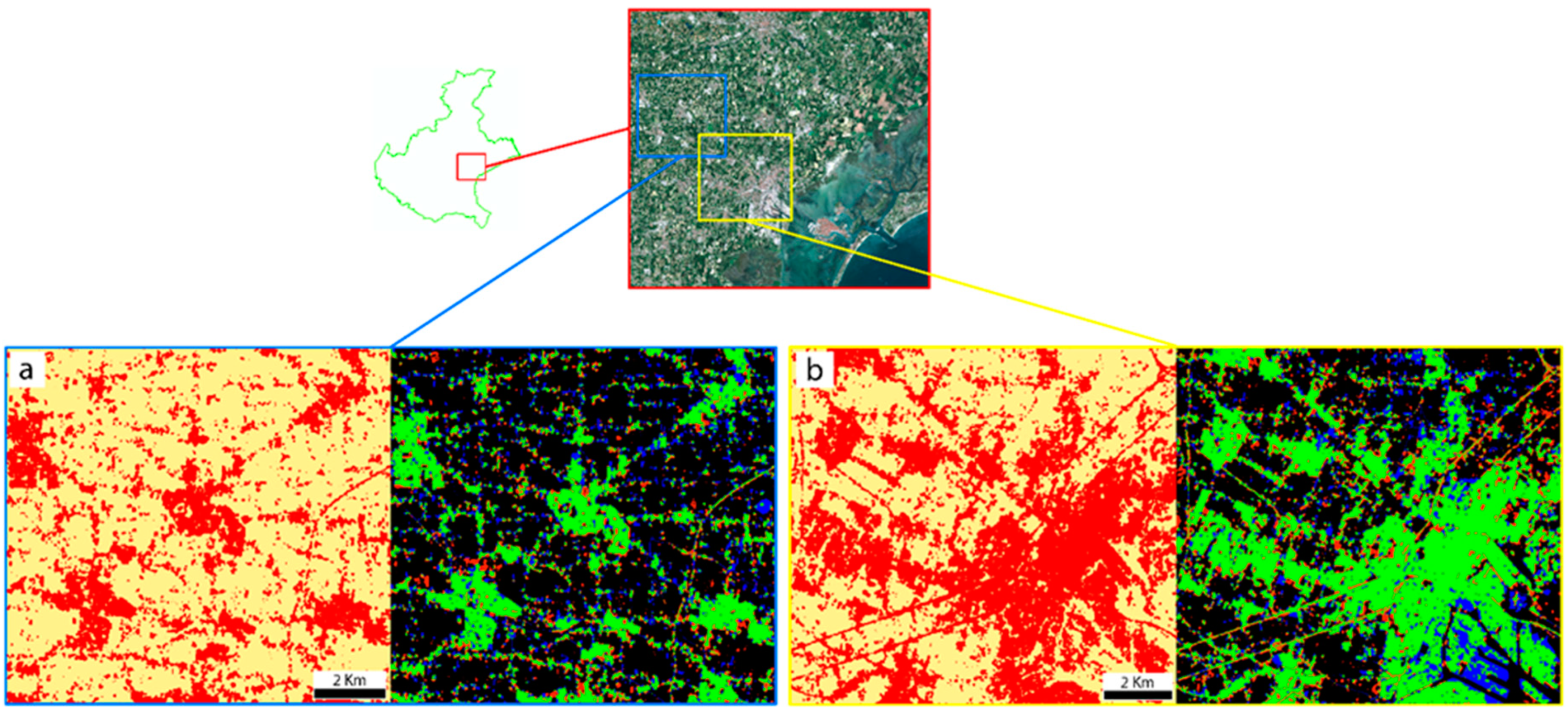
Firstly, we made use of the same ROIs digitized for the Venice region, but restricting the target area on which we applied the supervised classification algorithms. In this case, we tested the efficiency of our approach to extract urban footprint on smaller areas (at local scales), and over highly anthropized regions (see Section 3.3). We then repeated the same procedures on a large urbanized area around the city of Padua. Lastly, we tested the approach on a different environment, considering areas of similar size, taking into account the heterogeneous province of Verona, in the western boundary of the Veneto region, where dense residential and industrial areas alternate with sparsely populated (and thus less urbanized) mountain environments. We followed the same approach that involves the digitalization of ROIs over a Sentinel-2 image (Figure 3), which we used as input training sites for the supervised classification algorithms applied to the multitemporal set of interferometric coherence images.
We also applied unsupervised classification to these other test areas.

2.7. Land Use/Land Cover Map of the Veneto Region as Reference for Accuracy Assessments

When dealing with automatic processes that involve feature extraction and image classification, in order to estimate the reliability of any adopted approach, an accuracy assessment is always required. Within the Veneto Region, in particular, different sources related to urban environments were available, such as the land cover Map, the geo-topographic database, and cadastral data from the Land Registry (the Italian “Catasto”). These sources provide detailed multi-layer cartographic information of urban features and urban areas, with geometric resolution up to centimeters. However, we took into consideration only the land cover map of the Veneto Region (which we will refer to as “Carta di Copertura del Suolo”—CCS). Produced by Corvallis S.p.A. in 2015 through photointerpretation and ground truth information, as an update of previous versions, this map is the most reliable and up to date data source for the analysis of urban environment and the extraction of urban footprint. The map is available online as shapefile [55], i.e., as a vector file, with land cover codes included in the attribute table. These codes refer to the CORINE land cover classification (e.g., [56,57,58]). For further details on the CORINE land cover nomenclature, the reader is referred to Table S2 and Figure S2 in the supplementary material.
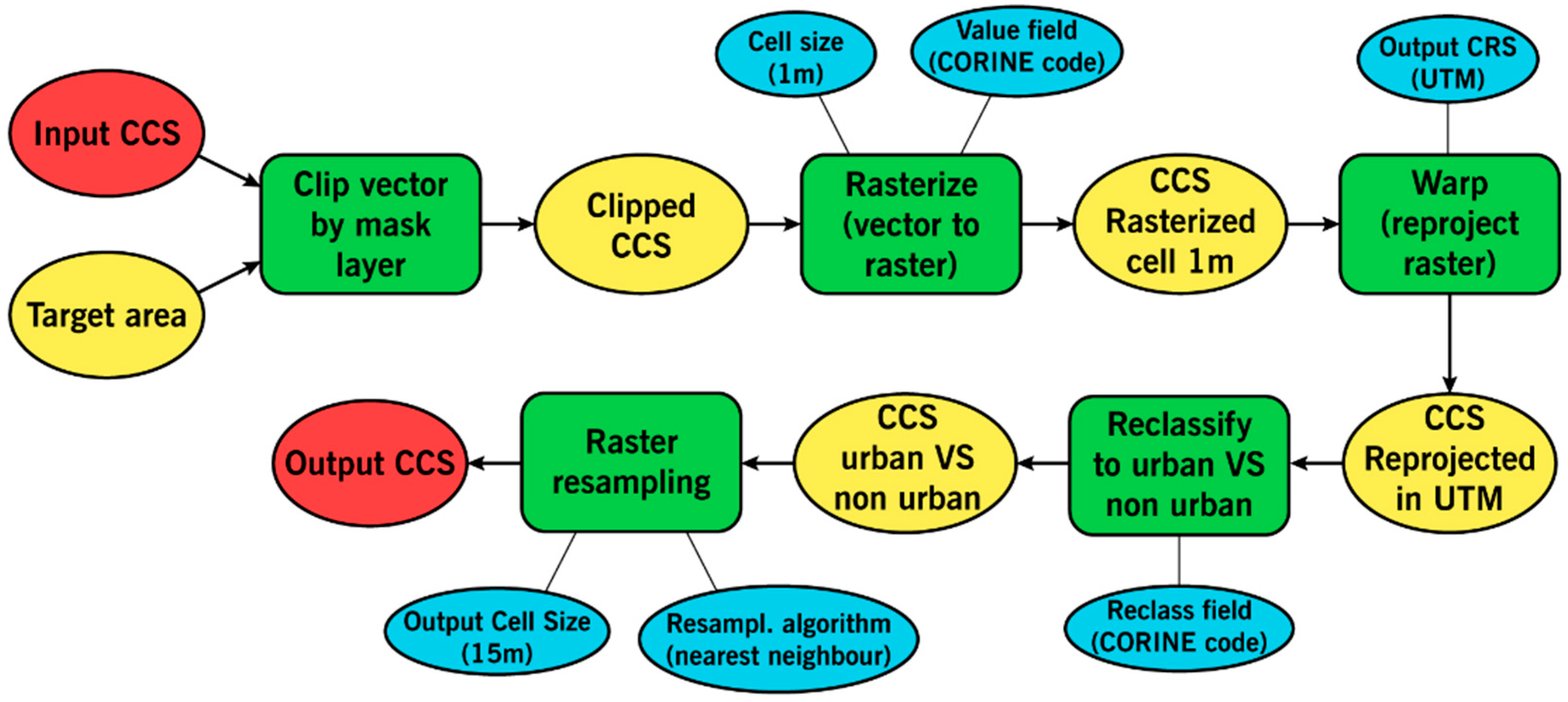
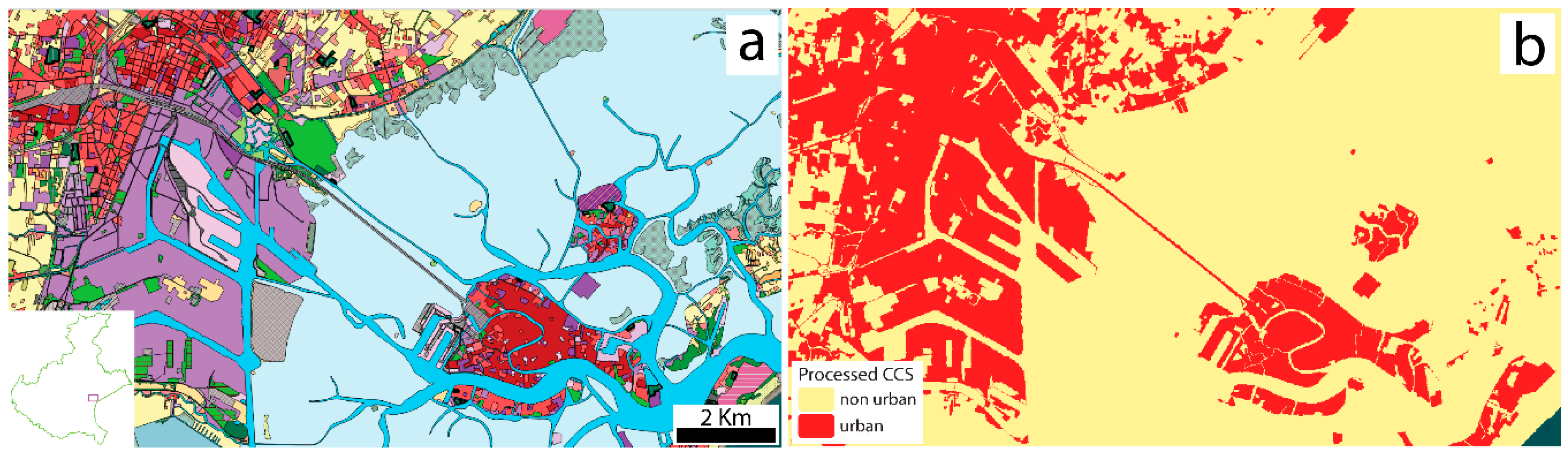
In order to perform accuracy assessments, we processed the vector input file of the CCS into a new raster file, with the same pixel characteristics of the classification images (i.e., urban footprint) obtained from Sentinel-1 SAR imagery. The processing workflow is summarized in Figure 5, whereas an example of the input and output map is displayed in Figure 6.
Once clipped into the study area, we converted the vector CCS into a raster image, attributing to the pixel values the codes of CORINE land cover classification. During the rasterization process, we set the initial pixel size of 1 m in order to avoid incorrect aggregation of different classes and preserve the high nominal resolution of the vector input file. Furthermore, we re-projected the CCS, originally projected in the Italian “Fuso 12” coordinate system (EPSG code 6876), into WGS84-UTM Zone 32N (EPSG 32632) as the Sentinel images.
The classification images produced from Sentinel-1 imagery consist of discrete rasters, with all pixels classified into either “urban” or “non-urban” values (with values 1 and 0, respectively). Therefore, once rasterized, we reclassified the CCS into “urban” and “non-urban” pixels, following the CORINE classification codes. In particular, we set as “urban” only the pixels included in Classes 1.1 and 1.2, referred to artificial surfaces, such as urban fabric and industrial, commercial, and transport units. On the other hand, we excluded Classes 1.3 and 1.4, respectively, “Mine, dump, construction sites” and “Artificial, non-agricultural vegetated areas”, since they are likely to be identified as non-urban surfaces on SAR images. We classified all other Classes 2, 3, and 4 (agricultural areas, forest and seminatural areas, and wetlands, respectively) as “non-urban”. Lastly, in order to perform the accuracy assessments, we resampled the output raster to the output Sentinel-1 image resolution, which is 15 m. The entire conversion process was run in QGIS. An example of a processed test area of the CCS is displayed in Figure 6b. Finally, once the CCS was properly pre-processed to match all the characteristics of the Sentinel-1 classification images, accuracy assessments were performed by means of the Semiautomatic Classification Plugin (SCP) implemented in QGIS. This plugin produces an error matrix indicating all statistical parameters, such as overall accuracy, user and producer accuracy, and Kappa hat coefficient (or Cohen’s kappa coefficient) (e.g., see [41]).

3. Results and Discussions

3.1. Supervised Classification Applied to Interferometric Coherence

We tested the ML classifier within a restricted area in the province of Venice, submitting the classified raster representing urban footprint (Figure 7a) to the SCP plugin for accuracy estimates, using the CCS as reference map (see Section 2.6). The results displayed in Figure 7b and Table 3 show an overall accuracy of ≈81% and a kappa hat classification value of ≈52%. In addition, when computing the percentage of urban footprint over non-urban areas, we obtained a value of ≈28% from the coherence image, which differs from the value computed within the CCS (≈26%) by less than 2% in the same area (Table 3).
By observing the accuracy image produced by the SCP plugin in QGIS (Figure 7b and Table 3), the value of ≈28% obtained from the ML classification includes the result of a balancing between a similar number of false positives and false negatives, respectively, in red and blue in Figure 7b. However, two large blue spots are visible in the central and east portion of the target area. These spots are related to local airport runways and flat port and industrial areas (mostly included within CORINE Classes 1.2.3 and 1.2.4—see Table S2 in the supplementary material for details). As stated in Section 1, anthropic flat areas that are significantly larger than SAR product geometric resolution (in this case larger than 15 m) may sometimes not be recognized as urban pixels, since they act as mirror-like reflectors. Nonetheless, considering the overall result, the misclassified pixels seem to be homogenously distributed over the target area. Such errors are likely to be attributed mainly to difference in resolutions between the original CCS and the Sentinel-1 products. In fact, considering the high geometric resolution of the input reference raster (higher than 1 m for the input shapefile), it is likely that during the preprocessing workflow of the CCS many pixels were aggregated (or “dissolved”) due to rasterization and resampling. Therefore, many small areas could have resulted in misclassified pixels. As a result, some background noise between the CCS and the Sentinel-1 products is inevitable but can be neglected from urban footprint estimates, since it uniformly affects both urban and non-urban pixels.

3.2. Stacking Multitemporal Image Series

Starting from the optimal results of urban footprint extraction obtained from a single coherence image, we expanded the same approach over a multitemporal series of images, acquired from July 2018 to April 2019 (see Section 2.4). Once the coherence stack is created (Figure 4), we ran the same classification workflow previously applied (with the same ROIs), firstly choosing random forest (RF) as classification algorithm (it requires less computational power than the ML classifier) (Figure 8a).
Results from accuracy assessments (Figure 8b and Table 4) display equally reliable values with respect to the single-coherence image. However, these results show a significant increase in accuracy, in particular with reduction of background noise (i.e., false positives and false negatives—see previous section). In fact, with an overall accuracy of ≈87% and a Kappa hat classification value of ≈65%, the urban footprint extracted from the coherence stack image differs from the value of the CCS again by less than 2%.
We repeated the same classification, using the ML classifier, and obtained even better results (Figure 9 and Table 5), with overall accuracy of ≈88%, Kappa hat coefficient of ≈66% and the percentage of urban footprint differing from that of the CCS by less than 1%.

3.3. Expanding Multitemporal Analysis to Other Test Areas

We tested the consistency of the method within smaller areas (local boundaries), performing additional supervised classifications (using ML classifier) and accuracy assessments over two restricted areas, clipped from the previous target area of the Venice region. The results displayed in Figure 10 provide additional constraints to the method, attesting high accuracy values at local scales (Table 6), with overall accuracy >80%, kappa coefficient >60%, and a percentage of urban footprint differing from that of the CCS by less than 2%, especially within highly anthropized areas (Figure 10b).
Subsequently, we took into account the same stack of coherence images and the same ROIs used in the previous attempts to produce an image of urban footprint in the highly anthropized region of the city of Padova and its surroundings (again, using the ML classifier) (Figure 11a). Accuracy assessments (Figure 11b and Table 7) display always the same values, and the same low error with respect of the CCS in terms of percentage of urban footprint (differing by less than 3%).
Lastly, we analyzed a different area in the province of Verona, which is composed by different environments (including mountain environment) and surface types. We repeated the processing workflow in SNAP on different sub-swaths of the same Sentinel-1 input images (Table 2). We digitized new ROIs (Figure 12a), always subdivided into “urban” and “non-urban” classes, performing the classification with the ML algorithm. Further statistical analysis and high-resolution image validation of ROIs are available in Table S1 and Figure S1, respectively, within the supplementary material.
Results from accuracy assessments (Figure 12c and Table 8) display the same high accuracy values previously obtained in other test areas, with overall accuracy close to ≈90%, kappa coefficient >60%, and a percentage error from the CCS lower than ≈1% in terms of urban footprint.

3.4. Unsupervised Classification: The Ultimate and Completely Automatic Approach to for Urban Mapping

Due to the successful results of multitemporal analysis of interferometric coherence combined with machine learning algorithms (using supervised classification algorithms, so far) we attempted a new approach to extract urban footprint, which involves the use of unsupervised image classification. In particular, once the stack of coherence images is obtained following the same processing workflow (Figure 1), we made use of the K-means classifier. Therefore, we performed unsupervised classification, applying the K-means algorithm to the same test areas previously analyzed with supervised classifications (Figure 13a–c, respectively, in the area of Venice, Padova, and Verona).
The results (Table 9a–c) are surprisingly similar to those obtained with the ML classifier, in some cases showing even higher accuracy, with overall accuracy >90% and kappa coefficient up to ≈70% (in the test area of Verona). The resulting urban footprint resulted again in percentage errors lower than 1% compared to the CCS.
These values confirm the reliability and accuracy of a completely automatic approach in terms of processing workflow, which, starting from a series of Sentinel-1 images, allows the extraction of urban footprint by means of multitemporal analysis of interferometric coherence and the use of unsupervised classification algorithms.

4. Conclusions

In this work, we aimed at developing an automatic (or semi-automatic) process able to map and monitor urban environment, and in particular to extract the spatial extent of urban features over non-urban areas (i.e., urban footprint). During the entire project development we had access to a series of Virtual Machines as powerful computational environment provided by the Copernicus RUS service [45,46].
When dealing with urban mapping, different data sources can be exploited in several different ways. In this work, we investigated the use of Sentinel-1 SAR imagery and in particular IW Level-1 SLC products. The high backscattered intensity of urban areas, acting as corner reflectors, proved to be highly effective when mapping urban environments. In particular, interferometric coherence highlights all surfaces with constantly high backscattered intensity, fixed shape, and constant physical parameters through time. Such surfaces are indeed urban areas.
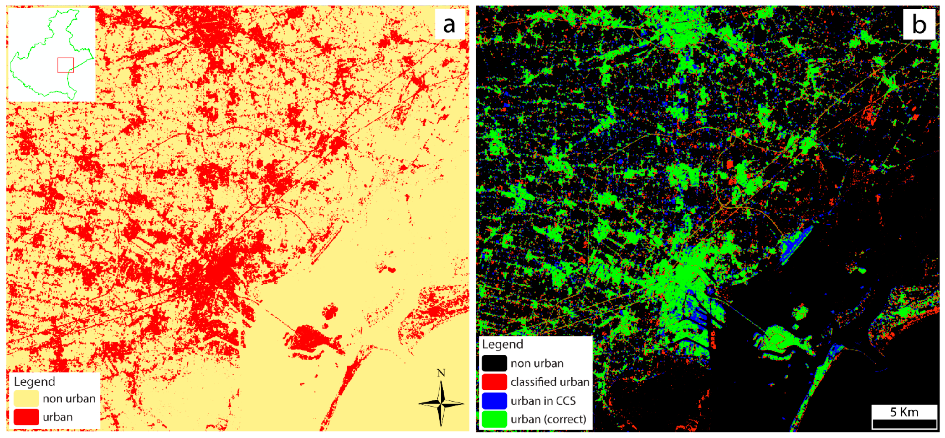
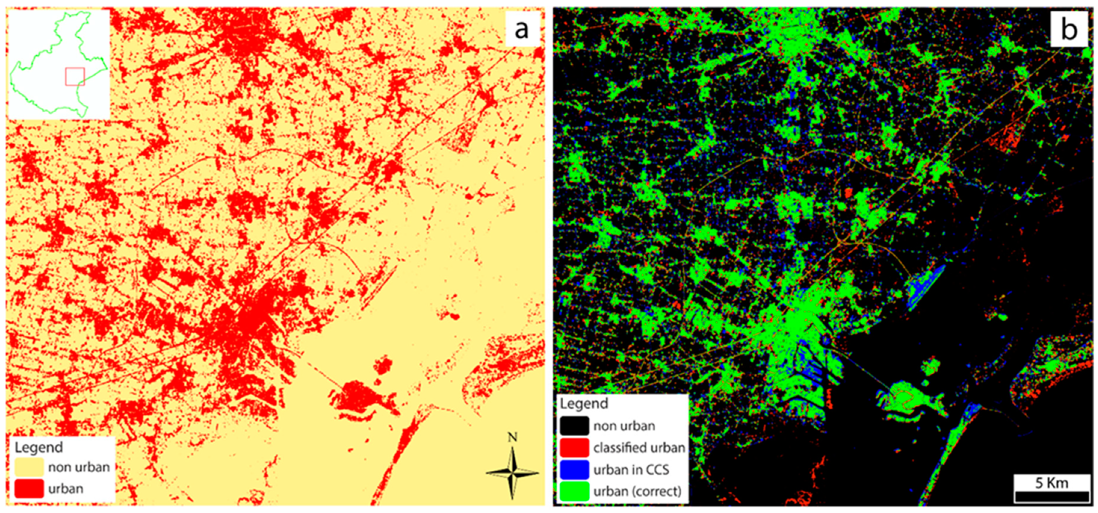
We stacked a series of coherence image related to a multitemporal series of images (from April 2019 to July 2018) in order to increase the accuracy of the classified coherence images. We performed a supervised classification using the random forest and maximum likelihood classifiers and then performed accuracy assessments, considering the properly preprocessed CCS as a reference. The classified images resulted in a high overall accuracy (up to 90%). Moreover, we obtained a percentage of urban footprint significantly precise compared to the values extracted from the CCS, with errors lower than 1%–2%. We repeated the same procedure on many other test areas, analyzing restricted areas around Venice, and other large areas around Padova and Verona (the latter including mountain environments, as well) obtaining similar accuracy values. Finally, we attempted a completely automatic approach in terms of processing workflow, which involves the use of unsupervised classification (with no need of digitization of training sites). We applied the K-means algorithm to the interferometric coherence stack image, exploiting the separability of urban environments with respect to all other surface types. Surprisingly, we obtained the same high accuracy values and, in some cases, even better results compared to the supervised classification approach.
By repeating these procedures within constant time intervals, it is possible to monitor the development of urban environment through time potentially in any region of the world. Considering our results, this methodology should provide reliable accuracy values within time intervals of 6–12 months. Moreover, since our methodology relies on open source tools and software, and globally available free data, we especially encourage the use of similar approaches for developing countries with emerging economies, considering more dynamic urban areas, as well.
As such, in the context of the 2030 Agenda for the Sustainable Development [2,3,4], in particular for Goal 11—Sustainable City and Communities, satellite imagery and Earth Observation technologies can play an important role for extracting and updating data to feed SD indicators. More specifically, we refer to targets 11.3 and 11.7, and in particular SD indicators 11.3.1 and 11.7.1 [5,6,7] (see Section 1 for details). Therefore, from the perspective of local governments and public authorities, we propose an organized dataflow coming from Sentinel-1 SAR data, in order to provide not only a helpful tool for a sustainable city development and urban planning at local and regional scales, but also help feeding such indicators for the national statistical set [43,44] and the European monitoring framework.
That being said, some limitations concerning Sentinel data still remain, mostly related to the limited geometric resolution of the Sentinel satellites with respect to other commercial satellites. Moreover, the first Copernicus Sentinel mission (Sentinel-1A) was launched in 2014, limiting so far the possibility of performing multitemporal analysis in the previous decades (using Sentinel data only). Nonetheless, the ever-increasing availability of high-resolution optical and radar satellite sensor, along with the growing awareness of open data policies, will definitely encourage the use of satellite images to tackle environmental changes and will promote new applications and technologies, in all fields, including urban applications.

Supplementary Materials

The following are available online at https://www.mdpi.com/2220-9964/9/6/375/s1, Table S1: Statistical analysis of ROIs areal extent, Figure S1: ROIs validation with high-resolution satellite imageries, Table S2: CORINE land cover nomenclature, Figure S2: CORINE land cover legend related to Figure 6a.

Author Contributions

Conceptualization, Andrea Semenzato, Umberto Trivelloni and Silvano De Zorzi; Data curation, Andrea Semenzato; Formal analysis, Andrea Semenzato; Investigation, Andrea Semenzato; Methodology, Andrea Semenzato; Project administration, Salvatore Eugenio Pappalardo, Daniele Codato, Umberto Trivelloni, Silvano De Zorzi and Massimo De Marchi; Resources, Umberto Trivelloni, Silvano De Zorzi and Massimo De Marchi; Software, Andrea Semenzato; Supervision, Salvatore Eugenio Pappalardo, Daniele Codato, Umberto Trivelloni, Silvano De Zorzi and Massimo De Marchi; Visualization, Andrea Semenzato; Writing—original draft, Andrea Semenzato; Writing—review and editing, Salvatore Eugenio Pappalardo, Daniele Codato, Sabrina Ferrari, Massimo De Marchi and Matteo Massironi. All authors have read and agreed to the published version of the manuscript.

Funding

This research received no external funding.

Acknowledgments

We particularly acknowledge the Regione del Veneto—U.O. Pianificazione Territoriale as well as the Professional Master in GIScience for project supervision and resource management. We also acknowledge the Research and User Support (RUS) Service for technical support with Virtual Machine operations and GIS software availability during the development of our work.

Conflicts of Interest

The authors declare no conflict of interest.

References

  1. Lambin, E.F.; Geist, H.J. Global land-use and land-cover change: What have we learned so far? Glob. Chang. News 2001, 46, 27–30. [Google Scholar]
  2. UN SDGs. Transforming Our World: The 2030 Agenda for Sustainable Development. Resolution Adopted by the UN General Assembly. 25 September 2015. Available online: https://sustainabledevelopment.un.org/post2015/transformingourworld (accessed on 5 March 2019).
  3. Pfeffer, K.; Georgiadou, Y. Global Ambitions, Local Contexts: Alternative Ways of Knowing the World. ISPRS Int. J. Geo-Inf. 2019, 8, 516. [Google Scholar] [CrossRef] [Green Version]
  4. Eurostat. Sustainable Development in the European Union: Monitoring Report on Progress towards the SDGS in an EU Context, 2019 ed.; Publications Office of the European Union: Luxembourg, 2019. [Google Scholar]
  5. Melchiorri, M.; Pesaresi, M.; Florczyk, A.; Corbane, C.; Kemper, T. Principles and Applications of the Global Human Settlement Layer as Baseline for the Land Use Efficiency Indicator—SDG 11.3.1. ISPRS Int. J. Geo-Inf. 2019, 8, 96. [Google Scholar] [CrossRef] [Green Version]
  6. Koch, F.; Krellenberg, K. How to Contextualize SDG 11? Looking at Indicators for Sustainable Urban Development in Germany. ISPRS Int. J. Geo-Inf. 2018, 7, 464. [Google Scholar] [CrossRef] [Green Version]
  7. Kraak, M.; Ricker, B.; Engelhardt, Y. Challenges of Mapping Sustainable Development Goals Indicators Data. ISPRS Int. J. Geo-Inf. 2018, 7, 482. [Google Scholar] [CrossRef] [Green Version]
  8. European Global Navigation Satellite System and Copernicus: Supporting the Sustainable Development Goals. Building Blocks towards the 2030 Agenda; United Nations Office at Vienna: Vienna, Austria, 2018.
  9. Donnay, J.P.; Barnsley, M.J.; Longley, P.A. Remote Sensing and Urban Analysis; Taylor and Francis: London, UK, 2001. [Google Scholar]
  10. Herold, M.; Goldstein, N.C.; Clarke, K.C. The spatiotemporal form of urban growth: Measurement, analysis and modeling. Remote Sens. Environ. 2003, 86, 286–302. [Google Scholar] [CrossRef]
  11. Taubenböck, H.; Wegmann, M.; Berger, C.; Breunig, M.; Roth, A.; Mehl, H. Spatiotemporal analysis of Indian megacities. In Proceedings of the International Archives of the Photogrammetry, Remote Sensing and Spatial Information Sciences, Beijing, China, 3–11 July 2008; Volume 10, pp. 75–82. [Google Scholar]
  12. Xu, H. A new index for delineating built-up land features in satellite imagery. Int. J. Remote Sens. 2008, 29, 4269–4276. [Google Scholar] [CrossRef]
  13. Small, C.; Okujeni, A.; van der Linden, S.; Waske, B. Remote Sensing of Urban Environments. Compr. Remote Sens. 2018, 96–127. [Google Scholar] [CrossRef]
  14. Wu, C. Normalized spectral mixture analysis for monitoring urban composition using ETM+ imagery. Remote Sens. Environ. 2004, 93, 480–492. [Google Scholar] [CrossRef]
  15. Bhatta, B. Analysis of Urban Growth and Sprawl from Remote Sensing Data; Springer: Berlin/Heidelberg, Germany, 2010. [Google Scholar]
  16. Small, C. High spatial resolution spectral mixture analysis of urban reflectance. Remote Sens. Environ. 2003, 88, 170–186. [Google Scholar] [CrossRef]
  17. Bhatta, B. Analysis of urban growth pattern using remote sensing and GIS: A case study of Kolkata, India. Int. J. Remote Sens. 2009, 30, 4733–4746. [Google Scholar] [CrossRef]
  18. Powell, R.L.; Roberts, D.A.; Dennison, P.E.; Hess, L.L. Sub-pixel mapping of urban land cover using multiple endmember spectral mixture analysis: Manaus, Brazil. Remote Sens. Environ. 2007, 106, 253–267. [Google Scholar] [CrossRef]
  19. Guindon, B.; Zhang, Y.; Dillabaugh, C. Landsat urban mapping based on a combined spectral-spatial methodology. Remote Sens. Environ. 2004, 92, 218–232. [Google Scholar] [CrossRef]
  20. Khatami, R.; Mountrakis, G.; Stehman, S.V. A meta-analysis of remote sensing research on supervised pixel-based land-cover image classification processes: General guidelines for practitioners and future research. Remote Sens. Environ. 2016, 177, 89–100. [Google Scholar] [CrossRef] [Green Version]
  21. Dewan, A.M.; Yamaguchi, Y. Land use and land cover change in Greater Dhaka, Bangladesh: Using remote sensing to promote sustainable urbanization. Appl. Geogr. 2009, 29, 390–401. [Google Scholar] [CrossRef]
  22. He, C.; Shi, P.; Xie, D.; Zhao, Y. Improving the normalized difference built-up index to map urban built-up areas using a semiautomatic segmentation approach. Remote Sens. Lett. 2010, 1, 213–221. [Google Scholar] [CrossRef] [Green Version]
  23. Zha, Y.; Gao, J.; Ni, S. Use of normalized difference built-up index in automatically mapping urban areas from TM imagery. Int. J. Remote Sens. 2003, 24, 583–594. [Google Scholar] [CrossRef]
  24. Badlani, B.; Patel, A.N.; Patel, K.; Kalubarme, M.H. Urban Growth Monitoring using Remote Sensing and Geo-Informatics: Case Study of Gandhinagar, Gujarat State (India). Int. J. Geosci. 2017, 8, 563–576. [Google Scholar] [CrossRef] [Green Version]
  25. Bhatti, S.S.; Tripathi, N.K. Built-up area extraction using Landsat 8 OLI imagery. GISci. Remote Sens. 2014, 51, 445–467. [Google Scholar] [CrossRef] [Green Version]
  26. Valdiviezo-N, J.C.; Téllez-Quiñones, A.; Salazar-Garibay, A.; López-Caloca, A.A. Built-up index methods and their applications for urban extraction from Sentinel 2A satellite data: discussion. J. Opt. Soc. Am. A 2018, 35, 35. [Google Scholar] [CrossRef]
  27. Gamba, P.; Aldrighi, M.; Stasolla, M. Robust Extraction of Urban Area Extents in HR and VHR SAR Images. IEEE J. Sel. Top. Appl. Earth Obs. Remote Sens. 2011, 4, 27–34. [Google Scholar] [CrossRef]
  28. Gamba, P.; Lisini, G. Fast and Efficient Urban Extent Extraction Using ASAR Wide Swath Mode Data. IEEE J. Sel. Top. Appl. Earth Obs. Remote Sens. 2013, 6, 2184–2195. [Google Scholar] [CrossRef]
  29. Du, P.; Samat, A.; Waske, B.; Liu, S.; Li, Z. Random Forest and Rotation Forest for fully polarized SAR image classification using polarimetric and spatial features. ISPRS J. Photogramm. Remote Sens. 2015, 105, 38–53. [Google Scholar] [CrossRef]
  30. Grey, W.; Luckman, A.J. Mapping urban extent using satellite radar interferometry. Photogramm. Eng. Remote Sens. 2003, 69, 957–961. [Google Scholar] [CrossRef]
  31. Holobâcă, I.H.; Ivan, K.; Alexe, M. Extracting built-up areas from Sentinel-1 imagery using land-cover classification and texture analysis. Int. J. Remote Sens. 2019, 40, 8054–8069. [Google Scholar] [CrossRef]
  32. Cao, H.; Zhang, H.; Wang, C.; Zhang, B. Operational built-up areas extraction for cities in China using Sentinel-1 SAR data. Remote Sens. 2018, 10, 1–20. [Google Scholar] [CrossRef] [Green Version]
  33. Lehner, A.; Naeimi, V.; Steinnocher, K. Sentinel-1 for Urban Areas—Comparison between Automatically Derived Settlement Layers from Sentinel-1 Data and Copernicus High Resolution Information Layers. In Proceedings of the 3rd International Conference on Geographical Information Systems Theory, Applications and Management, Porto, Portugal, 27–28 April 2017; pp. 43–49. [Google Scholar] [CrossRef]
  34. Weng, Q. Thermal infrared remote sensing for urban climate and environmental studies: Methods, applications, and trends. ISPRS J. Photogramm. Remote Sens. 2009, 64, 335–344. [Google Scholar] [CrossRef]
  35. Zhan, W.; Chen, Y.; Zhou, J.; Wang, J.; Liu, W.; Voogt, J.; Zhu, X.; Quan, J.; Li, J. Disaggregation of remotely sensed land surface temperature: Literature survey, taxonomy, issues, and caveats. Remote Sens. Environ. 2013, 131, 119–139. [Google Scholar] [CrossRef]
  36. Yu, B.; Shu, S.; Liu, H.; Song, W.; Wu, J.; Wang, L.; Chen, Z. Object-based spatial cluster analysis of urban landscape pattern using nighttime light satellite images: A case study of China. Int. J. Geogr. Inf. Sci. 2014, 28, 2328–2355. [Google Scholar] [CrossRef]
  37. Small, C. Comparative analysis of urban reflectance and surface temperature. Remote Sens. Environ. 2006, 104, 168–189. [Google Scholar] [CrossRef]
  38. Attema, E.; Snoeij, P.; Duesmann, B.; Davidson, M.; Floury, N.; Rosich, B.; Rommen, B.; Levrini, G. GMES Sentinel-1 mission and system. Eur. Space Agency (Spec. Publ.) 2009, 668, 26–30. [Google Scholar]
  39. Snoeij, P.; Attema, E.; Torres, R.; Levrini, G. C-SAR Instrument Design for the Sentinel-1 Mission. In Proceedings of the 2010 IEEE Radar Conference, Washington, DC, USA, 10–14 May 2010; pp. 25–30. [Google Scholar]
  40. Torres, R.; Snoeij, P.; Geudtner, D.; Bibby, D.; Davidson, M.; Attema, E.; Potin, P.; Rommen, B.; Floury, N.; Brown, M.; et al. GMES Sentinel-1 mission. Remote Sens. Environ. 2012, 120, 9–24. [Google Scholar] [CrossRef]
  41. Richards, J.A. Remote Sensing Digital Image Analysis, 5th ed.; Springer: Berlin/Heidelberg, Germany, 2013; pp. 1–25. [Google Scholar] [CrossRef]
  42. Veneto Region: Local and National Reports of Monitoring Indicators (2030 Agenda). Available online: https://venetosostenibile.regione.veneto.it/dati-territoriali (accessed on 15 May 2019).
  43. National Statistical Set (ISTAT—Italy)—List of National Monitoring Indicators Related to SDG 11. Available online: https://www.istat.it/storage/SDGs/SDG_11_Italy.pdf (accessed on 11 May 2019).
  44. ISTAT Indicators for the United Nations Sustainable Development Goals. Available online: https://www.istat.it/en/well-being-and-sustainability/sustainable-development-goals/istat-indicators-for-sustainable-development (accessed on 15 May 2019).
  45. Palazzo, F.; Šmejkalová, T.; Castro-Gomez, M.; Rémondière, S.; Scarda, B.; Bonneval, B.; Gilles, C.; Guzzonato, E.; Mora, B. RUS: A New Expert Service for Sentinel Users. Proceedings 2018, 2, 369. [Google Scholar] [CrossRef] [Green Version]
  46. Copernicus Research and User Support (RUS). Available online: https://rus-copernicus.eu/ (accessed on 3 March 2019).
  47. De Zan, F.; Guarnieri, A.M. TOPSAR: Terrain observation by progressive scans. IEEE Trans. Geosci. Remote Sens. 2006, 44, 2352–2360. [Google Scholar] [CrossRef]
  48. ESA Copernicus—Open Access Hub. Available online: https://scihub.copernicus.eu/ (accessed on 25 February 2019).
  49. Yague-Martinez, N.; Prats-Iraola, P.; Rodriguez Gonzalez, F.; Brcic, R.; Shau, R.; Geudtner, D.; Eineder, M.; Bamler, R. Interferometric Processing of Sentinel-1 TOPS Data. IEEE Trans. Geosci. Remote Sens. 2016, 54, 2220–2234. [Google Scholar] [CrossRef] [Green Version]
  50. RUS Web Material: Urban Classification with Sentinel-1. Available online: https://rus-training.eu/training/urban-classification-with-sentinel-1 (accessed on 13 March 2019).
  51. RUS Web Material: Urban Classification with Sentinel-1. Case Study: Germany. 2018. Available online: https://rus-copernicus.eu/portal/wp-content/uploads/library/education/training/LAND06_UrbanClassification_Germany.pdf (accessed on 13 March 2019).
  52. Aldrich, J.R.A. Fisher and the making of maximum likelihood 1912—1922. Stat. Sci. 1997, 12, 162–176. [Google Scholar] [CrossRef]
  53. Breiman, L. Random Forests. Mach. Learn. 2001, 45, 5–32. [Google Scholar] [CrossRef] [Green Version]
  54. Belgiu, M.; Drăgu, L. Random forest in remote sensing: A review of applications and future directions. ISPRS J. Photogramm. Remote Sens. 2016, 114, 24–31. [Google Scholar] [CrossRef]
  55. Liaw, A.; Wiener, M. Classification and Regression by randomForest. R News 2. R News 2002, 3, 18–22. [Google Scholar]
  56. Bossard, M.; Feranec, J.; Otahel, J. CORINE Land Cover Technical Guide—Addendum 2000; European Environment Agency: Copenhagen, Denmark, 2000. [Google Scholar]
  57. Büttner, G.; Feranec, J.; Jaffrain, G. Corine Land Cover Update 2000. Technical Guidelines; European Environment Agency: Copenhagen, Denmark, 2002; pp. 1–56. [Google Scholar]
  58. Büttner, G.; Feranec, J.; Jaffrain, G.; Mari, L.; Maucha, G.; Soukup, T. The CORINE land cover 2000 project. EARSeL eProc. 2004, 3, 331–346. [Google Scholar]
Figure 1. Preprocessing workflow used to produce Sentinel-1 interferometric coherence images in SNAP. The “Read” and “Read (2)” commands represent the two Sentinel-1 input files, while “Write” represents the output file.
Ijgi 09 00375 g001
Figure 2. Coherence image of the Venice area, within the Veneto Region, represented in the bottom left frame with its green border within the Italian border (in red the study area). We produced this image from two Sentinel-1A images acquired on 01 April 2019 and 20 March 2019 (VH polarization only). In this sample area, we selected sub-swath number 2 (IW2) and bursts 5–9. Urban areas appear distinctively brighter than all other land cover types, with coherence value generally greater than 0.7.
Ijgi 09 00375 g002
Figure 3. ROIs (regions of interest) digitized over a Sentinel-2A (MSI Level 2A) image acquired in July 2018.
Ijgi 09 00375 g003
Figure 4. Raster image related to a stack of interferometric coherence images, produced from Sentinel-1A images from July 2018 to April 2019. In particular, this image displays in a band composition three coherence images from April 2019, January 2019, and August 2018, respectively, in the red, green, and blue channel. Urban areas are recognizable by their distinctively brighter color compared to all other land cover types.
Ijgi 09 00375 g004
Figure 5. The complete processing workflow applied to the CCS (Carta di Copertura del Suolo) for accuracy assessments. We ran all the workflow within the QGIS environment, by means of GDAL and SAGA algorithms.
Ijgi 09 00375 g005
Figure 6. (a) Example in the Venice lagoon from the CCS (Carta di Copertura del Suolo) of the Veneto Region, updated to 2015. Legend colors refer to the CORINE land cover classification, which we do not report in this image for the sake of simplicity (see text for details). For additional details on the legend the reader is referred to Figure S2 in the supplementary material. (b) Same image of (a), preprocessed following the workflow displayed in Figure 5, displaying urban and non-urban pixels. We considered the same test area as in Figure 5. Pixel values are 1 and 0, respectively, for urban and non-urban pixels.
Ijgi 09 00375 g006
Figure 7. (a) Supervised classification (using maximum likelihood (ML) classifier) run over an interferometric coherence image including both polarizations (VH and VV), processed from two Sentinel-1A images acquired in February 2019. (b) Accuracy assessments using CCS as a reference map. This image displays the distribution of correctly classified and misclassified pixels. The black and green pixels are related to pixels correctly classified as “non-urban” and “urban”, respectively. In red are pixels erroneously classified as urban pixels (non-urban in the CCS)—false positives; whereas in blue are urban pixels in the CCS, but classified as “non-urban” in the ML classification—false negatives.
Ijgi 09 00375 g007
Figure 8. (a) Supervised classification (using random forest (RF) classifier) run over a stack of interferometric coherence images produced processing a time series of Sentinel-1A images acquired from April 2019 to July 2018. (b) Accuracy assessments using CCS as a reference map (see Figure 7 for details).
Ijgi 09 00375 g008
Figure 9. (a) Supervised classification (using ML classifier) run over a stack of interferometric coherence images produced processing a time series of Sentinel-1A images acquired from April 2019 to July 2018. (b) Accuracy assessments using CCS as a reference map.
Ijgi 09 00375 g009
Figure 10. Supervised ML classification (a) and related accuracy assessments (b) performed on two restricted areas included within the main study area taken into account so far, using a series of coherence images that were processed from Sentinel-1A images (April 2019–July 2018). For a better visualization, in this image we omitted the Legend (see Figure 7, Figure 8 and Figure 9).
Ijgi 09 00375 g010
Figure 11. (a) Supervised classification (using ML classifier) run over the same stack of interferometric coherence images used for the Venice area, but in a different target area, which includes the province of Padova. (b) Accuracy assessments using CCS as a reference map.
Ijgi 09 00375 g011
Figure 12. (a) The test area of Verona as seen from a Sentinel-2B image from March 2019 (see Table 2), displaying the ROIs digitized as training inputs for machine learning algorithms. (b) Supervised classification (using ML classifier) run over the series of interferometric coherence images previously considered. (c) Accuracy assessments using CCS as a reference map. The scale indicated in (a) is equivalent in all three images, therefore we did not replicate it for a better visibility of the result images.
Ijgi 09 00375 g012
Figure 13. K-means unsupervised classification and related accuracy assessments (using CCS as reference map) performed on the same test areas previously analyzed with supervised classification algorithms. (a) Venice study area. (b) Padova study area. (c) Verona study area. For all the study areas, the scale indicated in the accuracy image on the right is equivalent to the relative classification image on the left, therefore we did not replicate it for better visibility.
Ijgi 09 00375 g013
Table 1. All the Sentinel-1 images used in this work. Downloaded from the Sentinel Open Access Hub [48].
Sentinel-1 ImageAcquisition Date
S1A_IW_SLC_1SDV_20190425T051855_20190425T051922_026542_030810_5EE325 April 2019
S1A_IW_SLC_1SDV_20190401T051854_20190401T051921_026592_02FB56_3D0201 April 2019
S1A_IW_SLC_1SDV_20190320T051854_20190320T051921_026417_02F4DE_742820 March 2019
S1A_IW_SLC_1SDV_20190308T051854_20190308T051921_026242_02EE6B_907108 March 2019
S1A_IW_SLC_1SDV_20190224T051854_20190224T051920_026067_02E820_EDE724 February 2019
S1A_IW_SLC_1SDV_20190212T051854_20190212T051921_025892_02E1E6_044E12 February 2019
S1A_IW_SLC_1SDV_20190131T051854_20190131T051921_025717_02DBAB_B7C731 January 2019
S1A_IW_SLC_1SDV_20190107T051855_20190107T051922_025367_02CEF3_326707 January 2019
S1A_IW_SLC_1SDV_20181226T051855_20181226T051922_025192_02C8A1_68F526 December 2018
S1A_IW_SLC_1SDV_20181214T051855_20181214T051922_025017_02C24E_64ED14 December 2018
S1A_IW_SLC_1SDV_20181120T051857_20181120T051923_024667_02B608_37DF20 November 2018
S1A_IW_SLC_1SDV_20181108T051857_20181108T051924_024492_02AF94_AAE508 November 2018
S1A_IW_SLC_1SDV_20181027T051857_20181027T051924_024317_02A97B_468627 October 2018
S1A_IW_SLC_1SDV_20181015T051857_20181015T051924_024142_02A3DE_8F3515 October 2018
S1A_IW_SLC_1SDV_20180921T051856_20180921T051923_023792_02986D_908A21 September 2018
S1A_IW_SLC_1SDV_20180909T051856_20180909T051923_023617_0292CA_566509 September 2018
S1A_IW_SLC_1SDV_20180816T051855_20180816T051922_023267_028792_045C16 August 2018
S1A_IW_SLC_1SDV_20180804T051854_20180804T051921_023092_0281EF_C56B04 August 2018
S1A_IW_SLC_1SDV_20180723T051854_20180723T051920_022917_027C74_723A23 July 2018
S1A_IW_SLC_1SDV_20180711T051853_20180711T051920_022742_0276FD_1EC011 July 2018
Table 2. All the Sentinel-2 images used in this work. Downloaded from the Sentinel Open Access Hub [48].
Sentinel-2 ImageAcquisition Date
S2B_MSIL2A_20190330T101029_N0211_R022_T32TPR_20190330T14432830/03/2019
S2A_MSIL2A_20180718T101031_N0208_R022_T32TQR_20180718T18014618/07/2018
Table 3. Error matrix related to ML classification performed on the coherence image from February 2019. Urban footprint is computed as the percentage of urban pixels over the total number of pixels.
Reference Data (CCS) Urban Footprint
Classified Data (ML)Non-UrbanUrbanTotalReference Data (CCS)Classified Data (ML)
Non-urban1,621,709218,3331,840,04226.305428.2814
Urban269,028456,570725,598
Total1,890,737674,9032,565,640
Producer accuracy85.771367.6497
User accuracy88.134362.9233
Overall accuracy81.0043
Kappa hat classification0.5216
Table 4. Error matrix related to RF classification performed on the multitemporal coherence image in the Venice study area.
Reference Data (CCS) Urban Footprint
Classified Data (RF)Non-UrbanUrbanTotalReference Data (CCS)Classified Data (RF)
Non-urban3,999,913303,0394,302,95221.962923.3680
Urban381,934930,1961,312,130
Total4,381,8471,233,2355,615,082
Producer accuracy91.283775.4273
User accuracy92.957470.8921
Overall accuracy87.8012
Kappa hat classification0.6521
Table 5. Error matrix related to ML classification performed on the multitemporal coherence image in the Venice study area.
Reference Data (CCS) Urban Footprint
Classified Data (ML)Non-UrbanUrbanTotalReference Data (CCS)Classified Data (ML)
Non-urban4,031,904309,1494,341,05321.962922.6894
Urban349,943924,0861,274,029
Total4,381,8471,233,2355,615,082
Producer accuracy92.013874.9319
User accuracy92.878572.5326
Overall accuracy88.2621
Kappa hat classification0.6616
Table 6. Error matrix related to ML classification performed on the two restricted areas in the Venice region. Letters (a) and (b) are referred to the same letters in Figure 10.
(a)
Reference Data (CCS) Urban Footprint
Classified Data (ML)Non-UrbanUrbanTotalReference Data (CCS)Classified Data (ML)
Non-urban305,85539,855345,71029.044127.7966
Urban33,88299,208133,090
Total339,737139,063478,800
Producer accuracy90.027071.3403
User accuracy88.471674.5420
Overall accuracy84.5996
Kappa hat classification0.6216
(b)
Reference Data (CCS) Urban Footprint
Classified Data (ML)Non-UrbanUrbanTotalReference Data (CCS)Classified Data (ML)
Non-urban229,20246,794275,99647.629448.0527
Urban49,043206,261255,304
Total278,245253,055531,300
Producer accuracy82.374281.5084
User accuracy83.045480.7904
Overall accuracy81.9618
Kappa hat classification0.6386
Table 7. Error matrix related to ML classification performed on the target area of Padova (Figure 11).
Reference Data (CCS) Urban Footprint
Classified Data (ML)Non-UrbanUrbanTotalReference Data (CCS)Classified Data (ML)
Non-urban1,637,326184,9751,822,30133.107535.7755
Urban260,678754,4141,015,092
Total1,898,004939,3892,837,393
Producer accuracy86.265780.3090
User accuracy89.849474.3198
Overall accuracy84.2936
Kappa hat classification0.6525
Table 8. Error matrix related to ML classification performed on the target area of Verona (Figure 12).
Reference Data (CCS) Urban Footprint
Classified Data (ML)Non-UrbanUrbanTotalReference Data (CCS)Classified Data (ML)
Non-urban3,307,080229,6083,536,68818.924019.7720
Urban267,827604,815872,642
Total3,574,907834,4234,409,330
Producer accuracy92.508172.4830
User accuracy93.507869.3085
Overall accuracy88.7186
Kappa hat classification0.6387
Table 9. Error matrix related to K-means classification performed on the target area of Venice (a), Padova (b) and Verona (c) (see Figure 13).
(a)
Reference Data (CCS) Urban Footprint
Classified Data (K-means)Non-UrbanUrbanTotalReference Data (CCS)Classified Data (K-means)
Non-urban4,090,775371,4084,462,18321.965420.5671
Urban292,854862,5111,155,365
Total4,383,6291,233,9195,617,548
Producer accuracy93.319469.9001
User accuracy91.676574.6527
Overall accuracy88.1752
Kappa hat classification0.6470
(b)
Reference Data (CCS) Urban Footprint
Classified Data (K-means)Non-UrbanUrbanTotalReference Data (CCS)Classified Data (K-means)
Non-urban1,644,911221,6641,866,57533.104834.2606
Urban254,482718,298972,780
Total1,899,393939,9622,839,355
Producer accuracy86.601976.4178
User accuracy88.124673.8397
Overall accuracy83.2305
Kappa hat classification0.6247
(c)
Reference Data (CCS) Urban Footprint
Classified Data (K-means)Non-UrbanUrbanTotalReference Data (CCS)Classified Data (K-means)
Non-urban3,408,678238,5883,647,26618.924017.2391
Urban164,748595,298760,046
Total3,573,426833,8864,407,312
Producer accuracy95.389671.3884
User accuracy93.458478.3239
Overall accuracy90.8485
Kappa hat classification0.6912

