Article

Constructing Geospatial Concept Graphs from Tagged Images for Geo-Aware Fine-Grained Image Recognition

Graduate School of Engineering, Osaka University, Suita, Osaka 565-0871, Japan
*
Author to whom correspondence should be addressed.
ISPRS Int. J. Geo-Inf. 2020, 9(6), 354; https://doi.org/10.3390/ijgi9060354
Submission received: 27 April 2020 / Revised: 16 May 2020 / Accepted: 25 May 2020 / Published: 27 May 2020

Abstract

:
While visual appearances play a main role in recognizing the concepts captured in images, additional information can provide complementary information for fine-grained image recognition, where concepts with similar visual appearances such as species of birds need to be distinguished. Especially for recognizing geospatial concepts, which are observed only at specific places, geographical locations of the images can improve the recognition accuracy. However, such geo-aware fine-grained image recognition requires prior information about the visual and geospatial features of each concept or the training data composed of high-quality images for each concept associated with correct geographical locations. By using a large number of images photographed in various places and described with textual tags which can be collected from image sharing services such as Flickr, this paper proposes a method for constructing a geospatial concept graph which contains the necessary prior information for realizing the geo-aware fine-grained image recognition, such as a set of visually recognizable fine-grained geospatial concepts, their visual and geospatial features, and the coarse-grained representative visual concepts whose visual features can be transferred to several fine-grained geospatial concepts. Leveraging the information from the images captured by many people can automatically extract diverse types of geospatial concepts with proper features for realizing efficient and effective geo-aware fine-grained image recognition.

1. Introduction

Recent developments in deep learning techniques has enabled us to accurately recognize the concepts captured in images based on visual appearances. While the task of image recognition generally targets on distinguishing generic coarse-grained concepts such as dogs, birds, and cars, fine-grained image recognition targets on distinguishing visually similar subordinate concepts such as breeds of dogs, species of birds, or models of cars. While many approaches have been proposed for discriminating their subtle visual differences by focusing on local parts in the images or by learning discriminative visual feature representation, others leverage the additional information such as geographic locations where the images were captured, so that the visually similar concepts are distinguished based on their captured locations [1].
Such geo-aware fine-grained image recognition is possible for the concepts whose subordinate concepts are likely to be observed at different locations. Birds [2], plants, and animals [3,4] have been used as examples of such concepts, since not only the image datasets of their individual species are publicly available [2,5] but the observed locations of the individual species can also be obtained from databases of biological diversity. While the manually created datasets for a predetermined set of fine-grained geospatial concepts enable us to improve the recognition performance, the domains of recognizable concepts are limited due to the availability of such datasets.
On the other hand, there have been some attempts to automatically extract the knowledge about concepts or create image datasets of concepts by using internet search engines or on-line image sharing services such as Flickr [6], where the images are uploaded with manually assigned textual tags [7,8,9,10,11,12,13]. Especially, since Flickr images are also assigned with geo-coordinates of their captured locations, they have been used for extracting the knowledge about geospatial concepts [14,15,16] such as their visual and geospatial features which are necessary to recognize each concept in images. Since people capture images of anything that attracts their attentions and upload them to Flickr, using Flickr images as the information source would enable us to obtain prior information about any type of fine-grained geospatial concepts that people would be interested in, as long as they are captured only at specific locations by several people. The expected geospatial concepts whose prior information can be extracted from Flickr images include local places of interest, local species, transportation systems, local landscape styles, and so forth.
Although Flickr images would help increase the diversity of concepts/domains that the geo-aware fine-grained image recognition can be applied to without the manual labor, the problem with when using Flickr images is that their statistics are long-tailed, that is, a few concepts are highly representative and have most of the images, whereas most concepts are observed rarely with only a few images [17,18]. In other words, many images are assigned with tags representing generic coarse-grained concepts, while only a few images are assigned with tags representing their subordinate fine-grained concepts, which are not sufficient for learning their visual features. Since the subordinate fine-grained concepts (e.g., breeds of dogs) are generally visually similar to their representative concept corresponding to their domain (e.g., dog), this can be solved based on the ideas of transfer learning, where the visual features of the representative concepts are used for recognizing their subordinate fine-grained concepts [19]. Since Flickr images are assigned with multiple tags, such concept relations can also be discovered based on the tag co-occurrence.
Based on the ideas discussed above, this paper proposes a method for constructing a geospatial concept graph, which represents a structured knowledge about geospatial concepts necessary for geo-aware fine-grained image recognition, by utilizing tagged images shared on Flickr. The proposed method firstly extracts diverse geospatial concepts and visual concepts by examining the spatial locality and visual uniformity of each tag. Then, the relations among concepts are extracted by examining the tag co-occurrence and their visual similarity to determine the fine-grained geospatial concepts and their representative visual concepts.
The contributions of the paper are:
  • Our method can automatically extract fine-grained geospatial concepts of various domains with their geospatial and visual features. Further, the representative concepts for each geospatial concept are automatically determined so that the reliable visual features extracted from the representative concepts with many example images can be shared to recognize their subordinate geospatial concepts. The extracted knowledge is represented as a graph, composed of nodes representing concepts and edges representing their relations.
  • While existing work has verified that the accuracy of the fine-grained image recognition can be improved by using the geographical location information where the image was captured, the domains of the recognizable concepts are limited to those the visual and geospatial features of which can be obtained from manually prepared databases. Further, what kinds of fine-grained geospatial concepts in the real world should or can be recognized are not known. By using Flickr images, our work can increase the diversity of concepts/domains to which such geo-aware fine-grained image recognition can be applied without the manual labor and by considering the interest of general public.
  • The geospatial concept graph constructed from a set of Flickr images posted in the U.S. in a year is evaluated based on the results of geo-aware image recognition for a set of Flickr images posted in a different year. The results show the potential of using the prior information obtained from Flickr images for the automatic geo-aware fine-grained recognition, for example, of the images captured by smart phones with GPS systems.

2. Related Work

Recent deep learning-based techniques, especially convolutional neural networks (CNNs), are extensively used to recognize generic coarse-grained concepts such as dogs, birds, and cars with high accuracy based on the visual features [20,21,22,23,24]. Large image datasets such as ImageNet [25] and Places [26], which contain many example images for a given set of concepts, have played a key role in advancing their performances. In addition to the visual features within the given images themselves, the prior knowledge about the real world, such as about the co-occurrence of concepts that often appear together in an image, can be used to further improve the recognition performance [27,28,29,30]. Such knowledge is often represented as a graph, where nodes represent concepts and edges represent their relations. As the knowledge graph, existing database such as WordNet [31] and DBpedia [32] are often used. The knowledge can also be automatically obtained from image databases with manually assigned high-quality object labels such as LabelMe [33] and Visual Genome [34]. The high-quality object labels can also be obtained by applying CNNs to an image dataset [30]. Such prior knowledge is especially useful for distinguishing visually similar fine-grained concepts [35,36]. For recognizing fine-grained concepts, the knowledge graph has been constructed from the dataset of images with accurate attribute annotations [35].
In order to increase the diversity of the concepts in the knowledge graph, images assigned with sentence descriptions can also be used [7]. Further, for decreasing the cost of manual annotations, many methods use a dataset of image-text pairs automatically collected from the web, for example, images retrieved by text-based image search services [8,9,10,11,12,37] or tagged images uploaded to image sharing services such as Flickr [13]. Such image-text pairs are likely to contain noises. For example, irrelevant images can be collected as example images for each concept, or images for different concepts can be collected together when the same tags have multiple meanings. Thus, after collecting the images for a text query or tag, clustering techniques are often applied to the images to filter out outliers or to divide the images into sub-concepts.
Since the Flickr images are assigned with geographical coordinates where the images are captured, they have often been used as a prior knowledge for geo-aware image recognition. Search-based approaches were firstly proposed where, for a given image, its nearest neighbors in terms of captured locations and visual appearances [14,15,16] are retrieved from a set of Flickr images. Then, for the tags assigned to the retrieved images, their relevancy is determined based on the geospatial or visual distances to the given image, number of their users, their spatial locality, and so forth. While this approach becomes inefficient for a larger set of Flickr images, many methods were proposed to find popular local landmarks from Flickr images, which can be used as the target set of fine-grained geospatial concepts of image recognition. Since many images of popular landmarks would be posted to Flickr, the images are clustered based on their geographical coordinates and visual features to find clusters, each of which corresponds to a landmark [38,39,40]. Then, local feature points are detected from each image, so that the local feature points are matched among the images to calculate their similarity. The images which are most similar to other images can be determined as the representative images [39,40], and they can be used as the model images to be used in the search-based approaches [39].
More recent methods use learning-based approaches which learn classifiers for a predetermined set of concepts based both on geospatial and visual features. Flickr images have been used to extract location-sensitive concepts with sufficient number of example images, which still resulted in learning classifiers for rather generic coarse-grained geospatial concepts such as ski and beach [41]. For fine-grained geospatial concepts, manually created image datasets and biodiversity databases for a set of predetermined fine-grained concepts have been used [2,5] to learn the relationships between images and concepts and between locations and concepts separately [2,3,4].
In order to extract the prior knowledge for fine-grained geo-aware image recognition, the target of this paper is to extract diverse location-sensitive concepts, which can have only a limited number of example images due to the long-tail characteristics of Flickr images [18]. Instead of the clustering techniques for finding popular location-sensitive concepts, the spatial distribution of each tag is generally examined to extract such less popular location-sensitive concepts [42,43]. The novelty of our work is that we additionally consider the visual features to discover diverse visually recognizable geospatial concepts. Then, in order to handle the problem that it is hard to train visual-based classifiers for fine-grained concepts with only a small number of example images, we use the ideas of transfer learning, which transfers the knowledge for some representative concepts with sufficient number of example images [17]. Such representative concepts are often the concepts representing the domains (e.g., dog) of the fine-grained concepts (e.g., breeds of dogs) [19], and such concept relations can also be extracted from Flickr images based on the tag co-occurrence and represented as a graph. Thus, this paper proposes to construct a geospatial concept graph for representing the knowledge about diverse fine-grained geospatial concepts, including their geospatial features and their representative visual concepts whose visual features can be transferred to increase the diversity of domains for the fine-grained geo-aware image recognition.

3. Proposed Method

Our assumption is that the image I n captured at the geographical coordinate l n = ( l a t n , l o n n ) is uploaded to Flickr with a set of text tags W n = { w p | p N } by the user u n . Given a set of images uploaded to Flickr, S = { ( I n , W n , l n , u n ) | n N } , our goal is to construct a graph representing the knowledge about the visual geospatial concepts, each of which has some visual characteristics and can only be observed at specific locations. These visual geospatial concepts are considered the fine-grained geospatial concepts, which can be recognized by the geo-aware image recognition. Some of these visual geospatial concepts can share similar visual characteristics, which can be represented by more coarse-grained visual concepts.
The knowledge is represented as a directed graph G = V , A , where V are the nodes representing concepts and A are the edges representing their relations. In the constructed graph, V is a union of a set of visual geospatial concepts V v g and a set of representative visual concepts V r e p , which commonly represent the visual characteristics of several visual geospatial concepts. A is a set of relations among the visual geospatial concepts w p V v g and their representative visual concepts w r V r e p . The visual geospatial concept w p V v g is associated with locations as its geospatial features and with their representative visual concepts as its visual features. The representative visual concept w r V r e p is associated with its visual features.
The graph is constructed by the following 3 steps as shown in Figure 1.
  • Step (1) Geospatial Concept Extraction
    • Tags used only in specific locations are extracted as geospatial concepts V g e o with their geospatial features.
  • Step (2) Visual Concept Extraction
    • Tags assigned to images with visually uniform appearance are extracted as visual concepts V v i s with their visual features.
  • Step (3) Representative Visual Concept Extraction
    • Tags extracted both as geospatial and visual concepts are considered as visual geospatial concepts V v g = V g e o V v i s , which have both geospatial and visual features. For each visual geospatial concept w p V v g , its representative visual concepts w r V v i s are selected from visual concepts based on their co-occurrence frequency and visual similarity. As a result, A = { ( w p , w r ) | w p V v g , w r V v i s } and V r e p = { w r | ( w p , w r ) A } are extracted.
The details of each step are described in the following subsections.

3.1. Geospatial Concept Extraction

The whole geographical area containing the captured locations of all images in S is first divided into J sub-areas to examine the discretized spatial distributions of each text tag [44]. Since images are posted densely from populated places, the spatial distribution of Flickr images is not uniform. Uniformly dividing the area would erroneously increase the spatial locality of many tags in the populated areas [43,45]. Thus, the area is recursively divided so that the same number of images are uniformly posted from each sub-area r j ( j = 1 , , J ) . At each iteration, an area is divided into 2 sub-areas at the median point alternately for each axis (latitude and longitude). Then, for each tag w p W , where W = n W n , a set of their posted locations L p = { l n | w p W n } is collected. The area-based frequency histogram F p = { f p j | j = 1 , , J } is obtained as the discretized spatial distribution of L p to examine its spatial locality, where f p j represents the number of the users of the tag w p in the sub-area r j .
The idea of the term frequency and inverse document frequency (tf-idf), which reflects the importance of a word to a document in a corpus, is used to determine the spatial locality. The tf-idf based locality score S L p of the tag w p is determined as follows.
S L p = f p m o d e × log J | A p | ,
f p m o d e = max j J f p j ,
A p = { r j | f p j > 0 } ,
where | A p | is the number of sub-areas in which w p is used. S L p gets higher when the tag w p is used frequently only in a limited number of sub-areas. Thus, a set of spatially localized tags V g e o = { w p | w p W S L p T h l } is extracted as a geospatial concept set.
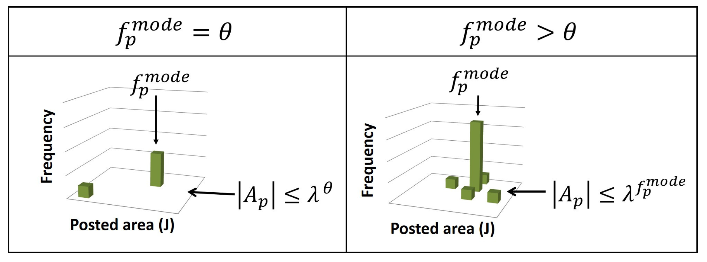
T h l determines the maximum number of sub-areas the geospatial tags w p can be used according to f p m o d e . As shown in Figure 2, the maximum number of sub-areas λ f p m o d e should be larger as f p m o d e gets higher, so that the tags used in multiple sub-areas can be extracted as long as they are used by sufficient number of users in one of the sub-areas. Here, by considering f p m o d e = θ as the lowest peak to determine the geospatial concept, we set T h l based on the maximum number of sub-areas λ θ when f p m o d e = θ as:
T h l = θ × l o g ( J / λ θ ) .
Setting θ low enables us to extract infrequently posted geospatial concepts as long as its spatial locality is high. Then, λ f p m o d e is determined higher as f p m o d e gets higher as:
λ f p m o d e = J exp T h l f p m o d e .
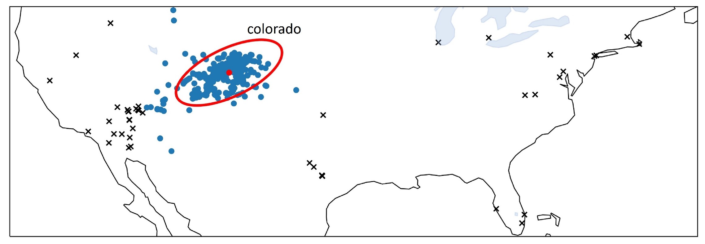
Each geospatial concept w p V g e o is associated with a set of geographical coordinates L p = { l n | w p W n } , as the locations where w p is captured. Since the images uploaded to Flickr can be associated with irrelevant tags, L p can also contain noise. Thus, we apply Mean Shift clustering algorithm [46] to L p to find the unknown number of local maximum or modes in the point distribution, which are potential cluster centers. Since the points associated with each local mode form a cluster, small clusters can be deleted as noise and the bivariate normal distribution is fitted to the set of points forming each remaining cluster as shown in Figure 3, to obtain the means and covariance matrices as the geospatial features of w p .

3.2. Visual Concept Extraction

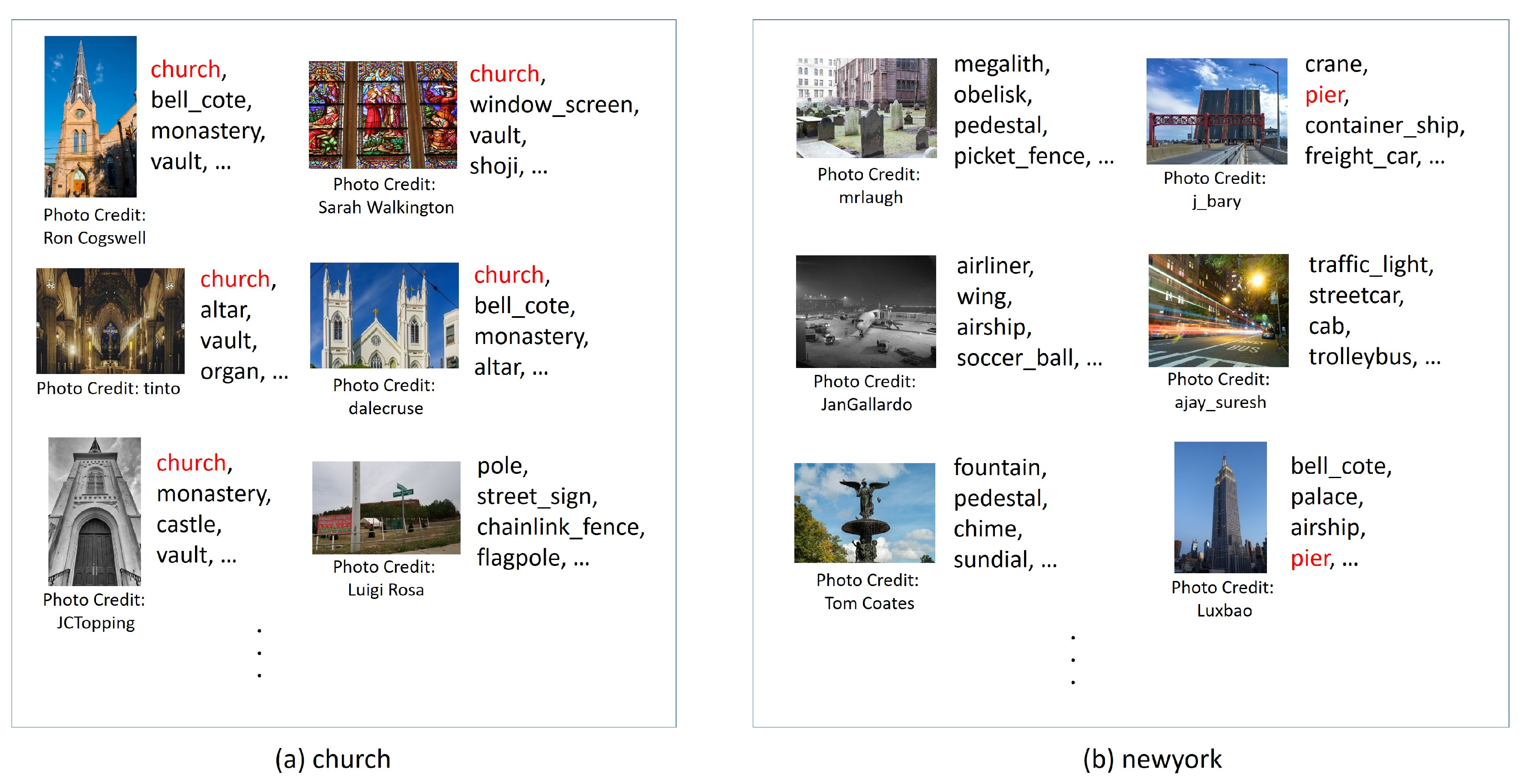
In order to extract the visual concepts, we examine the visual similarity among the images attached with each tag as the measure of its visual uniformity. For each tag w p W , a set of images tagged with w p are collected as I p = { I n | w p W n } . Since how users capture an image of specific concept can vary rather largely, the visual similarity among the images in I p is determined based on if similar objects are captured in the images. We use Xception [22], a CNN pre-trained on a large collection of ImageNet images of 1000 categories, to obtain the top-M categories for each image I n I p . Then, the number of images which share the most frequent category is obtained as C p . If C p | I p | T h v , the visual similarity among the images in I p is considered sufficiently high to determine w p as a visual concept. Figure 4 shows an example. In Figure 4a, the most frequent category predicted for I p was church, and it was predicted for most of the images in I p , which makes the concept w p = church a visual concept. On the other hand, in Figure 4b, even the most frequent category predicted for I p , which is pier, is predicted for only a few images in I p , indicating the visual diversity in I p . Thus, the concept w p = newyork is determined as a non-visual concept.
As a result, V v i s = { w p | w p W C p | I p | T h v } is extracted as a visual concept set. For each w p V v i s , the M most frequent categories predicted for I p are retained as its visual features. While I p is expected to contain images irrelevant to w p , they can also be filtered out based on the number of common categories between the M most frequent categories for w p and the top-M categories predicted for the image.

3.3. Representative Visual Concept Extraction

The visual geospatial concepts, which are extracted both as geospatial concepts in Step (1) and as visual concepts in Step (2), should be the visually recognizable fine-grained geospatial concepts. The simplest way to recognize these concepts would be to train a visual-based classifier by using their example images. However, due to the long-tail characteristics of Flickr images, only a small number of example images tend to be collected for these concepts. Based on the assumption that these visual geospatial concepts such as churches at different locations are generally visually similar and are the subordinate concepts of a specific coarse-grained representative visual concept such as church, which tend to have many example images, we determine such representative visual concepts whose visual features can be transferred to multiple visual geospatial concepts. The classifiers can be trained only for a small number of representative visual concepts, and the subordinate visual geospatial concepts can be discriminated based on their locations.
In order to determine the representative visual concepts for each visual geospatial concept, we can examine its visual similarity to all other visual concepts; however, as the number of visual concepts can be very large, it would be unnecessarily costly. Further, the coarse-grained representative concepts should be not only visually similar, but also semantically related to the visual geospatial concept. Thus, we confine the search space only to the semantically related visual concepts. Here, when the images with the tag w p are often tagged also with the tag w q , w p is considered to be semantically related to w q .
Then, when the images with the tag w p are visually similar to the images with the tag w q , w p is considered to be visually similar to w q . We examine the visual similarity between w p and w q based on the common objects in the images I p or I q . Thus, the visual similarity between w p and w q is calculated by the ratio of common categories in their visual features, that is, M most frequent categories.
When w q is assigned to more images than w p , w q can be considered to be a parent concept of w p , which represents a more generic concept applicable to more images. Thus, for each visual geospatial concept w p V v g , a set of its parent concepts P p = { w q | w q V v i s | I p I q | > 1 t f q t f p s v ( w p , w q ) T h s v } is obtained, where t f p represents the number of users of the tag w p , which is calculated as t f p = j = 1 J f p j , and s v ( w p , w q ) represents the visual similarity between w p and w q . Then, for each parent concept w q in P p , its parent concepts are recursively obtained.
Finally, for each visual geospatial concept w p V v g , the furthest concept w r which are either directly or indirectly reachable from w p and visually similar to w p are determined as its representative visual concepts. By searching not only the visually similar concepts which co-occur with the visual geospatial concept itself, but also those which co-occur with its parent concepts recursively, coarse-grained concepts with more example images can be determined as its representative visual concepts. As a result, a set of visual relations among the geospatial concepts and their representative visual concepts is extracted as A = { ( w p , w r ) | w p V v g w r R p s v ( w p , w r ) T h s v w q P r , s v ( w p , w q ) < T h s v } , where R p is a set of nodes in V v i s which are reachable from w p . A set of representative visual concepts is then determined as V r e p = { w r | ( w p , w r ) A } .
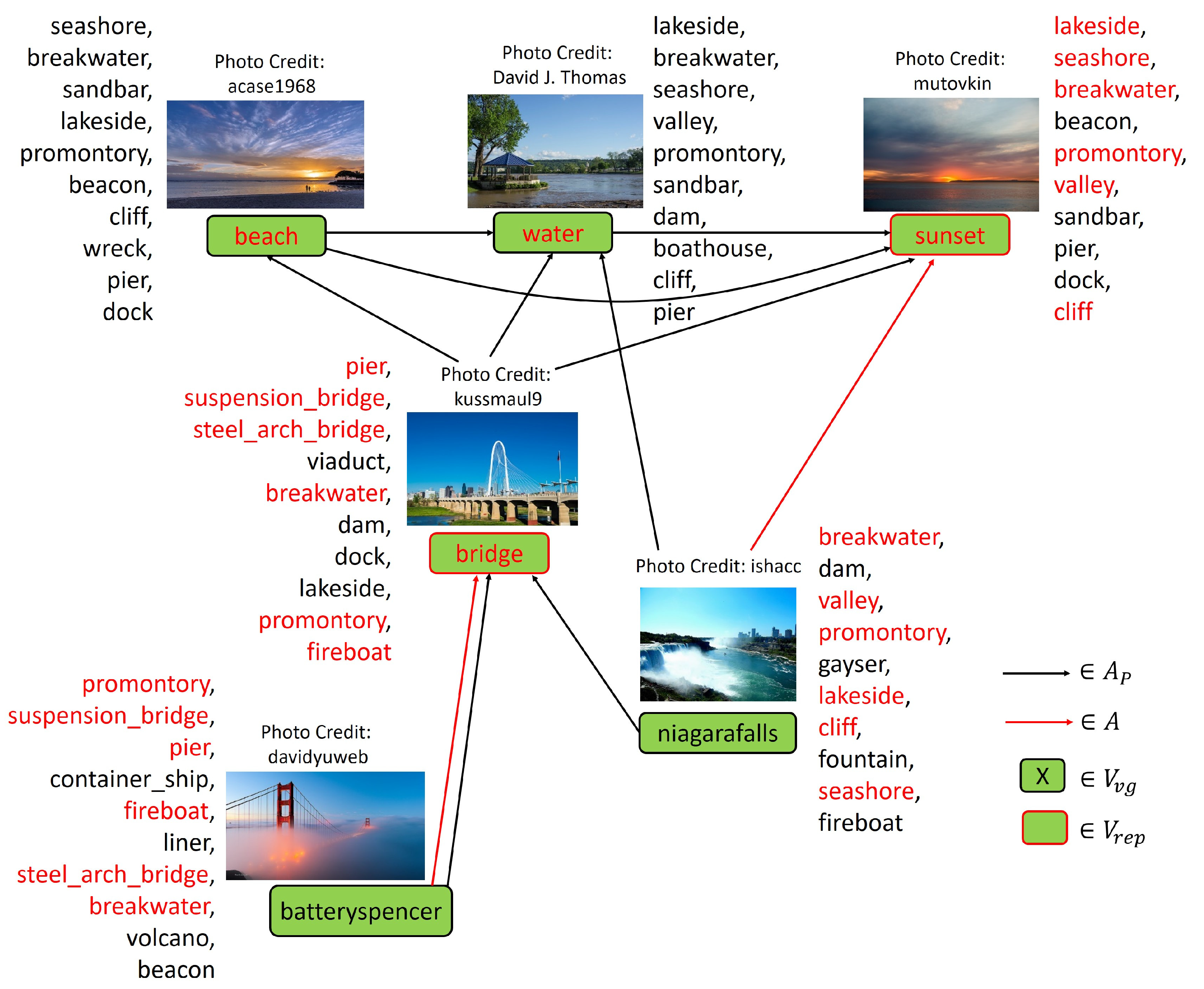
Figure 5 shows an example. Here, batteryspencer and niagarafalls are the visual geospatial concepts. The M = 10 most frequent categories predicted by CNN for each visual concept are shown with an example image. The black edges represent the semantically related and visually similar concept pairs when T h s v = 0.5 and are directed from each child to its parents. For each visual geospatial concept, the furthest either directly or indirectly reachable and visually similar concepts are determined as its representative visual concepts, which are indicated by red edges. The four visual concepts—bridge, beach, water, and sunset are all reachable both from batteryspencer and from niagarafalls. However, since only bridge is visually similar to batteryspencer ( s i m ( w p , w q ) T h s v ), bridge is determined as the representative visual concept of batteryspencer. On the other hand, all four visual concepts are visually similar to niagarafalls. Thus, the furthest concept sunset is determined as the representative visual concept of niagarafalls. The categories in red are the common categories between each pair of visual geospatial concept and its representative concept.

4. Experiments

4.1. Geospatial Concept Graph Construction from Flickr Images

We collected images captured in the United States in 2017 and attached at least one text tag from Flickr. As a result, 2,206,873 images uploaded by 28,945 users were collected. They were annotated with 22,339,112 text tags in total, among which 455,840 were unique. In order to check the spatial locality and visual uniformity of each tag, we only focused on the tags used at least by 5 users. As a result, the remaining 33,496 unique tags were used as a set of all tags W = n W n , from which geospatial and visual concepts are extracted to construct a geospatial concept graph.
Our proposed method has several parameters—the number of sub-areas J and T h l for extracting geospatial concepts, T h v for extracting visual concepts, and T h s v for examining the visual similarity between concepts. Here, we examined how changing the parameter values can affect the performance of our proposed method.
In order to evaluate the effects of the parameters J and T h l on the geospatial concept extraction, we have collected place names from a geographical database GeoNames [47] as the examples of geospatial concepts and stop words [48] as the examples of non-geospatial concepts. As discussed in Section 3.1, T h l can be determined by setting the maximum number of sub-areas λ θ in Equation (4) for determining a geospatial concept when f p m o d e = θ . Since the minimum number of users ( t f p ) of a tag w p is 5 as described above, we have set θ = 5 accordingly.
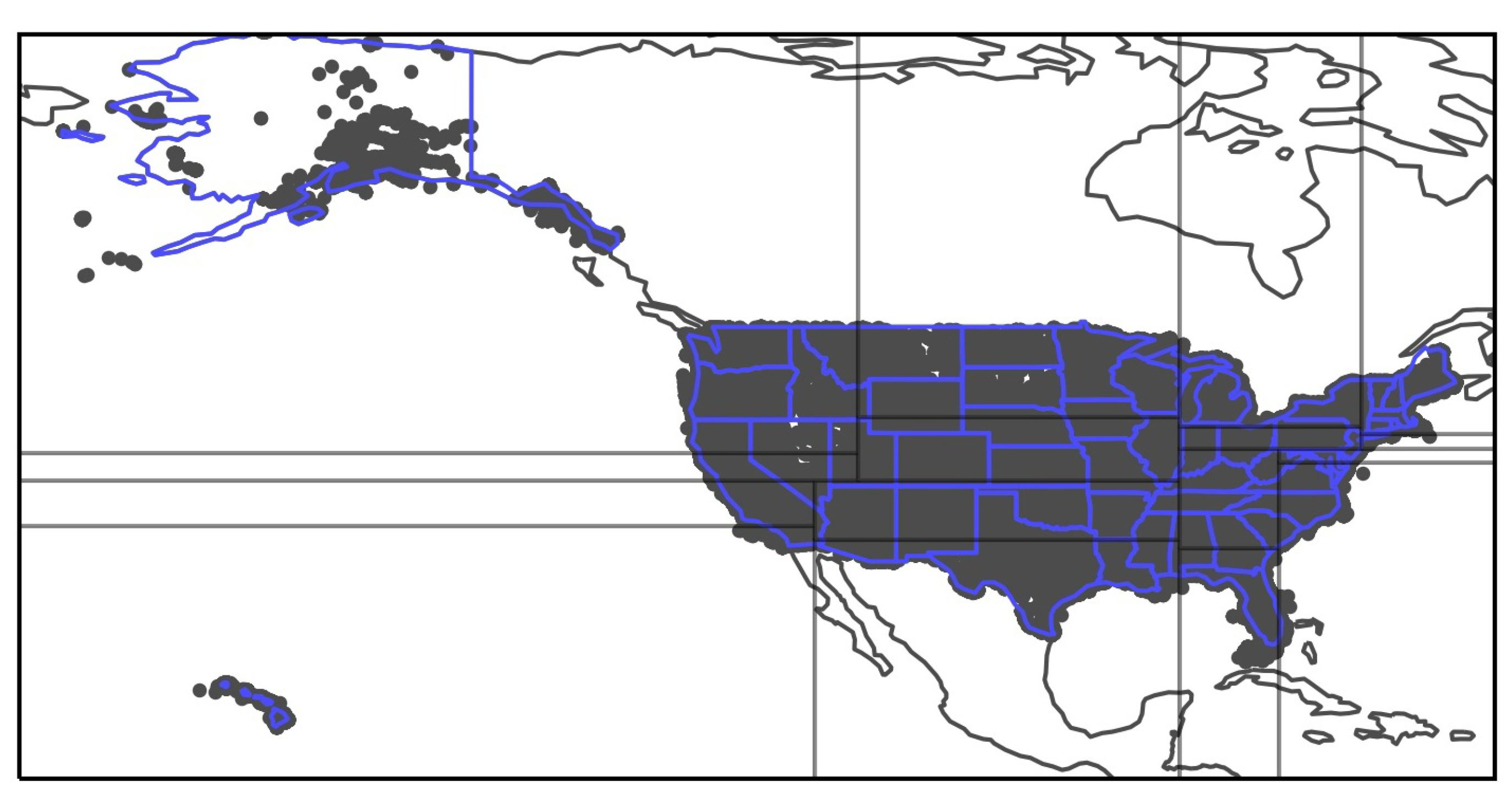
Table 1 shows the numbers of candidate place names and stop words which satisfy f p m o d e θ ( = 5 ) for different J. When J is set high, the locations of place names, especially the infrequently posted ones, can be separated into different sub-areas, making their locality unobservable. Further, dividing the area too much can make histograms sparse even for stop words; which resulted in their false extraction. However, setting J too low would increase f p m o d e for any word, which also resulted in the false extraction of stop words. λ θ should be also set higher to extract more place names, but setting it too high increased the false extraction of stop words. According to the results in Table 1, the best parameters were J = 16 and λ θ = 5 , which extracted the largest number of place names while extracting the fewest number of stop words. Figure 6 shows how the United Stated was divided when J = 16 .
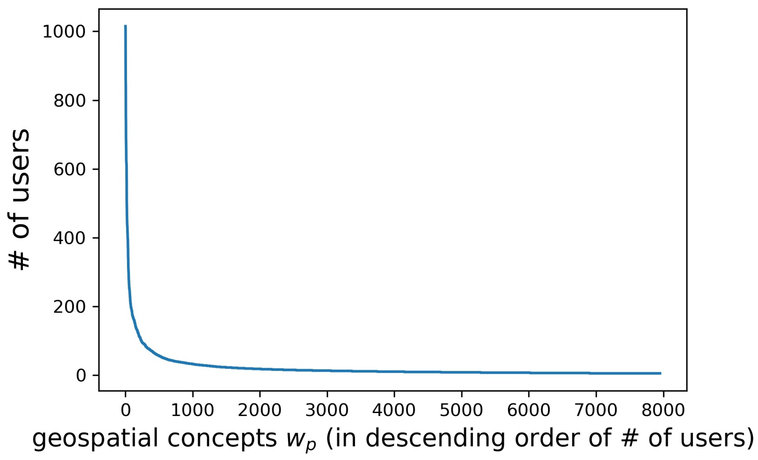
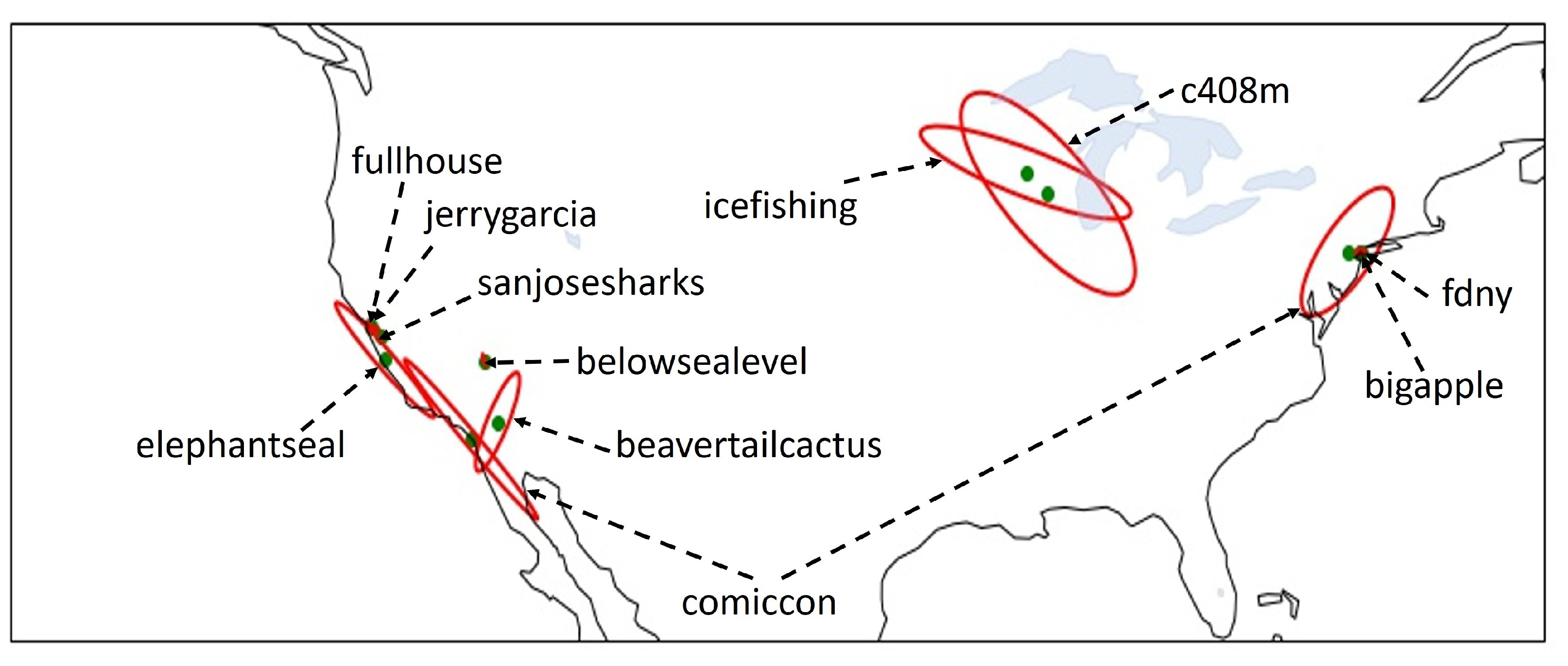
By setting J = 16 and λ θ = 5 , 7950 geospatial concepts were extracted from the 33,496 unique tags used in the United States in 2017. Figure 7 shows the number of users who used the extracted tags, where the tags are sorted in the descending order of the number of users. The frequency of the geospatial concepts in the Flickr images follows a long-tail distribution where only 3% of the geospatial concepts were used by more than 100 users. The geospatial concepts used by fewer than 25 users accounted for approximately 85% of geospatial concepts. 3299 of the extracted concepts were not in GeoNames, including acronyms such as fdny, nicknames such as bigapple, names of sports teams such as sanjosesharks, names of transportation systems such as c408m, names of iconic persons such as jerrygarcia, names of iconic locations such as fullhouse, names of events such as comiccon, local animals such as elephantseal, local plants such as beavertailcactus, local activities such as icefishing, and characteristics of areas such as belowsealevel. The bivariate normal distributions fitted to the geographical coordinates for these geospatial concepts are shown as the ellipses in Figure 8. Geospatial concepts indicating multiple locations were extracted such as comiccon. Their geospatial features are obtained as the means and covariance matrices of the distributions.
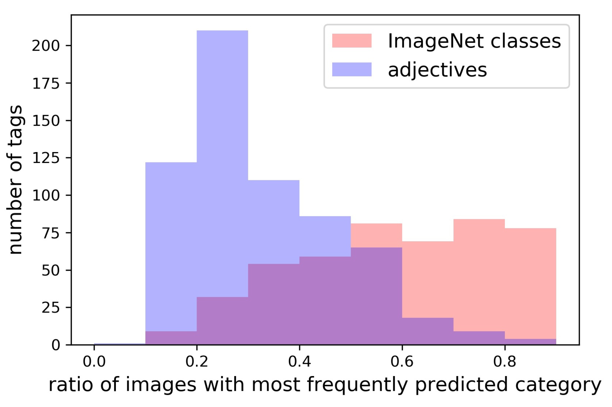
Further, in order to evaluate the effects of the parameters T h v to examine the uniformity of visual appearances of concepts, we have collected classes from ImageNet [25] as the examples of visual concepts and English adjectives as the examples of non-visual concepts, both of which are tagged to Flickr images. Figure 9 shows the distributions of the ratios of the images attached with most frequent category C p | I p | for each type of concepts when M = 10 . Accordingly, we set T h v = 0.5 . The ratio is over T h v = 0.5 for 70% of ImageNet classes, while the ratio is under T h v = 0.5 for 85% of adjectives.
By setting T h v = 0.5 , 16,620 visual concepts were extracted from the 33,496 unique tags used in the United States in 2017. 4617 out of the 7950 extracted geospatial concepts were also visual concepts, which are considered as visually recognizable fine-grained concepts. The distribution of the number of users for these visual geospatial concepts were similar to Figure 7, and less than 2% of them were used by more than 100 users.
Semantically related concept pairs are extracted based on their co-occurrence frequencies. We focus on the pairs of tags which were used together at least by 2 users by considering their credibility. In order to examine the effects of the parameters T h s v to examine the visual similarity between concepts, we have collected visually similar and semantically related concept pairs from GeoNames. Place names in GeoNames have feature codes which represent their place categories. As the examples of visual concepts, we have selected 4 place categories—‘MT’(mountain), ‘AIRP’(airport), ‘CH’(church), and ‘BDG’(bridge). Place names with these feature codes, which are also among the extracted visual concepts, are paired up with their corresponding tags—mountain, airports, church, and bridge. These pairs are used as the examples of visually similar concept pairs. On the other hand, for each of the tags corresponding to the place categories, we randomly paired it up with the extracted visual concepts and used them as the examples of visually dissimilar concept pairs. Figure 10 shows the distributions of visual similarities among the visually similar or dissimilar concept pairs. Setting T h s v = 0.5 would reject 90% of visually dissimilar concept pairs, while keeping about 70% of visually similar ones.
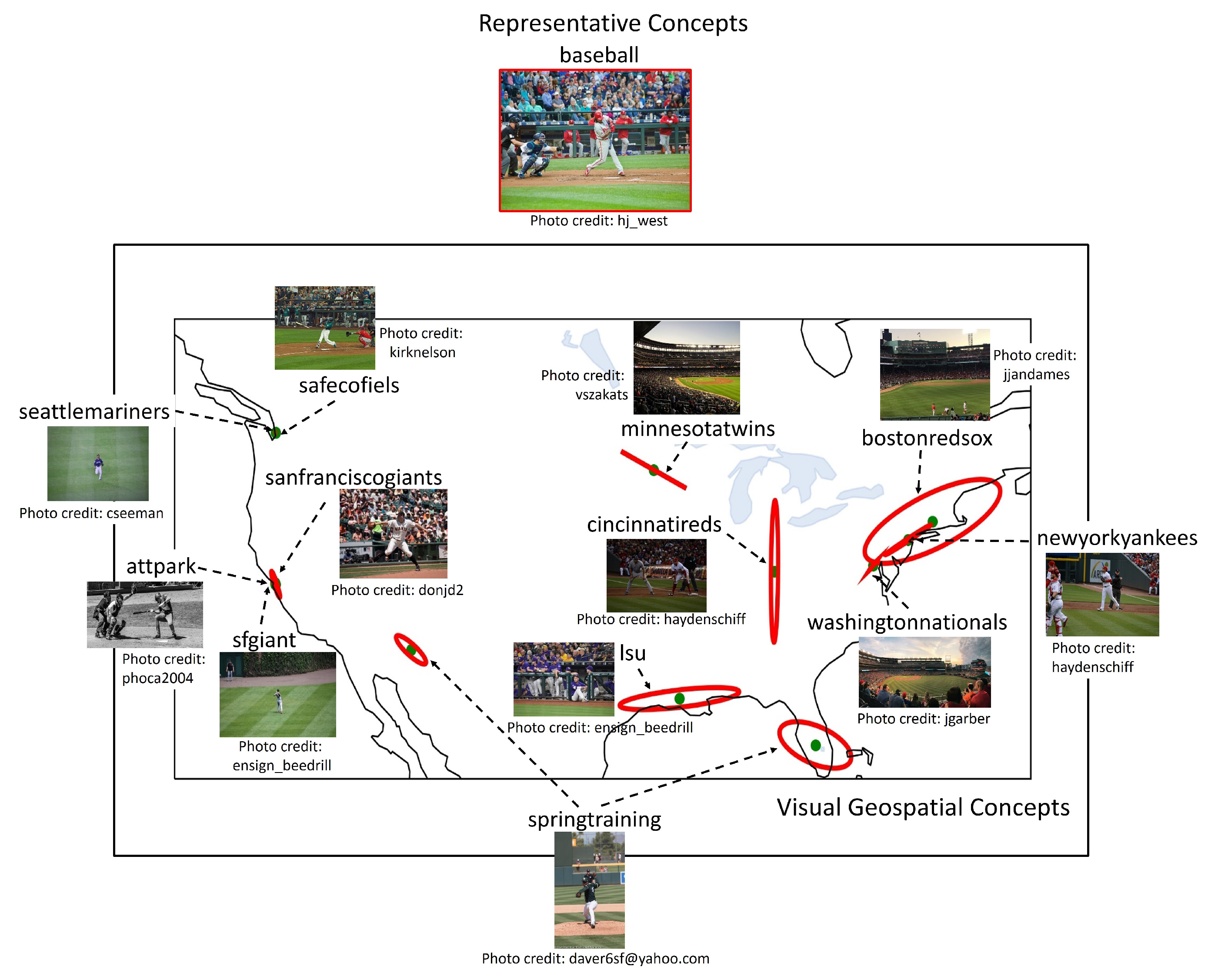
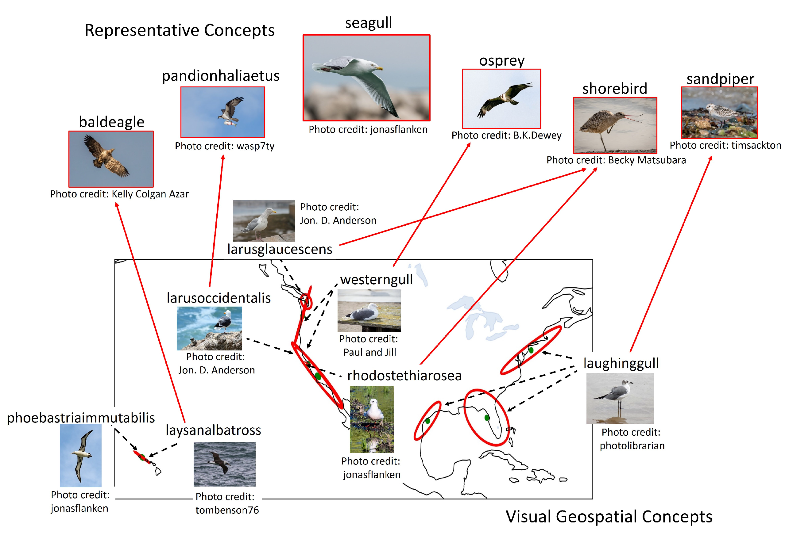
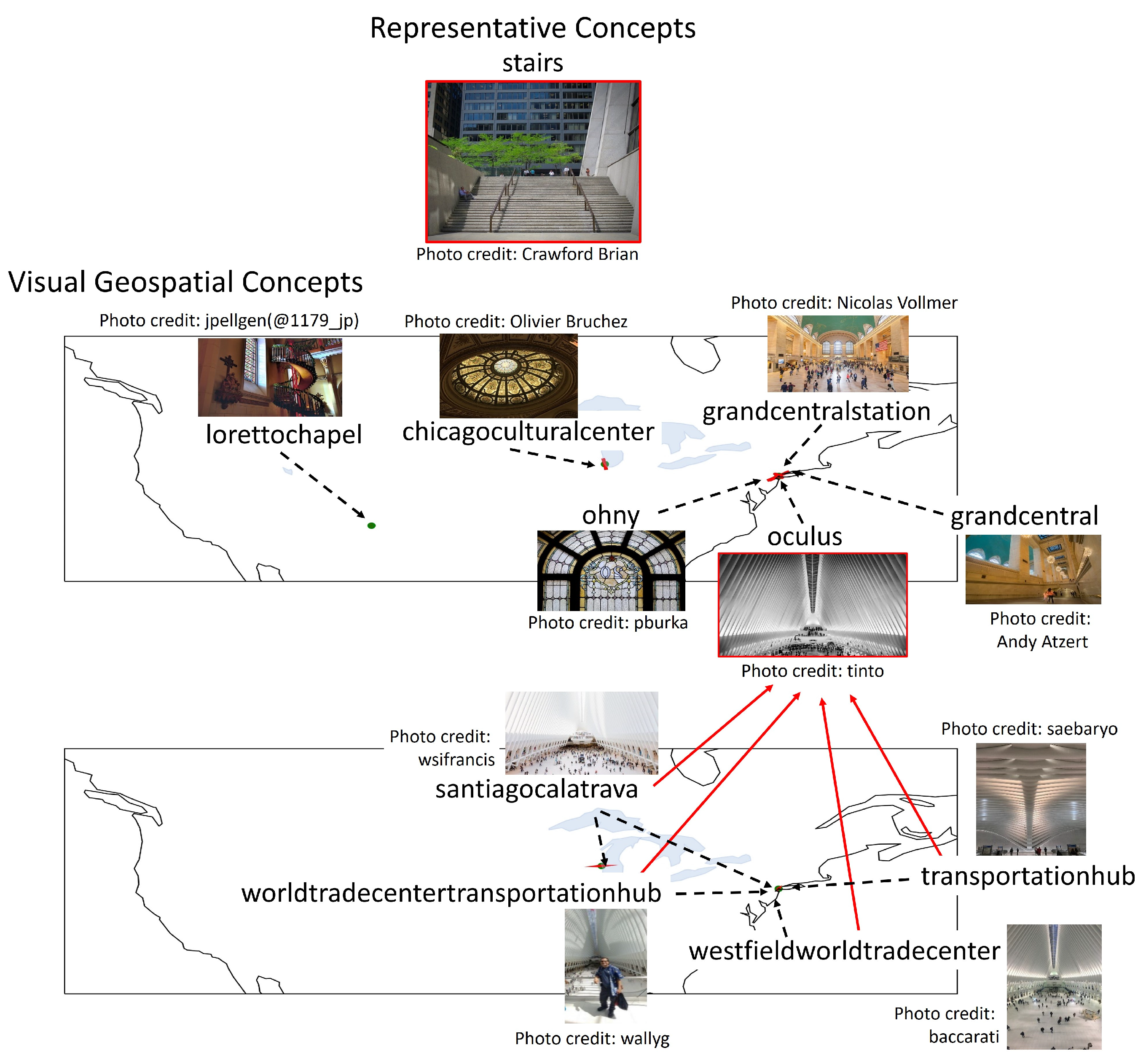
By setting T h s v = 0.5 , for the 3812 out of the 4617 visual geospatial concepts, 426 representative visual concepts were selected from the 16,620 visual concepts. Figure 11, Figure 12 and Figure 13 show the examples of the selected representative visual concepts and the visual geospatial concepts they represent. These figures also show an example image selected for each concept after filtering out the noisy images. The images surrounded by red rectangles represent the representative visual concepts. Some visual geospatial concepts can have multiple representative visual concepts as shown in Figure 12 and even visual geospatial concepts can be the representative visual concepts of other visual geospatial concepts as shown in Figure 13.

4.2. Evaluation by Geo-Aware Image Recognition

Although we have described the constructed geospatial concept graph with some examples, it is difficult to directly evaluate its quality. Thus, we evaluate its quality based on the performance of geo-aware image recognition. Here, we set the goal as, given an image I x captured at the location l x = ( l a t x , l o n x ) , to automatically obtain a list of its relevant visual geospatial concept tags W x = ( w p | w p V v g ) .
There can be many ways to use the constructed graph for geo-aware image recognition; however, we take a simple approach. When given an image I x captured at the location l x , the probability of assigning the visual geospatial concept w p as its tag can be written as:
P ( w p | I x , l x ) = P ( I x , l x | w p ) P ( w p ) P ( I x , l x ) .
Assuming that the image and location are conditionally independent given the visual geospatial concept, and each concept tag w p is equally assignable, we obtain:
P ( w p | I x , l x ) P ( I x | w p ) P ( l x | w p ) .
Since 426 representative visual concepts w r V r e p are expected to represent the 4617 visual geospatial concepts w p V v g , we use P ( I x | w r ) instead of P ( I x | w p ) as:
P ( w p | I x , l x ) m a x w r R p P ( I x | w r ) P ( l x | w p ) .
Thus, we only need to calculate P ( I x | w r ) for the 426 representative visual concepts w r V r e p . We determine P ( I x | w r ) , the probability of observing I x as the image of w r , based on the similarity of the visual features between I x and w r . For the image I x , the top-M categories is predicted by Xception, and the similarity between I x and the visual concept w r is obtained as the ratio of common categories between the top-M categories for I x and the M most frequent categories predicted for w r .
On the other hand, P ( l x | w p ) , the probability of observing l x as the location of the geospatial concept w p , can be determined based on the closeness of l x to the geospatial features of w p . More concretely, given a normal distribution with the mean and covariance matrix which were determined as the geospatial features of w p , the deviation of l x from the mean is calculated and the probability of observing the points outside the deviation is obtained as P ( l x | w p ) , so that P ( l x | w p ) is closer to 1 or 0 when l x is closer to or farther from the mean, respectively. Practically, P ( l x | w p ) needs to be calculated only for w p , which is the subordinate concept of w r such that P ( I x | w r ) > 0 .
We separately collected Flickr images captured in 2016 in the United States, each of which was attached with at least one of the visual geospatial concept tags w p V v g , as a set of test images. After removing images taken by the same users on the same days, which are often near-duplicate images, we obtained 71,258 test images in total. Although the tags which were actually attached to these images can be considered as the ground truth of the image recognition, these tags are not exhaustive. Thus, for each test image I x captured at l x , we ranked all w p for which P ( w p | I x , l x ) > = 0.001 in the order of P ( w p | I x , l x ) . Then, the results are evaluated with the recall rate, which is the ratio of the number of images correctly recognized as w p to the number of images to which w p was actually attached, and the ranks of w p . In order to properly evaluate the recall rate, we targeted the 3585 out of the 4617 visual geospatial concepts w p in the constructed graph, each of which was attached to at least 5 test images and examined whether the test images can be correctly recognized as the corresponding concepts.
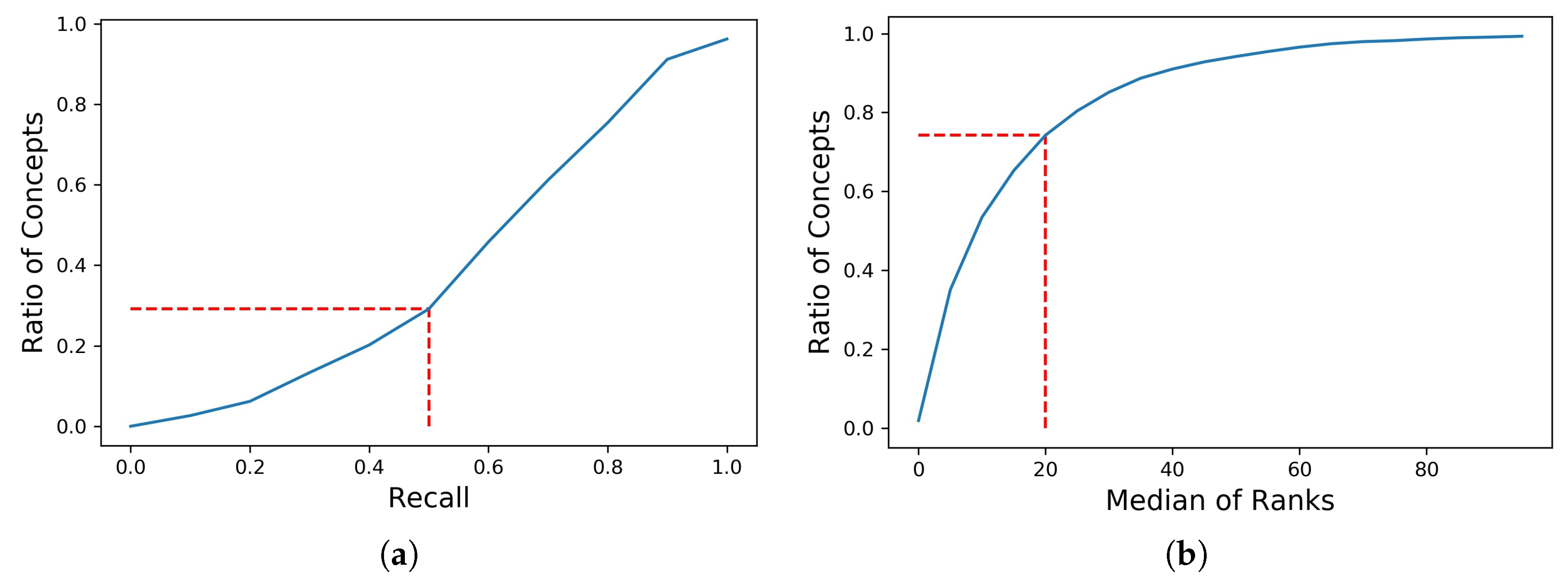
Figure 14a shows the distribution of the recall rates for the 3585 visual geospatial concepts. The recall rates were over 50% for 71% of the visual geospatial concepts. Figure 14b shows the cumulative distribution of median ranks of the corresponding tags w p for the correctly recognized images. For 74% of the concepts, the corresponding tags were ranked within the top 20 out of all the 3585 candidate tags.
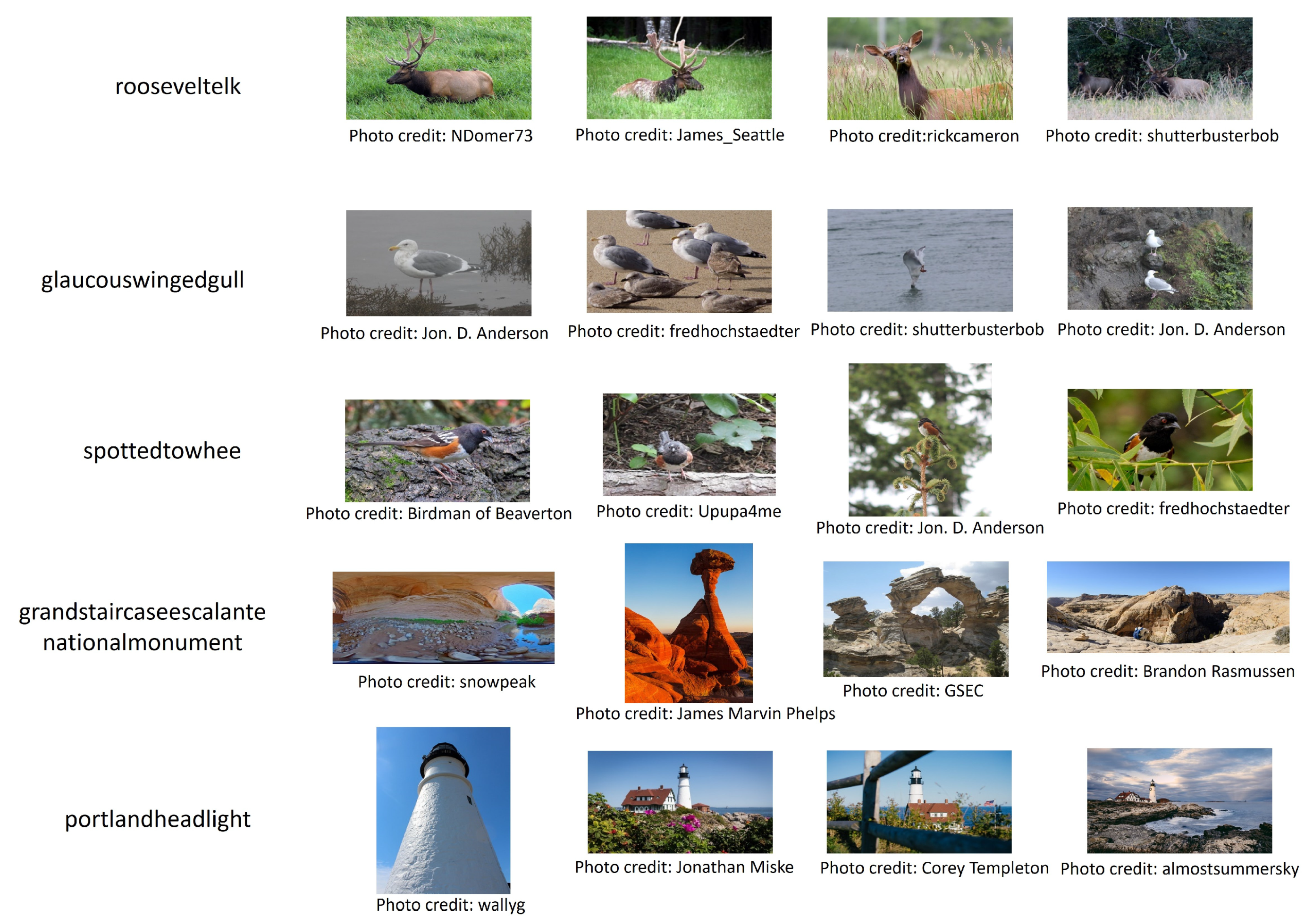
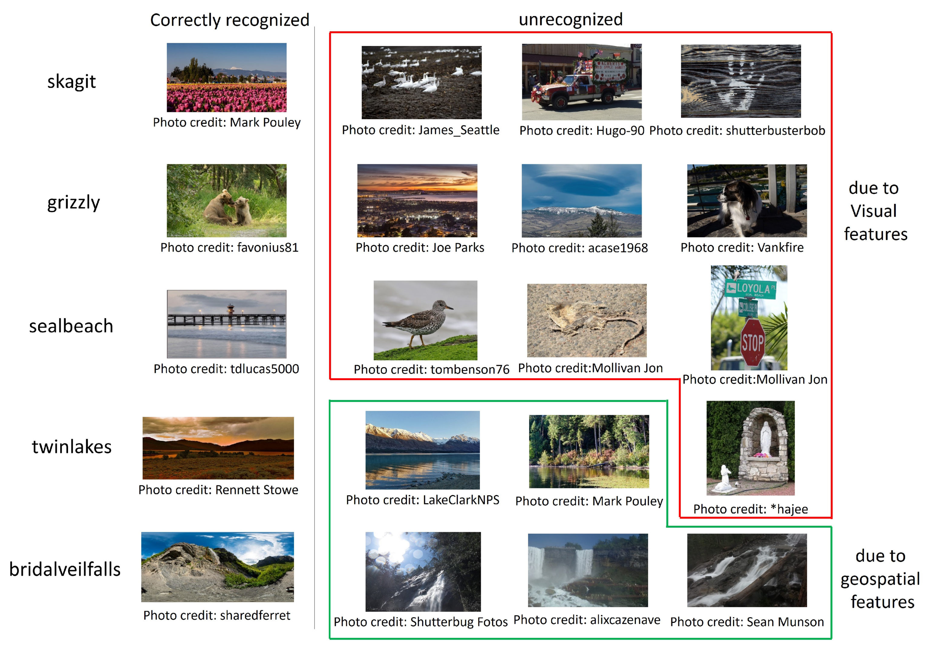
Figure 15 shows examples of the visual geosptial concepts with high recall rates. For diverse types of visual geospatial concepts, the test images attached with corresponding tags were correctly recognized despite their visual diversity. Further, Figure 16 shows examples of visual geospatial concepts with the recall rates of less than 50%. The leftmost images are the examples of correctly recognized images, and images on the right are the examples of unrecognized images. The images surrounded in red and green lines were determined dissimilar to the corresponding visual geospatial concepts based on visual and geospatial features, respectively. As can be seen, many of these incorrectly recognized images seem to be actually irrelevant to the corresponding geospatial concepts. Even when their visual appearances are similar as the images in the green lines, they can capture different concepts at locations which largely differ from where the corresponding geospatial concepts were observed in 2017. These results also indicate the existence of noise in the manually attached tags in Flickr and our geo-aware image recognition using the constructed graph was actually able to filter out such images with irrelevant tags.
On the other hand, since Flickr images captured in a single year are not sufficient to construct a complete graph, our method failed to recognize some correct test images or falsely recognized some incorrect test images. For example, although there are multiple waterfalls called bridal veil falls in the United States, most images tagged with bridalveilfalls were captured in Yosemite National Park in California in 2017. The 2 test images for bridalveilfalls on the right in Figure 16 correspond to Niagara Falls in New York, which is also called bridal veil falls, and they were not correctly recognized since the constructed graph did not contain its locations as the geospatial features of bridalveilfalls. Especially for geospatial concepts which can be observed in rather wide areas such as animals or transportation systems such as trains and airplanes, the images captured in a single year were not sufficient to extract complete geospatial features. While representative visual concepts can complement the visual features for their subordinate fine-grained geospatial concepts, the geospatial features need to be complemented from other information sources.
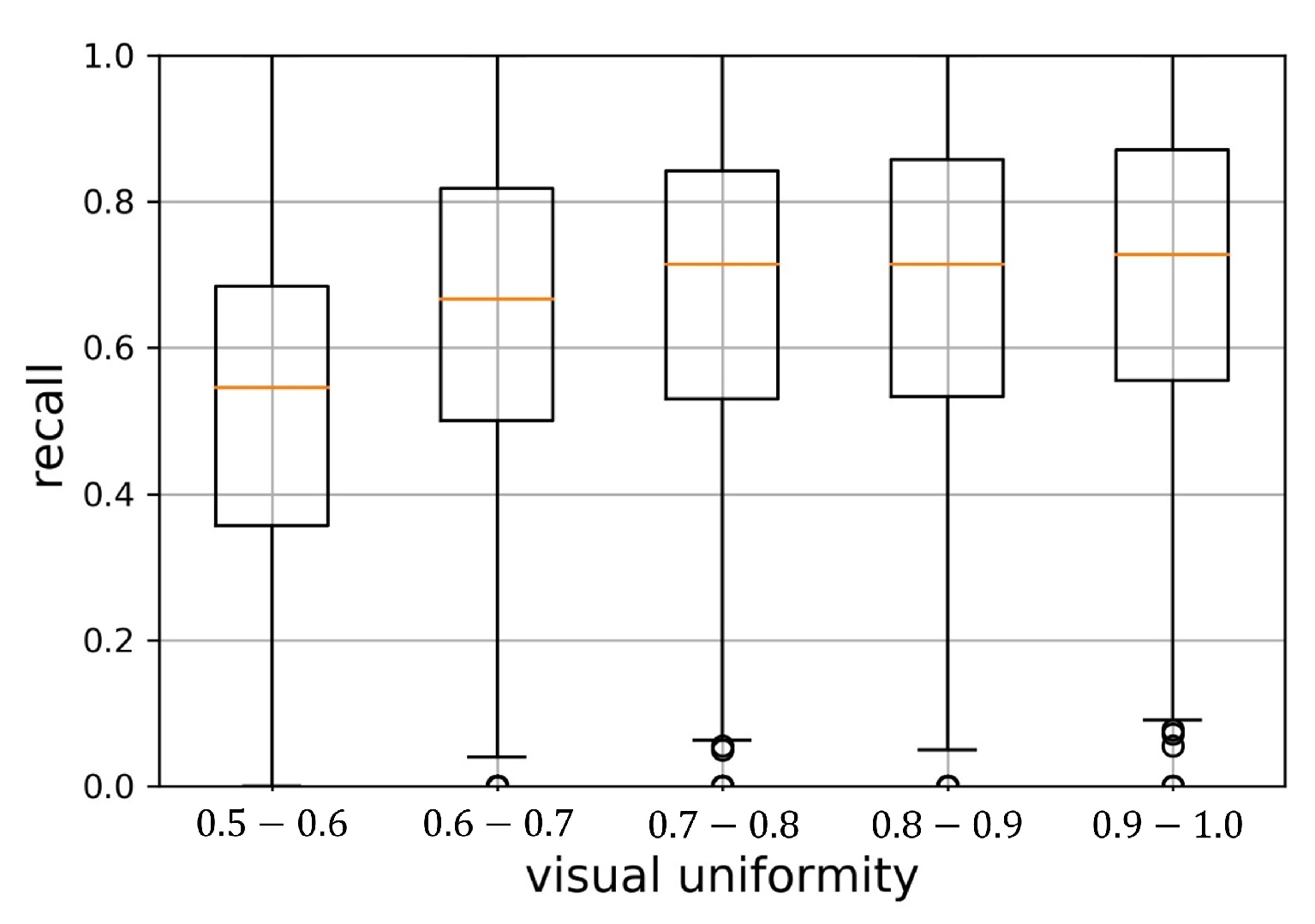
In addition, geospatial concepts such as names of towns whose actual visual appearances are diverse can be falsely extracted since visually similar images happened to be captured in 2017. Further, the noise images can hinder the extraction of proper visual features. The visual uniformity of such cases was relatively low and the images captured in 2016 were often visually dissimilar to the images captured in 2017. This can be seen in the relations between the visual uniformity and the recall rate as shown in Figure 17. The recall rates degraded for visually less uniform geospatial concepts especially when the visual uniformity was less than 0.6. Thus, the constructed graph can be considered as a base graph, whose missing or incorrect information can further be corrected.
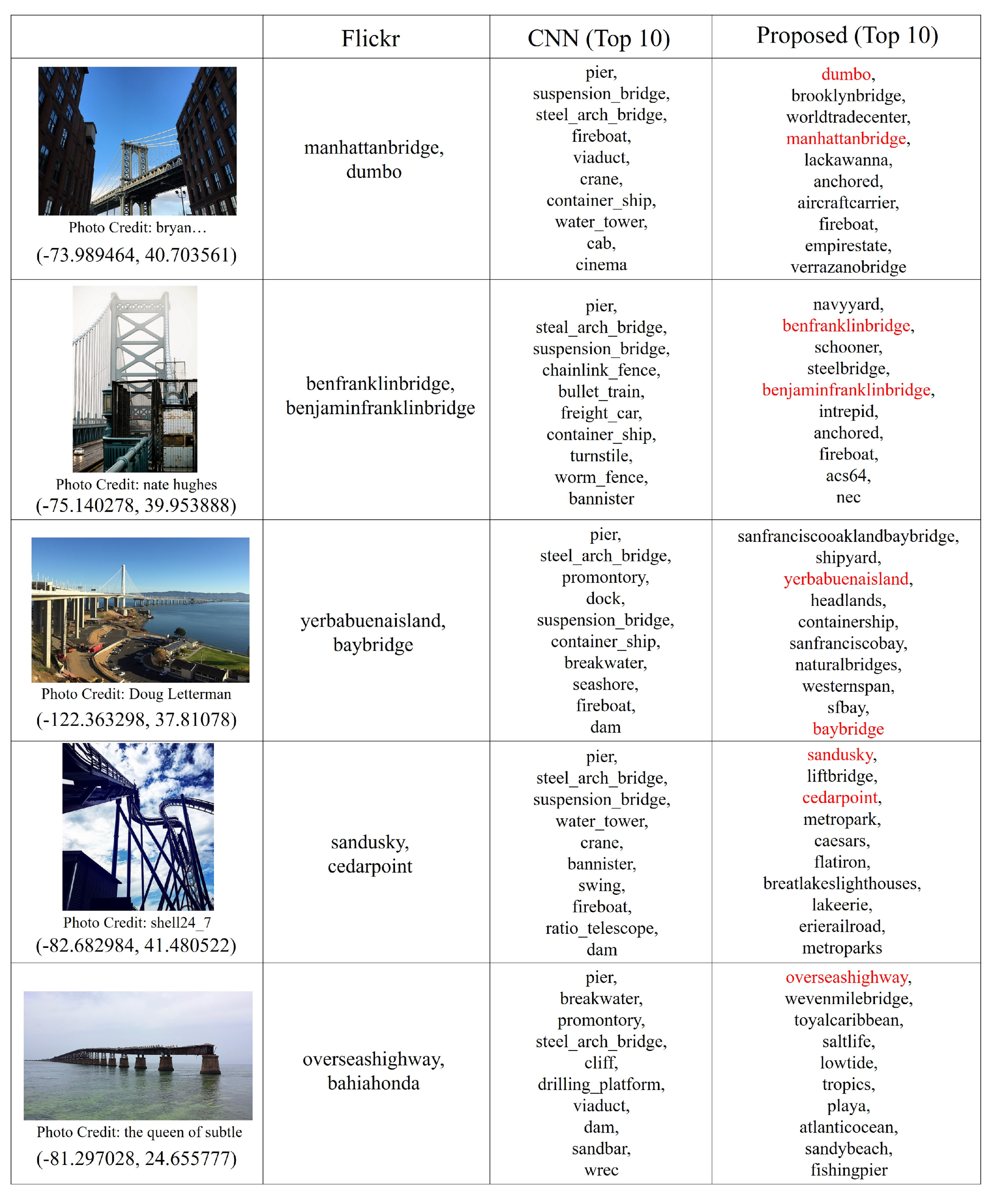
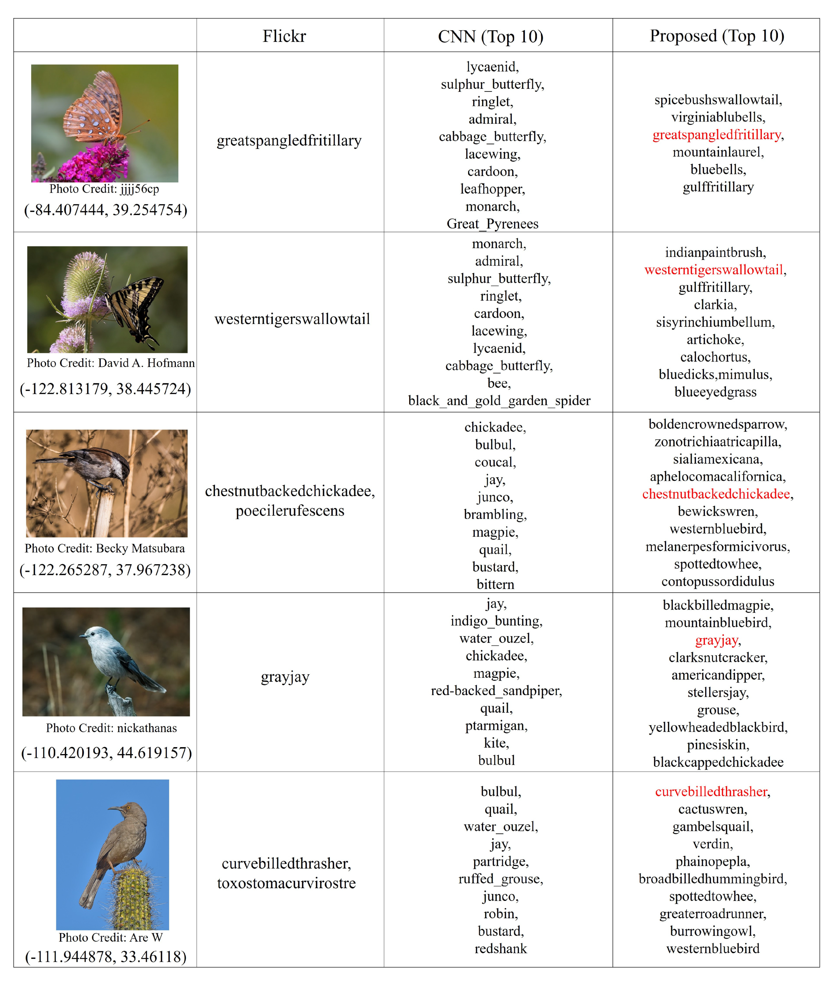
Although there is still a space for improvement, the constructed geospatial concept graph was able to realize the geo-aware fine-grained image recognition as shown in Figure 18 and Figure 19. By comparing the top 10 tags provided by our method with the Flickr tags, these figures show different fine-grained concepts were successfully recognized for the visually similar images captured at different locations. Further, visually dissimilar images captured at similar locations were also properly recognized. For example, the 3rd image in Figure 18 can also be recognized as westerntigerswallowtail or chestnutbackedchickadee, which were recognized for other images in Figure 19, based only on its captured location. However, based on the visual features, it was properly recognized as yerbabuenaisland or baybridge. The recognized geospatial concepts which are different from the Flickr tags can also be considered to be related to the test images, which also indicates the correctness of the information in the constructed geospatial concept graph.

5. Conclusions

The objective of this work is to increase the diversity of fine-grained geospatial concepts to which geo-aware fine-grained image recognition can be applied. Our assumption is that the images posted to image sharing services such as Flickr can be used to automatically provide the prior information about any type of fine-grained geospatial concepts that people would be interested in, as long as they are captured at specific locations by several people. Additionally, the problems with the Flickr images that most of the extracted fine-grained geospatial concepts would have only a limited number of example images to learn their visual features are expected to be solved by finding their representative visual concepts with more example images.
In order to achieve this objective, we proposed a method for automatically constructing a geospatial concept graph, which has the extracted prior knowledge in a structured way. The proposed method firstly extracts the fine-grained geospatial concepts by examining the spatial locality and visual uniformity of the posted images with each tag, and then extracts their representative visual concepts by examining the tag co-occurrence and the visual similarity among the extracted concepts.
The experimental results show that, from the 33,496 unique tags which were used at least by 5 users in a year in the United States in Flickr, our proposed method extracted 4617 visual geospatial concepts as the fine-grained geospatial concepts. Further, for the 3812 of these fine-grained concepts, 426 representative coarse-grained concepts were extracted, indicating the diversity of the domains of the extracted fine-grained geospatial concepts such as transportation systems (e.g., airplane, train, bus), living things (e.g., reptile, amphibian, butterfly, duck, eagle, tang fish, flower), architectures (e.g., bridge, castle, church, concert hall, raceway, sign, statue), landscapes (e.g., beach, mountain, river, trail), and sports teams (e.g., baseball).
The extracted prior information was used for the geo-aware image recognition for the test images captured in the United Stated in another year. The results have verified that the effectiveness of the proposed method in extracting the necessary information to be used for geo-aware fine-grained image recognition from Flickr images by recognizing more than 70% of the extracted fine-grained geospatial concepts with the recall rate of over 50%. Both the automatically extracted geospatial features and visual features transferred from the representative visual concepts were useful for discriminating closely-located visually dissimilar fine-grained geospatial concepts or distantly-located visually similar fine-grained geospatial concepts.
However, the bias or noise in the Flickr images can result in the insufficient information for the extracted concepts or the extraction of false information. Further, the diversity of the fine-grained geospatial concepts depend on the interest of Flickr users. For example, users do not often upload images of local food or product to Flickr. Thus, for practical applications which accurately recognizes much more diverse types of fine-grained geospatial concepts, we need to leverage more information sources not only Flickr images posted in a longer duration of time but also images posted to other image sharing or social networking services.
Although rather a simple approach was used for the geo-aware fine-grained image recognition to evaluate the quality of the constructed graph, the visual and geospatial feature-based recognizers/classifiers can be trained more properly with the collected images. Especially, the constructed geospatial concept graph can also be refined in the training process according to the recognition results so that the recognition accuracy would be improved. Devising such approaches would also be our future work.

Author Contributions

Conceptualization, Naoko Nitta; Methodology, Naoko Nitta; Software, Naoko Nitta; Validation, Naoko Nitta; Formal analysis, Naoko Nitta; Investigation, Naoko Nitta; Data curation, Naoko Nitta; Writing—original draft, Naoko Nitta; Writing—review and editing, Naoko Nitta, Kazuaki Nakamura, and Noboru Babaguchi. All authors have read and agreed to the published version of the manuscript.

Funding

This research was funded by Japan Society for the Promotion of Science KAKENHI: Grant Number 19K12019 and 16H06302.

Conflicts of Interest

The authors declare no conflict of interest. The founding sponsors had no role in the design of the study; in the collection, analyses, or interpretation of data; in the writing of the manuscript, and in the decision to publish the results.

References

  1. Wei, X.S.; Wu, J.; Cui, Q. Deep learning for fine-grained image analysis: A survey. arXiv 2019, arXiv:1907.03069. [Google Scholar]
  2. Berg, T.; Liu, J.; Woo Lee, S.; Alexander, M.L.; Jacobs, D.W.; Belhumeur, P.N. Birdsnap: Large-scale fing-grained visual categorization of birds. In Proceedings of the IEEE Conference on Computer Vision and Pattern Recognition, Columbus, OH, USA, 24–27 June 2014; pp. 2011–2018. [Google Scholar]
  3. Mac Aodha, O.; Cole, E.; Perona, P. Presence-only geographical priors for fine-grained image classification. In Proceedings of the IEEE International Conference on Computer Vision, Seoul, Korea, 27–28 October 2019; pp. 9596–9606. [Google Scholar]
  4. Chu, G.; Potetz, B.; Wang, W.; Howard, A.; Song, Y.; Brucher, F.; Leung, T.; Adam, H. Geo-aware networks for fine-grained recognition. In Proceedings of the IEEE International Conference on Computer Vision Workshops, Seoul, Korea, 27 October–2 November 2019. [Google Scholar]
  5. Van Horn, G.; Mac Aodha, O.; Song, Y.; Cui, Y.; Sun, C.; Shepard, A.; Adam, H.; Perona, P.; Belongie, S. The inaturalist species classification and detection dataset. In Proceedings of the IEEE Conference on Computer Vision and Pattern Recognition, Salt Lake City, UT, USA, 18–22 June 2018; pp. 8769–8778. [Google Scholar]
  6. Flickr. Available online: https://www.flickr.com/ (accessed on 26 May 2020).
  7. Sun, C.; Gan, C.; Nevatia, R. Automatic Concept Discovery from Parallel Text and Visual Corpora. In Proceedings of the IEEE International Conference on Computer Vision, Santiago, Chile, 11–18 December 2015; pp. 2596–2604. [Google Scholar]
  8. Chen, X.; Shrivastava, A.; Gupta, A. NEIL: Extracting visual knowledge from web data. In Proceedings of the IEEE International Conference on Computer Vision, Santiago, Chile, 11–18 December 2013; pp. 1409–1416. [Google Scholar]
  9. Learning everything about anything: webly-supervised visual concept learning. In Proceedings of the IEEE Conference on Computer Vision and Pattern Recognition, Columbus, OH, USA, 24–27 June 2014; pp. 3270–3277.
  10. Golge, E.; Duygulu, P. ConceptMap: mining noisy web data for concept learning. In Proceedings of the European Conference on Computer Vision, Zurich, Switzerland, 6–12 September 2014; pp. 439–455. [Google Scholar]
  11. Qiu, S.; Wang, X.; Tang, X. Visual semantic complex network for web images. In Proceedings of the IEEE International Conference on Computer Vision, Sydney, Australia, 1–8 December 2013; pp. 3623–3630. [Google Scholar]
  12. Tsai, D.; Jing, Y.; Liu, Y.; Rowley, H.A.; Ioffe, S.; Rehg, J.M. Large-scale image annotation using visual synset. In Proceedings of the IEEE International Conference on Computer Vision, Barcelona, Spain, 6–13 November 2011; pp. 611–618. [Google Scholar]
  13. Zhou, B.; Jagadeesh, V.; Piramuthu, R. ConceptLearner: discovering visual concepts from weakly labeled image collections. In Proceedings of the IEEE Conference on Computer Vision and Pattern Recognition, Boston, MA, USA, 7–12 June 2015; pp. 1492–1500. [Google Scholar]
  14. Moxley, E.; Kleban, J.; Manjunath, B. SpiritTagger: a geo-aware tag suggestion tool mined from Flickr. In Proceedings of the ACM International Conference on Multimedia Information Retrieval, Vancouver, BC, Canada, 30–31 October 2008; pp. 24–30. [Google Scholar]
  15. Silva, A.; Martins, B. Tag recommendation for georeferenced photos. In Proceedings of the ACM International Workshop on Location-Based Social Networks, San Diego, CA, USA, 30 November 2011; pp. 57–64. [Google Scholar]
  16. Liao, S.; Li, X.; Shen, H.T.; Yang, Y.; Du, X. Tag features for geo-aware image classification. IEEE Trans. Multimed. 2015, 17, 1058–1067. [Google Scholar] [CrossRef]
  17. Cui, Y.; Song, Y.; Sun, C.; Howard, A.; Belongie, S. Large scale fine-grained categorization and domain-specific transfer learning. In Proceedings of the IEEE Conference on Computer Vision and Pattern Recognition, Salt Lake City, UT, USA, 18–22 June 2018; pp. 4109–4118. [Google Scholar]
  18. Zhu, X.; Anguelov, D.; Ramanan, D. Capturing long-tail distributions of object subcategories. In Proceedings of the IEEE Conference on Computer Vision and Pattern Recognition, Columbus, OH, USA, 24–27 June 2014; pp. 915–922. [Google Scholar]
  19. Deng, J.; Ding, N.; Jia, Y.; Frome, A.; Murphy, K.; Bengio, S.; Li, Y.; Neven, H.; Adam, H. Large-scale object classification using label relation graphs. In Proceedings of the European Conference on Computer Vision, Zurich, Switzerland, 6–12 September 2014; pp. 48–64. [Google Scholar]
  20. Simonyan, K.; Zisserman, A. Very deep convolutional networks for large-scale image recognition. arXiv preprint 2014, arXiv:1409.1556. [Google Scholar]
  21. He, K.; Zhang, X.; Ren, S.; Sun, J. Deep residual learning for image recognition. In Proceedings of the IEEE Conference on Computer Vision and Pattern Recognition, Las Vegas, NV, USA, 27–30 June 2016; pp. 770–778. [Google Scholar]
  22. Chollet, F. Xecption: deep learning with depthwise separable convolutions. In Proceedings of the IEEE Conference on Computer Vision and Pattern Recognition, Honolulu, HI, USA, 21–26 July 2017; pp. 1251–1258. [Google Scholar]
  23. Szegedy, C.; Ioffe, S.; Vanhoucke, V.; Alemi, A.A. Inception-v4, inception-resnet and the impact of residual connections on learning. In Proceedings of the AAAI Conference on Artificial Intelligence, San Francisco, CA, USA, 4–9 February 2017; pp. 4278–4284. [Google Scholar]
  24. Huang, G.; Liu, Z.; Van Der Maaten, L.; Weinberger, K.Q. Densely connected convolutional networks. In Proceedings of the IEEE Conference on Computer Vision and Pattern Recognition, Honolulu, HI, USA, 21–26 July 2017; pp. 4700–4708. [Google Scholar]
  25. Deng, J.; Dong, W.; Socher, R.; Li, L.J.; Li, K.; Fei-Fei, L. ImageNet: a large-scale hierarchical image database. In Proceedings of the IEEE Conference on Computer Vision and Pattern Recognition, Miami, FL, USA, 20–25 June 2009; pp. 248–255. [Google Scholar]
  26. Zhou, B.; Lapedriza, A.; Xiao, J.; Torralba, A.; Oliva, A. Learning deep features for scene recognition using places database. In Proceedings of the Advances in Neural Information Processing Systems, Montreal, QC, Canada, 8–13 December 2014; pp. 487–495. [Google Scholar]
  27. Marino, K.; Salakhutdinov, R.; Gupta, A. The more you know: using knowledge graphs for image classification. In Proceedings of the IEEE Conference on Computer Vision and Pattern Recognition, Honolulu, HI, USA, 21–26 July 2017. [Google Scholar]
  28. Malisiewicz, T.; Efros, A. Beyond categories: the visual memex model for reasoning about object relationships. In Proceedings of the Advances in neural information processing systems, Vancouver, BC, Canada, 7–10 December 2009; pp. 1222–1230. [Google Scholar]
  29. Fang, Y.; Kuan, K.; Lin, J.; Tan, C.; Chandrasekhar, V. Object detection meets knowledge graphs. In Proceedings of the International Joint Conference on Artificial Intelligence, Honolulu, HI, USA, 21–26 July 2017; pp. 1661–1667. [Google Scholar]
  30. Zhang, D.; Cui, M.; Yang, Y.; Yang, P.; Xie, C.; Liu, D.; Yu, B.; Cheng, Z. Knowledge graph-based image classification refinement. IEEE Access 2019, 7, 57678–57690. [Google Scholar] [CrossRef]
  31. WordNet. Available online: https://wordnet.princeton.edu/ (accessed on 26 May 2020).
  32. DBpedia. Available online: https://wiki.dbpedia.org/ (accessed on 26 May 2020).
  33. Russell, B.C.; Torralba, A.; Murphy, K.P.; Freeman, W.T. LabelMe: a database and web-based tool for image annotation. Int. J. Comput. Vis. 2008, 77, 157–173. [Google Scholar] [CrossRef]
  34. Krishna, R.; Zhu, Y.; Groth, O.; Johnson, J.; Hata, K.; Kravitz, J.; Chen, S.; Kalantidis, Y.; Li, L.J.; Shamma, D.A.; et al. Visual genome: connecting language and vision using crowdsourced dense image annotations. Int. J. Comput. Vis. 2017, 123, 32–73. [Google Scholar] [CrossRef] [Green Version]
  35. Chen, T.; Lin, L.; Chen, R.; Wu, Y.; Luo, X. Knowledge-embedded representation learning for fine-grained image recognition. arXiv preprint 2018, arXiv:1807.00505. [Google Scholar]
  36. Xu, H.; Qi, G.; Li, J.; Wang, M.; Xu, K.; Gao, H. Fine-grained image classification by visual-semantic embedding. In Proceedings of the International Joint Conferences on Artificial Intelligence, Stockholm, Sweden, 13–19 July 2018; pp. 1043–1049. [Google Scholar]
  37. Krause, J.; Sapp, B.; Howard, A.; Zhou, H.; Toshev, A.; Duerig, T. The unreasonable effectiveness of noisy data for fine-grained recognition. In Proceedings of the European Conference on Computer Vision, Amsterdam, The Netherlands, 11–14 October 2016; pp. 301–320. [Google Scholar]
  38. Papadopoulos, S.; Zigkolis, C.; Kompatsiaris, Y.; Vakali, A. Cluster-based landmark and event detection for tagged photo collections. IEEE Multimed. 2010, 52–63. [Google Scholar] [CrossRef]
  39. Zheng, Y.T.; Zhao, M.; Song, Y.; Adam, H.; Buddemeier, U.; Bissacco, A.; Brucher, F.; Chua, T.S.; Neven, H. Tour the world: building a web-scale landmark recognition engine. In Proceedings of the IEEE Conference on Computer Vision and Pattern Recognition, Miami, FL, USA, 20–25 June 2009; pp. 1085–1092. [Google Scholar]
  40. Crandall, D.J.; Backstrom, L.; Huttenlocher, D.; Kleinberg, J. Mapping the world’s photos. In Proceedings of the International Conference on World Wide Web, Madrid, Spain, 20–24 April 2009; pp. 761–770. [Google Scholar]
  41. Tang, K.; Paluri, M.; Fei-Fei, L.; Fergus, R.; Bourdev, L. Improving image classification with location context. In Proceedings of the IEEE International Conference on Computer Vision, Santiago, Chile, 11–18 December 2015; pp. 1008–1016. [Google Scholar]
  42. Rattenbury, T.; Naaman, M. Methods for extracting place semantics from Flickr tags. ACM Trans. Web 2009, 3, 1–30. [Google Scholar]
  43. Zheng, X.; Han, J.; Sun, A. A survey of location prediction on Twitter. IEEE Trans. Knowl. Data Eng. 2018, 30, 1652–1671. [Google Scholar] [CrossRef] [Green Version]
  44. Lim, J.; Nitta, N.; Nakamura, K.; Babaguchi, N. Constructing geographic dictionary from streaming geotagged tweets. ISPRS Int. J. -Geo-Inf. 2019, 8, 216. [Google Scholar] [CrossRef] [Green Version]
  45. Roller, S.; Speriosu, M.; Rallapalli, S.; Wing, B.; Baldridge, J. Supervised text-based geolocation using language models on an adaptive grid. In Proceedings of the Joint Conference on Empirical Methods in Natural Language Processing and Computational Natural Language Learning, Jeju Island, Korea, 12–14 July 2012; pp. 1500–1510. [Google Scholar]
  46. Comaniciu, D.; Meer, P. Mean shift: A robust approach toward feature space analysis. IEEE Trans. Pattern Anal. Mach. Intell. 2002, 24, 603–619. [Google Scholar] [CrossRef] [Green Version]
  47. GeoNames. Available online: http://www.geonames.org/ (accessed on 26 May 2020).
  48. Stopwords ISO. Available online: https://github.com/stopwords-iso/stopwords-iso (accessed on 26 May 2020).
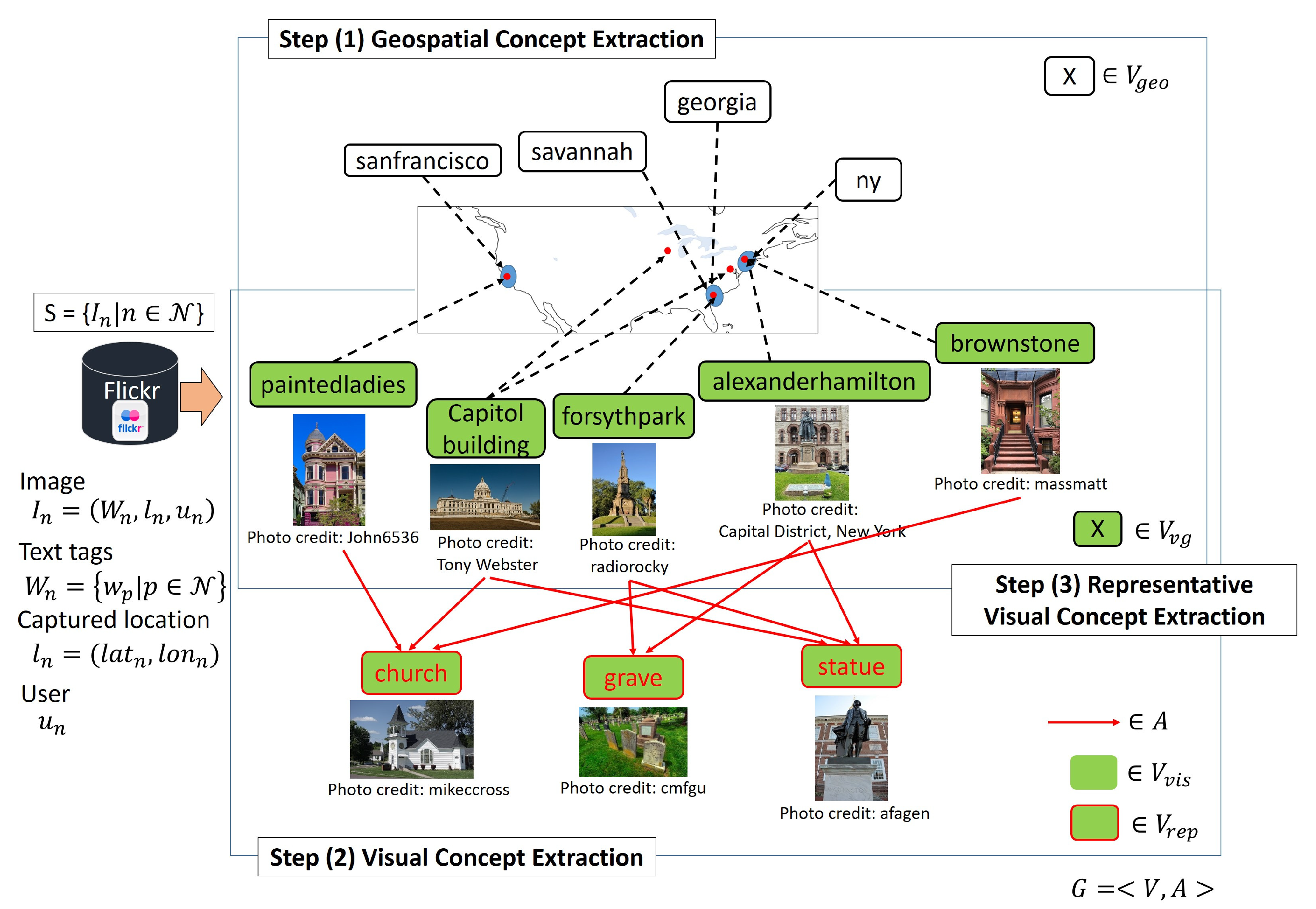
Figure 1. Overview of Proposed Method
Ijgi 09 00354 g001
Figure 2. How the area-based frequency histogram F p is used to determine if w p represents a geospatial concept. Intuitively, by using the same threshold T h l , the threshold λ f p m o d e which represents the maximum number of sub-areas for extracting the geospatial concepts gets larger as the peak f p m o d e of the frequency histogram gets higher.
Ijgi 09 00354 g002
Figure 3. How geospatial features of geospatial concepts are obtained by applying Mean Shift clustering to L p when w p = colorado . Cross marks represent the removed l n and blue marks represent the points l n forming a cluster. The red ellipse represents the 95% confidence interval based on the mean and covariance matrix of the bivariate normal distribution fitted to the blue marks.
Ijgi 09 00354 g003
Figure 4. Examples of how the top categories predicted by CNN for each image in I p are used to determine if w p represents a visual concept. (a,b) each shows an example for visual concepts and non-visual concepts. The most frequent category predicted for each concept is shown in red. When M is set to 10, the 10 most frequent categories for (a) are church, monastery, bell_cote, vault, palace, dome, castle, altar, barn, and tile_roof, which filter out the bottom right image as irrelevant image.
Ijgi 09 00354 g004
Figure 5. Examples of how the representative visual concepts are determined. A P represented by black lines is a set of edges between each concept and its parent nodes. For each visual geospatial concept, the furthest either directly or indirectly reachable visually similar concepts, which are to be its representative visual concepts, are searched by using these edges.
Ijgi 09 00354 g005
Figure 6. How the United States was divided into J = 16 sub-areas. The dark circles represent the geographical coordinates of the 2,206,873 images. The whole area, which is the minimum bounding box containing all coordinates, is divided so that each sub-area has the same number of images.
Ijgi 09 00354 g006
Figure 7. Number of users for extracted geospatial concepts w p , where w p is ranked in the descending order of the number of users. Examples of the geospatial concepts used by more than 100 users are mostly names of states, big cities, or popular places such as manhattan, centralpark, chinatown, and hollywood.
Ijgi 09 00354 g007
Figure 8. Examples of extracted geospatial concepts which are not in GeoNames and their locations (means and covariance matrices) obtained as the geospatial features.
Ijgi 09 00354 g008
Figure 9. Ratio of images with most frequently predicted category for each concept.
Ijgi 09 00354 g009
Figure 10. Distributions of visual similarities for each type of concept pairs
Ijgi 09 00354 g010
Figure 11. Examples of visual geospatial concepts represented by a visual concept baseball. The edges among the visual geospatial concepts and baseball are omitted for visual clarity.
Ijgi 09 00354 g011
Figure 12. Examples of visual geospatial concepts represented by a visual concept seagull. They can be represented by multiple visually similar visual concepts. Only the edges among the visual geospatial concepts and visual concepts other than seagull are presented for visual clarity.
Ijgi 09 00354 g012
Figure 13. Examples of visual geospatial concepts represented by a visual concept stairs. The visual geospatial concepts themselves can also represent other visual geospatial concepts. The visual concept stairs represent the visual geospatial concepts shown in the middle layer: lorettochapel, chicagoculturalcenter, grandcentralstation, grandcentral, ohny, and oculus. oculus represents the visual geospatial concepts in the bottom layer. Only the edges among oculus and other visual geospatial concepts are presented for visual clarity.
Ijgi 09 00354 g013
Figure 14. The image recognition results when the recognition targets were the 3585 visual geospatial concepts w p which was actually attached to at least 5 test images. (a) Cumulative distribution of recall rates. (b) Cumulative distribution of median ranks.
Ijgi 09 00354 g014
Figure 15. Examples of geospatial concepts whose test images were all correctly recognized.
Ijgi 09 00354 g015
Figure 16. Examples of geospatial concepts whose test images were only partly correctly recognized.
Ijgi 09 00354 g016
Figure 17. Relations between visual uniformity C p | I p | and recall of geo-aware image recognition.
Ijgi 09 00354 g017
Figure 18. Examples of image recognition results for visually similar test images captured at different locations.
Ijgi 09 00354 g018
Figure 19. Examples of image recognition results for visually similar test images captured at different locations.
Ijgi 09 00354 g019
Table 1. Numbers of extracted place names and stop words for different parameters J and θ .
♯ of Sub-Areas J
8163264128256
♯ of candidate place names731267106236585955285229
♯ of candidate stop words14811886695338
4♯ of extracted place names468745294443438043134215
♯ of extracted stop words211232
5♯ of extracted place names493546714545447743884270
♯ of extracted stop words311332
λ θ 6♯ of extracted place names523747904616453644354322
♯ of extracted stop words1122333
7♯ of extracted place names556149154710460444994357
♯ of extracted stop words3322334