Modelling Housing Rents Using Spatial Autoregressive Geographically Weighted Regression: A Case Study in Cracow, Poland


Abstract
1. Introduction
- What factors significantly affect housing rents in Cracow?
- Is there spatial autocorrelation of rental prices?
- Is there spatial heterogeneity in relation to independent variables or to the spatial autoregressive term?
2. Literature Review on House and Rental Price Determinants
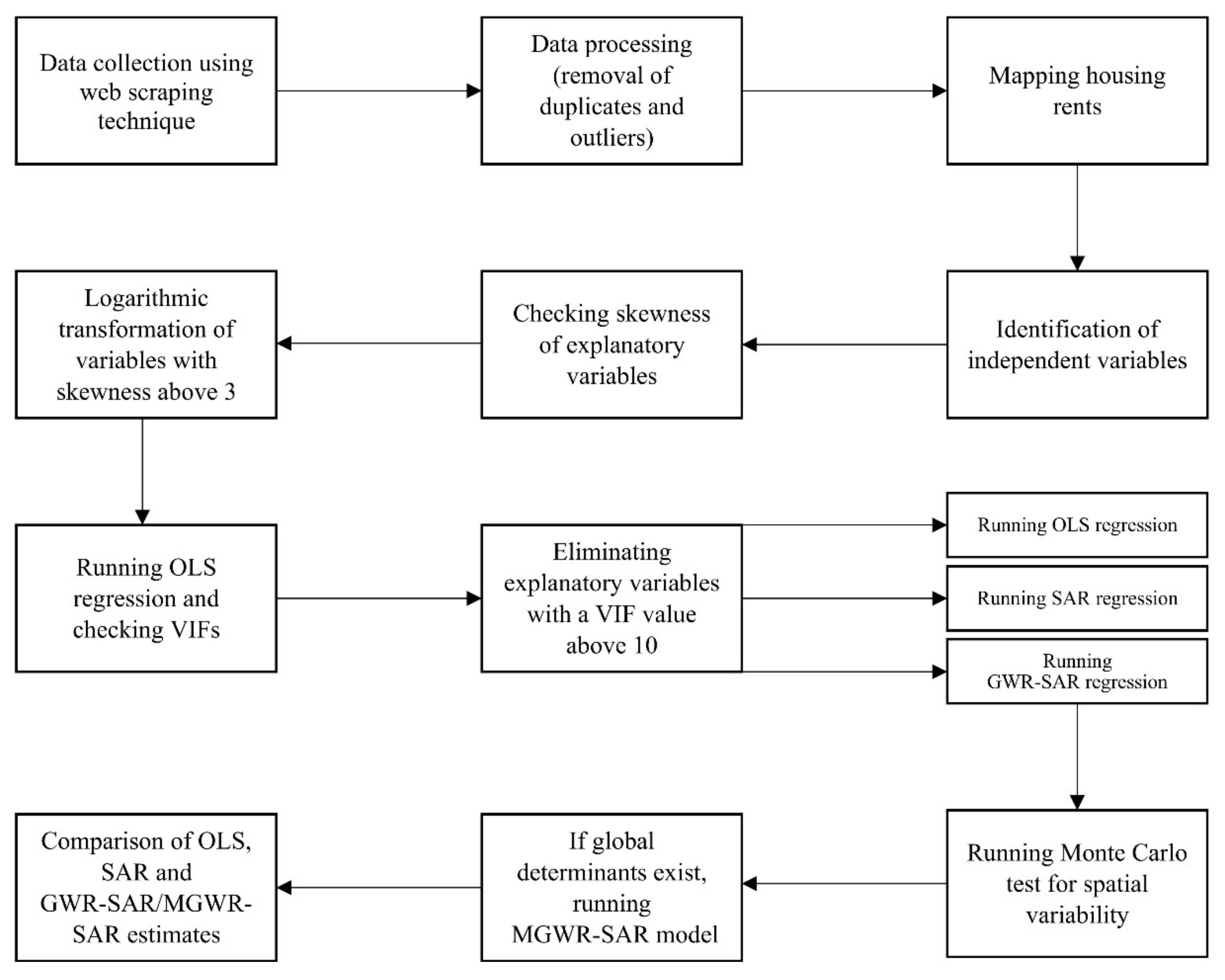
3. Methodology
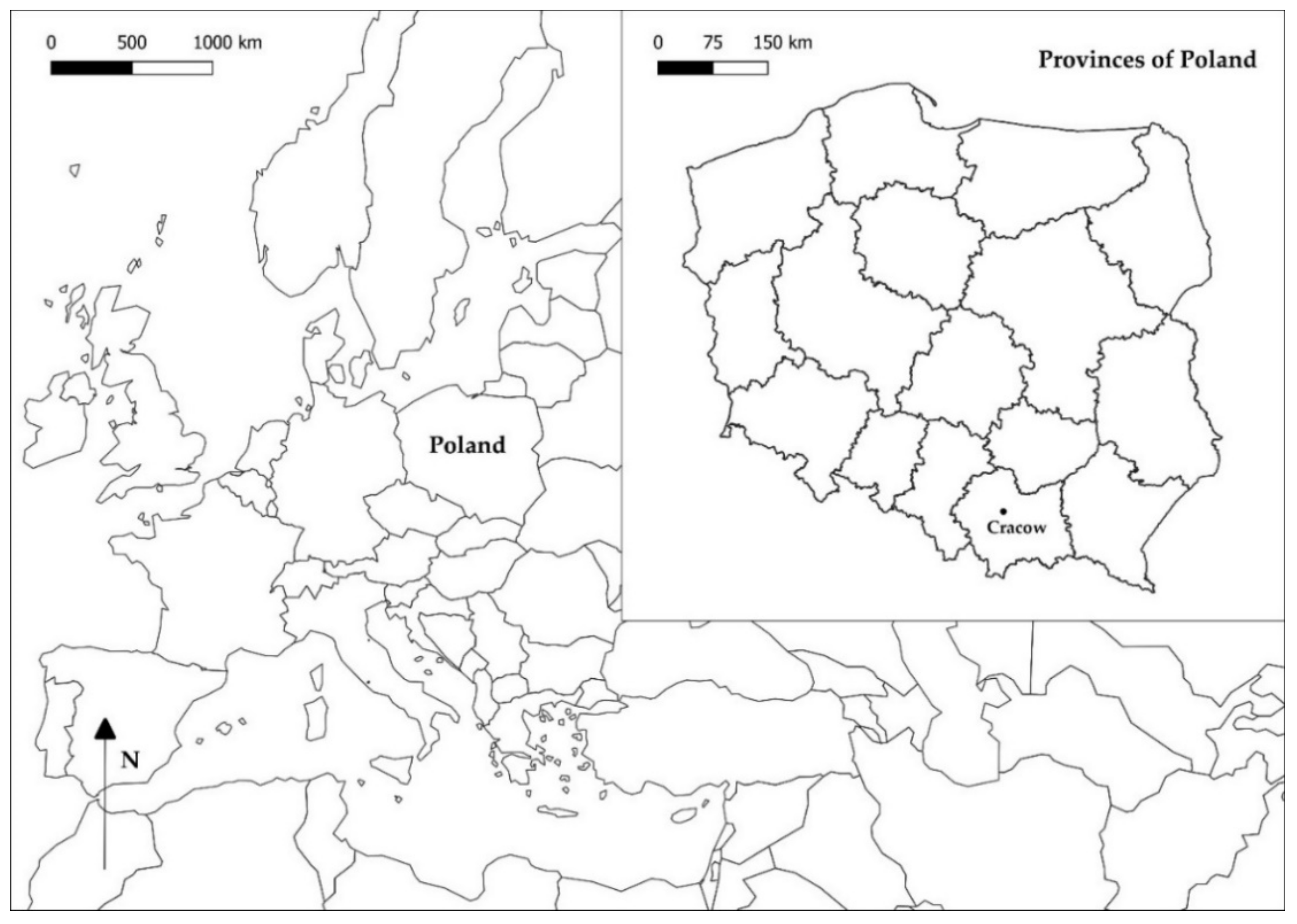
3.1. Study Area
3.2. Data Collection and Processing
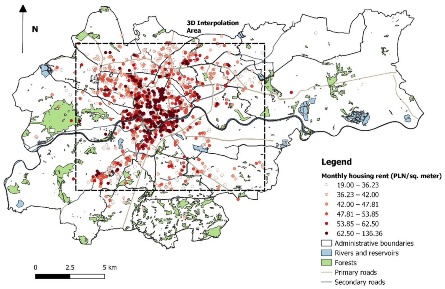
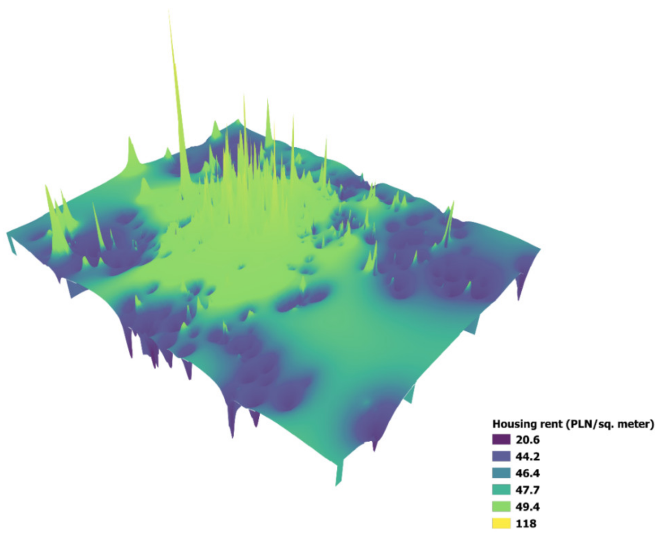
3.3. Spatial Distribution of Housing Rents
3.4. Independent Variables
3.5. Econometrics Models
4. Results and Discussion
4.1. OLS and SAR Model Estimates
4.2. GWR-SAR Model Estimates
4.3. Comparison of the Models
5. Conclusions
Supplementary Materials
Funding
Acknowledgments
Conflicts of Interest
Appendix A

| Number of Nearest Neighbours | AIC: SAR | AICc: SAR | AIC: GWR-SAR | AICc: GWR-SAR |
|---|---|---|---|---|
| 6 | 18,417.57 | 18,419.98 | 17,514.89 | 17,733.49 |
| 8 | 18,397.45 | 18,399.85 | 17,514.13 | 17,732.02 |
| 10 * | 18,373.00 | 18,375.40 | 17,508.26 | 17,725.91 |
| 12 | 18,377.28 | 18,379.68 | 17,522.07 | 17,739.70 |
| 14 | 18,374.65 | 18,377.05 | 17,527.10 | 17,743.97 |
| Variable | Mean | SD | Min | Median | Max | Percentage of Significant Cases at 95% | Percentage of Cases with Local VIF > 10 |
|---|---|---|---|---|---|---|---|
| Intercept | 61.630 | 33.836 | ‒201.480 | 59.322 | 148.515 | 45.74% | – |
| Structural variables | |||||||
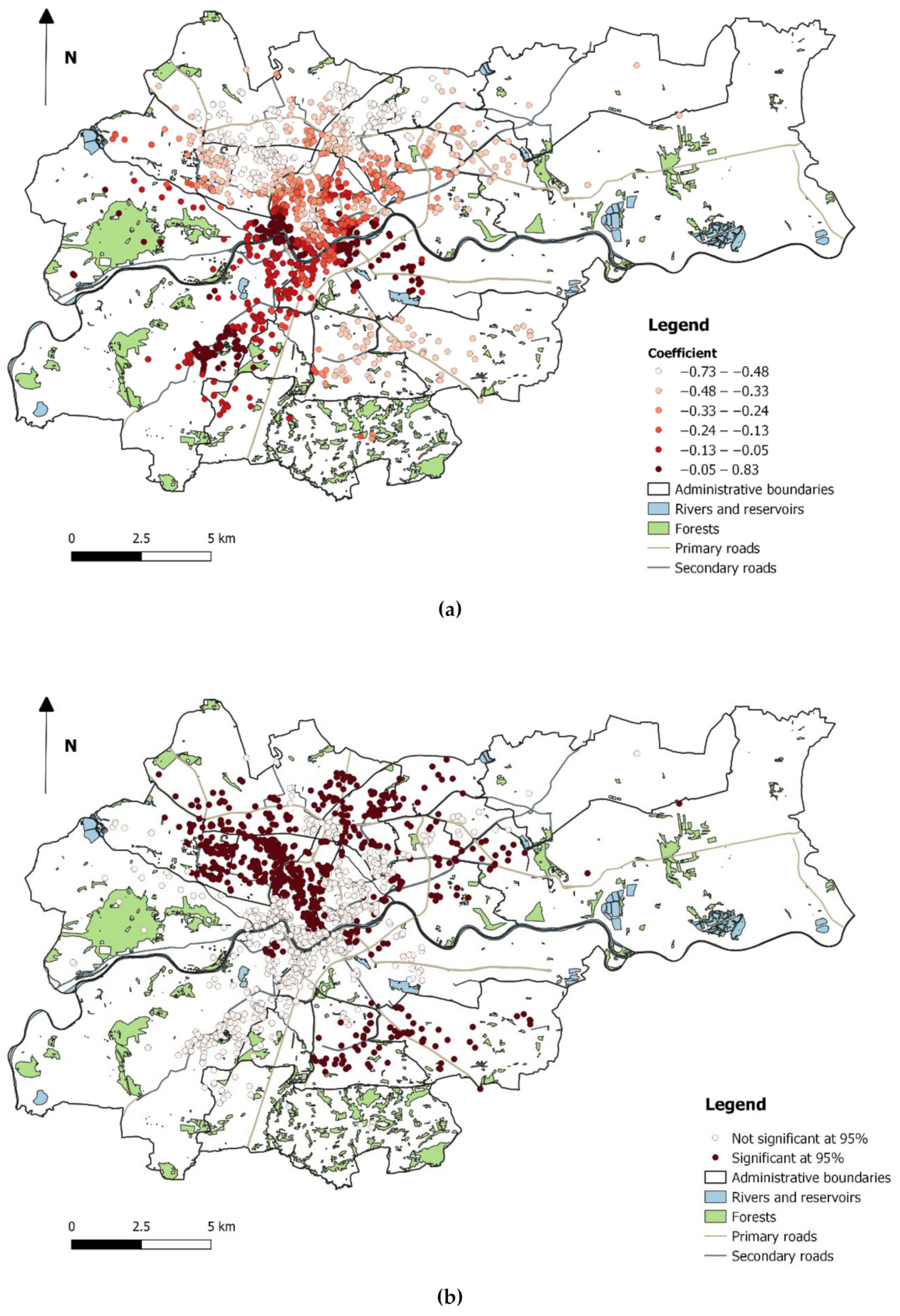
| FA | ‒0.240 | 0.223 | ‒0.734 | ‒0.233 | 0.809 | 51.26% | 0.00% |
| NR | 1.817 | 3.921 | ‒13.834 | 2.055 | 17.290 | 9.77% | 0.00% |
| FL | 0.314 | 0.772 | ‒3.098 | 0.109 | 3.243 | 8.23% | 0.00% |
| AA | 0.395 | 2.254 | ‒7.572 | 0.324 | 4.855 | 0.00% | 0.00% |
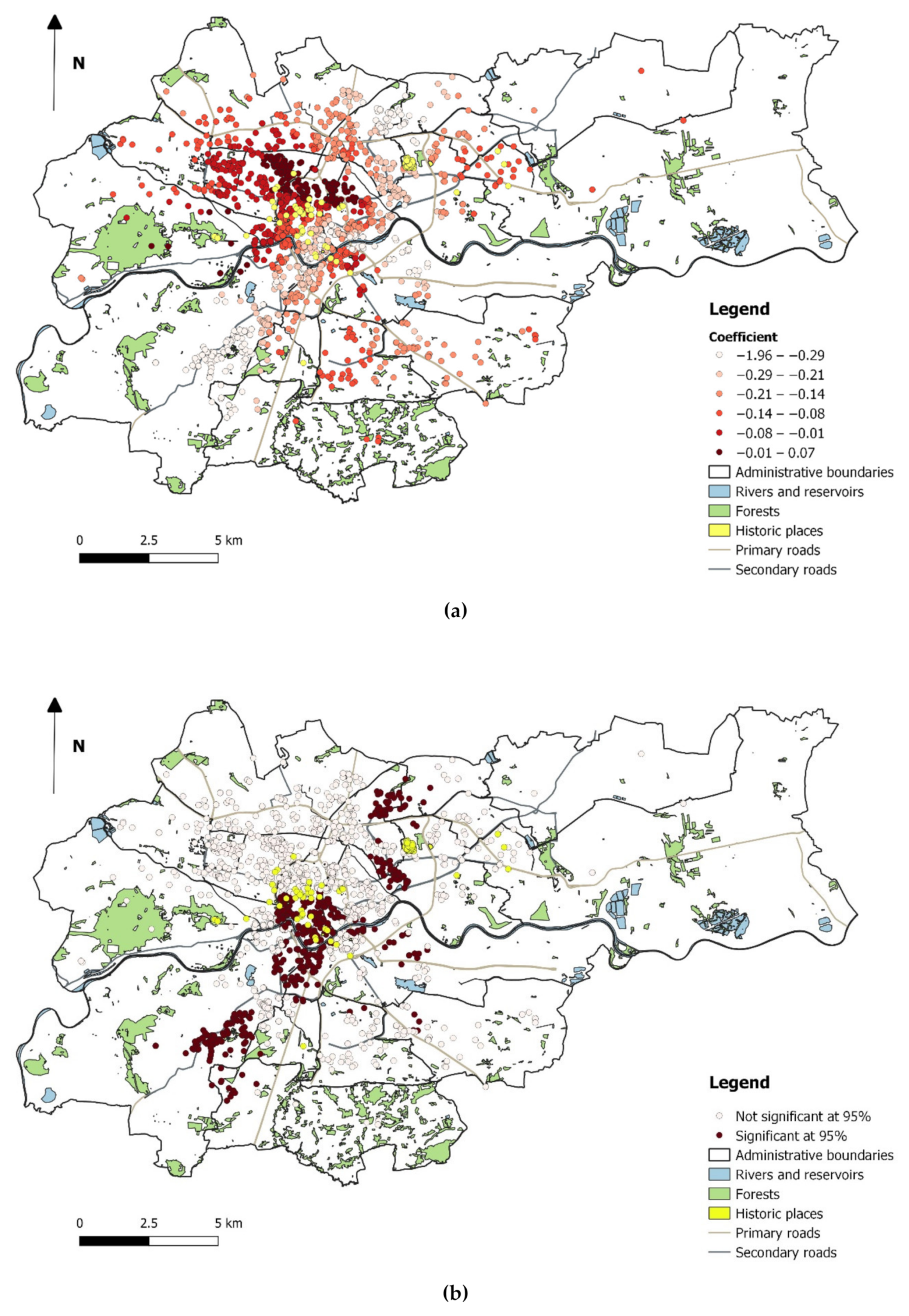
| AB | ‒0.163 | 0.174 | ‒1.960 | ‒0.143 | 0.070 | 34.42% | 0.00% |
| NF | ‒0.094 | 1.344 | ‒3.457 | ‒0.283 | 5.251 | 3.81% | 0.00% |
| AL | 3.185 | 5.101 | ‒15.527 | 2.672 | 16.069 | 14.27% | 0.00% |
| Locational variables | |||||||
| DPT | ‒0.008 | 0.025 | ‒0.086 | ‒0.006 | 0.088 | 10.03% | 6.47% |
| DR | 0.001 | 0.016 | ‒0.082 | 0.000 | 0.071 | 5.44% | 10.89% |
| Neighbourhood variables | |||||||
| DG | 0.004 | 0.023 | ‒0.054 | 0.000 | 0.186 | 5.62% | 17.45% |
| DW | ‒0.246 | 2.637 | ‒8.929 | ‒0.091 | 8.595 | 6.26% | 1.20% |
| DS | ‒0.003 | 0.017 | ‒0.063 | ‒0.001 | 0.089 | 9.34% | 12.26% |
| DU | ‒0.005 | 0.029 | ‒0.067 | ‒0.004 | 0.266 | 12.82% | 18.22% |
| DP | 0.473 | 2.739 | ‒10.937 | 0.322 | 9.507 | 5.53% | 3.17% |
| DSM | 0.003 | 0.014 | ‒0.069 | 0.000 | 0.063 | 8.92% | 20.27% |
| DSU | 1.087 | 3.251 | ‒6.698 | 0.564 | 30.373 | 7.76% | 5.57% |
| DPA | ‒0.662 | 3.843 | ‒18.275 | 0.216 | 9.206 | 5.53% | 7.63% |
| DRR | ‒0.008 | 0.023 | ‒0.19 | ‒0.002 | 0.022 | 6.56% | 25.72% |
References
- Hu, L.; He, S.; Han, Z.; Xiao, H.; Su, S.; Weng, M.; Cai, Z. Monitoring housing rental prices based on social media: An integrated approach of machine-learning algorithms and hedonic modeling to inform equitable housing policies. Land Use Policy 2019, 82, 657–673. [Google Scholar] [CrossRef]
- Tomal, M. Moving towards a Smarter Housing Market: The Example of Poland. Sustainability 2020, 12, 683. [Google Scholar] [CrossRef]
- Maalsen, S. Smart housing: The political and market responses of the intersections between housing, new sharing economies and smart cities. Cities 2019, 84, 1–7. [Google Scholar] [CrossRef]
- Gilbert, A. Rental housing: The international experience. Habitat Int. 2016, 54, 173–181. [Google Scholar] [CrossRef]
- Rubaszek, M.; Rubio, M. Does the rental housing market stabilize the economy? A micro and macro perspective. Empir. Econ. 2019. [Google Scholar] [CrossRef]
- Czerniak, A.; Rubaszek, M. The Size of the Rental Market and Housing Market Fluctuations. Open Econ. Rev. 2018, 29, 261–281. [Google Scholar] [CrossRef]
- Tomal, M. The Impact of Macro Factors on Apartment Prices in Polish Counties: A Two-Stage Quantile Spatial Regression Approach. Real Estate Manag. Valuat. 2019, 27, 1–14. [Google Scholar] [CrossRef]
- Tomal, M. House Price Convergence on the Primary and Secondary Markets: Evidence from Polish Provincial Capitals. Real Estate Manag. Valuat. 2019, 27, 62–73. [Google Scholar] [CrossRef]
- Geng, J.; Cao, K.; Yu, L.; Tang, Y. Geographically Weighted Regression model (GWR) based spatial analysis of house price in Shenzhen. In Proceedings of the 19th International Conference on Geoinformatics; IEEE: Shanghai, China, 2011; pp. 1–5. [Google Scholar]
- Liang, X.; Liu, Y.; Qiu, T.; Jing, Y.; Fang, F. The effects of locational factors on the housing prices of residential communities: The case of Ningbo, China. Habitat Int. 2018, 81, 1–11. [Google Scholar] [CrossRef]
- Liu, J.; Yang, Y.; Xu, S.; Zhao, Y.; Wang, Y.; Zhang, F. A Geographically Temporal Weighted Regression Approach with Travel Distance for House Price Estimation. Entropy 2016, 18, 303. [Google Scholar] [CrossRef]
- Mou, Y.; He, Q.; Zhou, B. Detecting the Spatially Non-Stationary Relationships between Housing Price and Its Determinants in China: Guide for Housing Market Sustainability. Sustainability 2017, 9, 1826. [Google Scholar] [CrossRef]
- Wu, C.; Ren, F.; Hu, W.; Du, Q. Multiscale geographically and temporally weighted regression: Exploring the spatiotemporal determinants of housing prices. Int. J. Geogr. Inf. Sci. 2019, 33, 489–511. [Google Scholar] [CrossRef]
- Zou, Y. Air Pollution and Housing Prices across Chinese Cities. J. Urban Plann. Dev. 2019, 145, 04019012. [Google Scholar] [CrossRef]
- Wu, B.; Li, R.; Huang, B. A geographically and temporally weighted autoregressive model with application to housing prices. Int. J. Geogr. Inf. Sci. 2014, 28, 1186–1204. [Google Scholar] [CrossRef]
- Cohen, J.P.; Coughlin, C.C.; Zabel, J. Time-Geographically Weighted Regressions and Residential Property Value Assessment. J. Real Estate Finan. Econ. 2020, 60, 134–154. [Google Scholar] [CrossRef]
- Geniaux, G.; Martinetti, D. A new method for dealing simultaneously with spatial autocorrelation and spatial heterogeneity in regression models. Reg. Sci. Urban Econ. 2018, 72, 74–85. [Google Scholar] [CrossRef]
- Li, D.-K.; Mei, C.-L.; Wang, N. Tests for spatial dependence and heterogeneity in spatially autoregressive varying coefficient models with application to Boston house price analysis. Reg. Sci. Urban Econ. 2019, 79, 103470. [Google Scholar] [CrossRef]
- Ma, Y.; Gopal, S. Geographically Weighted Regression Models in Estimating Median Home Prices in Towns of Massachusetts Based on an Urban Sustainability Framework. Sustainability 2018, 10, 1026. [Google Scholar] [CrossRef]
- Fotheringham, A.S.; Crespo, R.; Yao, J. Exploring, modelling and predicting spatiotemporal variations in house prices. Ann. Reg. Sci. 2015, 54, 417–436. [Google Scholar] [CrossRef]
- Yao, J.; Stewart Fotheringham, A. Local Spatiotemporal Modeling of House Prices: A Mixed Model Approach. Prof. Geogr. 2016, 68, 189–201. [Google Scholar] [CrossRef]
- Lu, B.; Charlton, M.; Harris, P.; Fotheringham, A.S. Geographically weighted regression with a non-Euclidean distance metric: A case study using hedonic house price data. Int. J. Geogr. Inf. Sci. 2014, 28, 660–681. [Google Scholar] [CrossRef]
- McCord, M.; Lo, D.; Davis, P.T.; Hemphill, L.; McCord, J.; Haran, M. A spatial analysis of EPCs in The Belfast Metropolitan Area housing market. J. Prop. Res. 2020, 37, 25–61. [Google Scholar] [CrossRef]
- McCord, M.J.; McCord, J.; Davis, P.T.; Haran, M.; Bidanset, P. House price estimation using an eigenvector spatial filtering approach. Intern. J. Hous. Mark. Anal. 2019. [Google Scholar] [CrossRef]
- McCord, M.J.; MacIntyre, S.; Bidanset, P.; Lo, D.; Davis, P. Examining the spatial relationship between environmental health factors and house prices: NO2 problem? J. Eur. Real Estate Res. 2018, 11, 353–398. [Google Scholar] [CrossRef]
- Huang, B.; Wu, B.; Barry, M. Geographically and temporally weighted regression for modeling spatio-temporal variation in house prices. Int. J. Geogr. Inf. Sci. 2010, 24, 383–401. [Google Scholar] [CrossRef]
- Dziauddin, M.F.; Ismail, K.; Othman, Z. Analysing the local geography of the relationship between residential property prices and its determinants. Bull. Geography. Socio-Econ. Ser. 2015, 28, 21–35. [Google Scholar] [CrossRef]
- Stewart Fotheringham, A.; Park, B. Localized Spatiotemporal Effects in the Determinants of Property Prices: A Case Study of Seoul. Appl. Spat. Anal. 2018, 11, 581–598. [Google Scholar] [CrossRef]
- Helbich, M.; Brunauer, W.; Vaz, E.; Nijkamp, P. Spatial Heterogeneity in Hedonic House Price Models: The Case of Austria. Urban Stud. 2014, 51, 390–411. [Google Scholar] [CrossRef]
- Helbich, M.; Griffith, D.A. Spatially varying coefficient models in real estate: Eigenvector spatial filtering and alternative approaches. Comput. Environ. Urban Syst. 2016, 57, 1–11. [Google Scholar] [CrossRef]
- Helbich, M.; Brunauer, W.; Hagenauer, J.; Leitner, M. Data-Driven Regionalization of Housing Markets. Ann. Assoc. Am. Geogr. 2013, 103, 871–889. [Google Scholar] [CrossRef]
- Osland, L.; Thorsen, I.S.; Thorsen, I. Accounting for local spatial heterogeneities in housing market studies. J. Reg. Sci. 2016, 56, 895–920. [Google Scholar] [CrossRef]
- Nordvik, V.; Osland, L.; Thorsen, I.; Thorsen, I.S. Capitalization of neighbourhood diversity and segregation. Environ. Plann. A 2019, 51, 1775–1799. [Google Scholar] [CrossRef]
- Cellmer, R.; Bełej, M.; Konowalczuk, J. Impact of a Vicinity of Airport on the Prices of Single-Family Houses with the Use of Geospatial Analysis. IJGI 2019, 8, 471. [Google Scholar] [CrossRef]
- Cellmer, R.; Trojanek, R. Towards Increasing Residential Market Transparency: Mapping Local Housing Prices and Dynamics. IJGI 2019, 9, 2. [Google Scholar] [CrossRef]
- Kobylińska, K.; Cellmer, R. Modelling and Simulation of Selected Real Estate Market Spatial Phenomena. IJGI 2019, 8, 446. [Google Scholar] [CrossRef]
- Olszewski, K.; Waszczuk, J.; Widłak, M. Spatial and Hedonic Analysis of House Price Dynamics in Warsaw, Poland. J. Urban Plann. Dev. 2017, 143, 04017009. [Google Scholar] [CrossRef]
- Trojanek, R.; Gluszak, M.; Tanas, J. The effect of urban green spaces on house prices in Warsaw. Int. J. Strateg. Prop. Manag. 2018, 22, 358–371. [Google Scholar] [CrossRef]
- Trojanek, R.; Gluszak, M. Spatial and time effect of subway on property prices. J. House Built Environ. 2018, 33, 359–384. [Google Scholar] [CrossRef]
- Li, H.; Wei, Y.D.; Wu, Y. Analyzing the private rental housing market in Shanghai with open data. Land Use Policy 2019, 85, 271–284. [Google Scholar] [CrossRef]
- Zhang, S.; Wang, L.; Lu, F. Exploring Housing Rent by Mixed Geographically Weighted Regression: A Case Study in Nanjing. IJGI 2019, 8, 431. [Google Scholar] [CrossRef]
- Cui, N.; Gu, H.; Shen, T.; Feng, C. The Impact of Micro-Level Influencing Factors on Home Value: A Housing Price-Rent Comparison. Sustainability 2018, 10, 4343. [Google Scholar] [CrossRef]
- Leung, K.M.; Yiu, C.Y. Rent determinants of sub-divided units in Hong Kong. J. House Built Environ. 2019, 34, 133–151. [Google Scholar] [CrossRef]
- Efthymiou, D.; Antoniou, C. How do transport infrastructure and policies affect house prices and rents? Evidence from Athens, Greece. Transp. Res. Part A: Policy Pract. 2013, 52, 1–22. [Google Scholar] [CrossRef]
- Crespo, R.; Grêt-Regamey, A. Local Hedonic House-Price Modelling for Urban Planners: Advantages of Using Local Regression Techniques. Environ. Plan. B Plan. Des. 2013, 40, 664–682. [Google Scholar] [CrossRef]
- McCord, M.; Davis, P.T.; Haran, M.; McIlhatton, D.; McCord, J. Understanding rental prices in the UK: A comparative application of spatial modelling approaches. Int. J. House Mark. Anal. 2014, 7, 98–128. [Google Scholar] [CrossRef]
- Suárez-Vega, R.; Hernández, J.M. Selecting Prices Determinants and Including Spatial Effects in Peer-to-Peer Accommodation. IJGI 2020, 9, 259. [Google Scholar] [CrossRef]
- Santana-Jiménez, Y.; Suárez-Vega, R.; Hernández, J.M. Spatial and environmental characteristics of rural tourism lodging units. Anatolia 2011, 22, 89–101. [Google Scholar] [CrossRef]
- Santana-Jiménez, Y.; Sun, Y.-Y.; Hernández, J.M.; Suárez-Vega, R. The Influence of Remoteness and Isolation in the Rural Accommodation Rental Price among Eastern and Western Destinations. J. Travel Res. 2015, 54, 380–395. [Google Scholar] [CrossRef]
- Hanink, D.M.; Cromley, R.G.; Ebenstein, A.Y. Spatial Variation in the Determinants of House Prices and Apartment Rents in China. J. Real Estate Finan. Econ. 2012, 45, 347–363. [Google Scholar] [CrossRef]
- Nalepka, A.; Tomal, M. Identyfikacja czynników kształtujących ceny ofertowe deweloperskich lokali mieszkalnych na obszarze jednostki ewidencyjnej Nowa Huta. Świat Nieruchom. (World Real Estate J.) 2016, 11–18. [Google Scholar] [CrossRef]
- Brzezicka, J.; Łaszek, J.; Olszewski, K.; Waszczuk, J. Analysis of the filtering process and the ripple effect on the primary and secondary housing market in Warsaw, Poland. Land Use Policy 2019, 88, 104098. [Google Scholar] [CrossRef]
- Gluszak, M.; Marona, B. Discrete choice model of residential location in Krakow. J. Eur. Real Est. Res. 2017, 10, 4–16. [Google Scholar] [CrossRef]
- National Bank of Poland. Sytuacja na Lokalnych Rynkach Nieruchomości Mieszkaniowych w Polsce w 2018. National Bank of Poland: Warsaw, Poland, 2019. [Google Scholar]
- Yang, W. An Extension of Geographically Weighted Regression with Flexible Bandwidths. Ph.D. Thesis, University of St Andrews, St Andrew, UK, 2015. [Google Scholar]
- Tomal, M.; Nalepka, A. The impact of social participation on the efficiency of communal investment expenditure. Econ. Res. Ekon. Istraživanja 2020, 33, 477–500. [Google Scholar] [CrossRef]
- Basile, R.; Durbán, M.; Mínguez, R.; María Montero, J.; Mur, J. Modeling regional economic dynamics: Spatial dependence, spatial heterogeneity and nonlinearities. J. Econ. Dyn. Control 2014, 48, 229–245. [Google Scholar] [CrossRef]
- Dubé, J.; Legros, D.; Thériault, M.; Des Rosiers, F. Measuring and Interpreting Urban Externalities in Real-Estate Data: A Spatio-Temporal Difference-in-Differences (STDID) Estimator. Buildings 2017, 7, 51. [Google Scholar] [CrossRef]
- Anselin, L. Spatial Econometrics. In A Companion to Theoretical Econometrics; Baltagi, B.H., Ed.; Blackwell Publishing Ltd.: Malden, MA, USA, 2003; pp. 310–330. [Google Scholar]
- da Silva, A.R.; Fotheringham, A.S. The Multiple Testing Issue in Geographically Weighted Regression: The Multiple Testing Issue in GWR. Geogr. Anal. 2016, 48, 233–247. [Google Scholar] [CrossRef]
- Małkowska, A.; Palus, E. Wpływ sąsiedztwa rzeki Wisły na poziom cen ofertowych nowych lokali mieszkalnych w Krakowie. World Real Estate J. (Swiat Nieruchom.) 2017, 101, 63–68. [Google Scholar]
- Adamkiewicz, D.; Radziszewska-Zielina, E. A housing market analysis for the city of Krakow. Czas. Tech. 2019, 2019, 57–70. [Google Scholar] [CrossRef]
- Głuszak, M. Externalities and House Prices: A Stated Preferences Approach. EBER 2018, 6, 181–196. [Google Scholar] [CrossRef]


| Group | Category | Definition | Form | Abbrev. |
|---|---|---|---|---|
| Structure | Flat | Floor area (m2) | Standard | FA |
| Number of rooms | Standard | NR | ||
| Floor level | Standard | FL | ||
| Availability of additional space (garage, usable room, basement) | Standard | AA | ||
| Building | Age of the building in years | Standard | AB | |
| Number of floors in the building | Standard | NF | ||
| Availability of lift in the building | Standard | AL | ||
| Type of building (block, tenement, apartment, house)—four dummy variables | Variables deleted because of high variance inflation factor (VIF) values | – | ||
| Location | Public transport | Distance to nearest bus stop, tram stop or train stop (m) | Standard | DPT |
| Road accessibility | Distance to nearest primary or secondary road (m) | Standard | DR | |
| City centre | Distance to city centre (m) | Variable deleted because of high VIF value | – | |
| Neighbour-hood | Publicfacilities | Distance to nearest local government building (m) | Standard | DG |
| Job opportunities | Distance to nearest workcentre (m) | Logarithmic | DW | |
| Education facilities | Distance to nearest school (m) | Standard | DS | |
| Distance to nearest university (m) | Standard | DU | ||
| Healthcare facilities | Distance to nearest pharmacy (m) | Logarithmic | DP | |
| Commercial facilities | Distance to nearest shoppingmall (m) | Standard | DSM | |
| Distance to nearestsupermarket (m) | Logarithmic | DSU | ||
| Natural amenities | Distance to nearest park (m) | Logarithmic | DPA | |
| Distance to nearest river or reservoir (m) | Standard | DRR |
| Variable | OLS | SAR |
|---|---|---|
| Intercept | 59.261 *** | 25.656 *** |
| Structural variables | ||
| FA | ‒0.059*** | ‒0.072*** |
| NR | ‒0.803 | ‒0.462 |
| FL | 0.135 | 0.352 ** |
| AA | ‒0.621 | ‒0.410 |
| AB | ‒0.067 *** | ‒0.061 *** |
| NF | ‒0.691 *** | ‒0.483 *** |
| AL | 8.165 *** | 4.870 *** |
| Locational variables | ||
| DPT | ‒0.011 *** | ‒0.002 |
| DR | 0.001 | 0.000 |
| Neighbourhood variables | ||
| DG | ‒0.001 *** | ‒0.000 |
| DW | 0.103 | ‒0.159 |
| DS | ‒0.005 *** | ‒0.002 * |
| DU | ‒0.004 *** | ‒0.001 *** |
| DP | 0.604 | 0.444 |
| DSM | ‒0.000 | 0.001 |
| DSU | 1.380 *** | 0.173 |
| DPA | ‒1.171 *** | ‒0.984 *** |
| DRR | ‒0.003 *** | ‒0.001 * |
| Wy | NA | 0.665 *** |
| 2336 | 2336 | |
| 18,518.60 | 18,373.00 | |
| 18,520.96 | 18,375.40 | |
| 0.24 | 0.28 | |
| Variable | Mean | SD | Min | Median | Max | Percent of Significant Cases at 95% | Percent of Cases with Local VIF > 10 | MC |
|---|---|---|---|---|---|---|---|---|
| Intercept | 51.486 | 49.589 | −195.165 | 46.798 | 283.054 | 10.74% | − | SN |
| Structural variables | ||||||||
| FA | −0.243 | 0.222 | −0.734 | −0.239 | 0.825 | 52.40% | 0.00% | SN |
| NR | 1.862 | 3.879 | −14.150 | 2.045 | 17.324 | 9.85% | 0.00% | SN |
| FL | 0.331 | 0.746 | −3.126 | 0.142 | 3.111 | 7.58% | 0.00% | SN |
| AA | 0.428 | 2.210 | −8.033 | 0.372 | 4.893 | 0.21% | 0.00% | SN |
| AB | −0.166 | 0.174 | −1.955 | −0.144 | 0.068 | 35.40% | 0.00% | SN |
| NF | −0.113 | 1.303 | −3.356 | −0.262 | 4.608 | 4.79% | 0.09% | SN |
| AL | 2.978 | 5.087 | −15.567 | 2.382 | 15.395 | 14.04% | 0.00% | SN |
| Locational variables | ||||||||
| DPT | −0.005 | 0.028 | −0.089 | −0.002 | 0.102 | 8.82% | 6.77% | SN |
| DR | 0.001 | 0.018 | −0.103 | −0.001 | 0.082 | 6.46% | 13.16% | SN |
| Neighbourhood variables | ||||||||
| DG | 0.007 | 0.022 | −0.043 | 0.002 | 0.183 | 6.55% | 22.03% | SN |
| DW | −0.561 | 2.623 | −9.426 | −0.422 | 8.061 | 5.31% | 1.20% | SN |
| DS | −0.001 | 0.017 | −0.061 | 0.000 | 0.119 | 7.15% | 12.69% | SN |
| DU | −0.003 | 0.028 | −0.057 | −0.003 | 0.260 | 6.46% | 21.30% | SN |
| DP | 0.330 | 2.741 | −9.234 | 0.128 | 9.819 | 2.95% | 3.90% | SN |
| DSM | 0.002 | 0.015 | −0.081 | 0.001 | 0.064 | 7.41% | 22.29% | SN |
| DSU | 0.826 | 3.215 | −7.531 | 0.278 | 40.072 | 4.45% | 5.57% | SN |
| DPA | −0.658 | 3.922 | −19.560 | 0.264 | 11.465 | 5.39% | 8.02% | SN |
| DRR | −0.007 | 0.023 | −0.187 | −0.001 | 0.036 | 4.49% | 26.53% | SN |
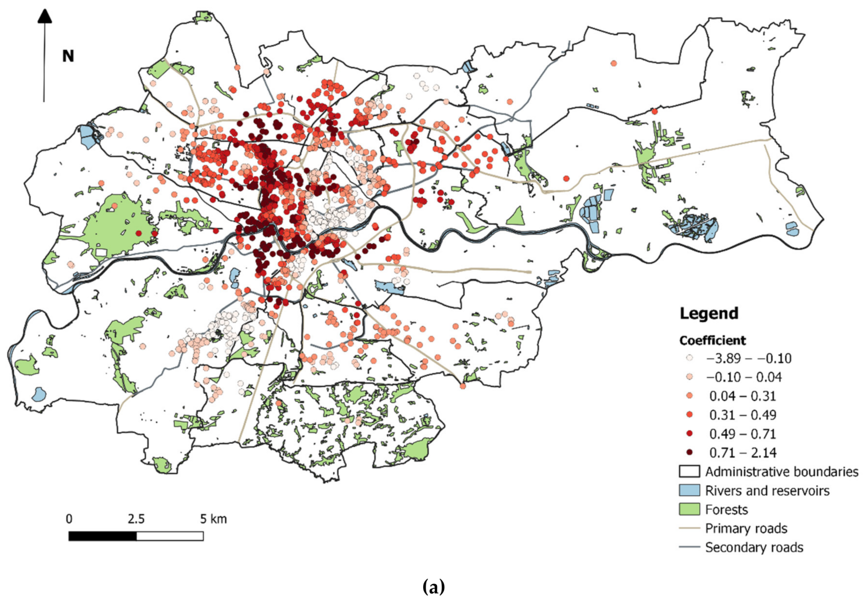
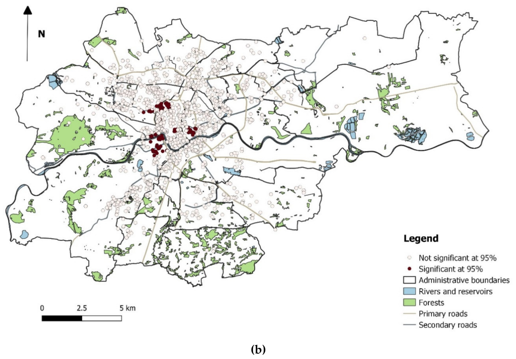
| Wy | 0.205 | 0.713 | −3.893 | 0.308 | 2.140 | 6.85% | 6.34% | SN |
| 2,336 | ||||||||
| 17,508.26 | ||||||||
| 17,725.91 | ||||||||
| 0.66 | ||||||||
| Model | AIC | RMSE | |
| OLS | 18,518.60 | 12.70 | 0.24 |
| SAR | 18,373.00 | 12.31 | 0.28 |
| GWR * | 17,520.78 | 8.59 | 0.65 |
| GWR-SAR | 17,508.26 | 8.50 | 0.66 |
© 2020 by the author. Licensee MDPI, Basel, Switzerland. This article is an open access article distributed under the terms and conditions of the Creative Commons Attribution (CC BY) license (http://creativecommons.org/licenses/by/4.0/).
Share and Cite
Tomal, M. Modelling Housing Rents Using Spatial Autoregressive Geographically Weighted Regression: A Case Study in Cracow, Poland. ISPRS Int. J. Geo-Inf. 2020, 9, 346. https://doi.org/10.3390/ijgi9060346
Tomal M. Modelling Housing Rents Using Spatial Autoregressive Geographically Weighted Regression: A Case Study in Cracow, Poland. ISPRS International Journal of Geo-Information. 2020; 9(6):346. https://doi.org/10.3390/ijgi9060346
Chicago/Turabian StyleTomal, Mateusz. 2020. "Modelling Housing Rents Using Spatial Autoregressive Geographically Weighted Regression: A Case Study in Cracow, Poland" ISPRS International Journal of Geo-Information 9, no. 6: 346. https://doi.org/10.3390/ijgi9060346
APA StyleTomal, M. (2020). Modelling Housing Rents Using Spatial Autoregressive Geographically Weighted Regression: A Case Study in Cracow, Poland. ISPRS International Journal of Geo-Information, 9(6), 346. https://doi.org/10.3390/ijgi9060346