Visualizing the USA’s Maritime Freight Flows Using DM, LP, and AON in GIS

Abstract

In this research, we developed a novel model framework consisting of data mining (DM), linear programming (LP), and an all-or-nothing (AON) flow assignment to estimate maritime freight flows between the United States and the rest of the world. We first built DM and LP models to select and combine various country-level data sources on import and export freight into a complete geographic information system (GIS)-based origin and destination (OD) database with targeted locations, networks, and attributes on ocean routes connecting foreign and U.S. maritime ports. Then, we performed freight assignments and estimated total or commodity-specific import and export freight flows. Additionally, we visualized major sea ports with various handling capacities and optimal maritime freight flows in 2D in GIS and in 3D in Google Earth with highlights for selected total and most imported or exported goods on maritime networks and for major trading partners, such as the U.S. and China. Finally, a visual validation of model results on optimal maritime routes with respect to real-time vessel density network links and routes was provided as well.

1. Introduction

International trade of goods is largely realized through import and export of commodities shipped by maritime vessels on global networks consisting of sea ports and ocean routes. International trade of goods, also regarded as global freight flow to and from a country, is critical to the country’s economy. For example, the total international trade value in goods in 2018 for the United States was $4.236 trillion, including $1.674 trillion for exports, $2.562 trillion for imports, and $0.888 trillion for trade deficits, representing about 20.66% of the gross domestic products in the U.S. [1]. The total national economic impact of the maritime system, including maritime ports and shipping, was about $5.40 trillion in value, 30.78 million in employment, and $378.10 billion in taxes [2]. The maritime freight shipping sector recorded $164 billion in revenue, of which 80.9% was realized by containerized freight. The sector is going to grow to $210 billion by 2021 [3]. Selected scholarly research on benefits of freight trade the economy at various levels can be found in Nordas et al. [4] 2006, Djankov et al. [5], and Gani [6].

The majority of global imports and exports is realized by maritime cargo containers for manufactured goods and/or intermediate parts. For example, of the goods to and from the U.S. by maritime means in 2018, 59% arrived at and 61% shipped from the country by containers on vessels. In twenty-foot equivalent units (TEU), the top five U.S. import and export sea ports included Los Angeles, Long Beach, New York/New Jersey, Savannah, and Northwest Seaport Alliance. Similarly, the top world sea ports in terms of TEU were Shanghai, Singapore, Shenzhen, Ningbo-Zhoushan, and Guangzhou. The top five trading partners by value for the United States were China, Canada, Mexico, Japan, and Germany. The top five U.S. exported or imported goods were industrial machinery, oil and mineral fuels, electrical machinery, aircraft, moto vehicles and parts, and pharmaceuticals [1,7].

In this study, we aimed to estimate and visualize U.S. import and export shipments or freight flows on global maritime networks as proxies for U.S. international trade of goods during 2008–2018. This paper is structured as follows: Section 2 provides a concise review of relevant literature. Section 3 describes the necessary databases and their integration issues for U.S. maritime import–export freight and networks. Section 4 develops the integrated model framework, which contains DM (Data Mining), LP (Linear Programming), and AON (All or Nothing) sub-models and software integration issues. Section 5 presents key results and visualization of global freight flows between the U.S. and the world, including the largest ports in terms of handling goods by weight, value, and TEU; optimal flows on routes; and total or specific commodities in 2D or 3D graphics. A visual comparison of modeled optimal routes against real-time vessel density routes was conducted as a way of validating the model framework and its results.

Previous modeling studies on global maritime freight, reviewed below, are mostly based upon push and pull using gravity-type spatial interaction models, statistical econometric methods, logistics or supply chains approaches, and real time maritime vessel tracking using global positioning systems. The major contribution of this study relies on its optimization framework, which integrates freight data through data mining, performs a freight assignment, and visualizes maritime routes and volumes. In addition, the scape of this study in terms of countries (220 +), sea ports (4000 +), maritime port-port networks (tens of thousands of links and routes) covering the world oceans, goods (different kinds in tens of thousands), and measurement units (value, weight, and TEU) is large and diverse and not seen in the existing literature.

2. Related Work

Goods for maritime trade are largely carried on vessels between the sea ports of two countries. These sea ports and the connecting ocean routes form the global maritime trade network. Goods flows in the network are often called ocean freight, which is commonly measured in value (e.g., dollars), by weight (e.g., tons), or by container (e.g., TEU), and classified by a scheme (e.g., harmonized system). Ocean containers are the dominant form of maritime freight; others include flatrack, platform, bulk, tanks, etc.

The international trade and maritime freight literature is vast, including Lowe [8] on technical and policy issues of intermodal freight and Liu and Xin [9], who constructed a numerical model to demonstrate the impact of the shipment time uncertainty of imported goods and transportation improvements on international trade growth. Yip [10] introduced a gravity model of trade to study economic factors, such as population, GDP, and development level, on the international import and export grain freight flows between major trading countries over the period of 1996–2006.

Ocean freight flows and networks were studied by Hayuth and Fleming [11] with centrality and accessibility of strategic container sea ports as gateways and transit points for international trade from the perspectives of carriers and shippers and their dynamics and relevance at variable geographical scales, transport development, and port sophistication. Montes et al. [12] completed a graph theoretical complex networks analysis of the current maritime network’s evolution based on throughput rise and fall at ports and on ocean routes for containerized and general cargo. Ducruet et al. [13] used graph and cluster measures of maritime freight movements to show that the hub-and-spoke strategies and networks for sea ports and maritime shipments in the Atlantic Ocean became dominant for more shipping liners.

Maritime freight port capacity issues, determined through a survey of ports for rising container volumes, requiring immediate solutions to worsening port congestion and coordination among stakeholders, including governments, labor unions, and carriers of various modes, were addressed by Maloni and Jackson [14]. U.S. sea port selection and carrier choice for efficient intermodal freight were investigated by Klodzinski and Haitham [15], who used an artificial neural network model to study, with estimation and validation, the freight accessibility, and to forecast freight volumes of truck transportation to sea port terminals at Port of Tampa and Port Canaveral in Florida. Malchow and Kanafani [16] used a discrete choice model to analyze maritime freight flows among U.S. sea ports through an assignment function of vessel shipment and port attributes, including commodity type, geographical location, and carrier.

Waters [17] and Notteboom and Rodrigue [18] studied port regionalization and port–hinterland system development calls for new port governance and function. Verhetsel and Sel [19] studied and classified world maritime cities as those with sea port terminal operators and local container business connections, plus national and international linkages. Deng et al. [20] used a structural equation model to study the relationship between a port regarding its supply, demand, and value-added activity and its regional economy. Wang [21] studied the impact of Ocean Shipping Reform Act (OSRA) through inbound and outbound trade freight volumes and rates for transatlantic trade routes and found that the OSRA forced carriers to become more competitive. Heaver [22] argued for port cost recovery, local autonomy, direct management responsibility, and inter-port collaboration for shared and better port services; Wang et al. [23] used a governance approach to study the recent institutional changes in China’s port industry along with China’s port management internalization.

The studies summarized above focused more on ocean freight networks, ports, and operations, which are important, but are indirectly related to maritime system-wide freight flows. When freight flows were considered directly, they were only local (i.e., a port, a shipper/carrier, or country) or regional (i.e., a continent or a trade organization) in scope. Shen [24,25] considered global trade flows with the U.S., but the integrated models in these studies were not mathematically specified because their focuses were on conceptualization and data processing. Additionally, no validation of the results was conducted. Global maritime system-wide freight flow studies are lacking.

Our research is novel in that we explored the U.S. imported and exported goods as global maritime freight flows through the entire maritime networks for the world. This is particularly important as the U.S. economy is the largest and trades with more than 220 countries. We therefore used the world maritime network to study the U.S.-world maritime trade flows. Here, we regard freight flows as the annual aggregated movement of vessels loaded with various goods by weight, value, or TEU, regardless specific shippers/carriers. The maritime network consists of imaginary ocean routes on which vessels move goods as imports and exports between ports of any two countries. Specifically, this research examines maritime freight movement on the maritime network for the period of 2008–2018 with a framework consisting of three optimization models, including data mining to find the most suitable attributes, data integration to form the target database, and flow assignment under the system optimality, by integrating publicly available databases and visualizing the U.S. freight flows in the global maritime network in 2D and 3D. We highlight the optimal flow patterns and routes of U.S. ocean freight as proxies to the U.S.’s international trade of goods. We also provid a visual approach to the validation of the optimal maritime time links and routes.

3. Databases

Many public and private databases are available regarding the U.S.’s maritime freight flows, including import and export, port, and network databases. However, these databases contain diverse attributes with variable utility and accuracy levels with respect to the targeted database and its desired attributes. Hence, data mining to screen all plausible source databases and then integrate the identified ones to get the targeted data are necessary steps for this study. The target database must have attributes describing freight flows, such as commodity types (e.g., by harmonized schedule), measurement units (e.g., by weight, value, or TEU), port attributes showing origin and destination (OD) information (e.g., port ID, country name, location by longitude and latitude), and network routes (e.g., route id, distances, capacities, and assigned flows).

3.1. Freight Databases

Table 1. Freight and port databases and attributes.

Data Source	OD Pair	Commodity Code	History	Frequency	Unit	Geographic Information	Cost
S1	U.S. metros	STCC, SCTG	1993, 1997, 2002, 2007	Yearly	Weight, Value	Detail to U.S. metropolitans area	Free
S2	Countries, States	HS, SITC, NAICS	1999–2018	Yearly	Value	None	Free
S3	U.S. ports, District, World regions	SCTG	2002–2045	Yearly	Weight, Value	U.S. ports, district, world regions	Free
S4	U.S. ports, Countries	None	1997–2018	Yearly	TEU, Weight	None	Free
S5	U.S. ports, Countries	HS	2003–Now	Monthly	Weight, Value	None	Limited Free
S6	U.S. ports, Countries	Harmonized tariff code, JOC	1992–2018	Daily	Weight, Value TEU, etc.	U.S. port, countries	Paid
S7	U.S. ports, International ports	PMS	1997–2018	Yearly	Weight	U.S ports, international ports	Free
S8	None	None	None	None	None	International waterways	Free
S9	None	None	None	None	None	U.S ports, international ports	Free

shows some freight data with attributes such as commodity codes; port IDs or names; units; OD matrices; and transportation modes, tons, and values. Here, S1 = commodity flow survey (CFS), S2 = TradeStats Express, S3 = Freight Analysis Freight or (FAF) with U.S. domestic networks, including waterways, S4 = Maritime Administration database (MARAD) in which Schedule K contains U.S. goods import and export information, S5 = US Trade Online, S6 = PIERS global intelligence Solutions, S7 = US Army Corps of Engineer Navigation Data Center (NDC), S8 = Oak Ridge National Laboratory (ORNL) Waterway Network, and World Port Index (WPI). S1–S9 were selected from initial 15 databases from pubic sources (free) and private sources (for a fee), each containing 15 to 20+ attributes. The final databases used for this study were all obtained from pubic sources.

The Maritime Administration Database (MARAD) provides maritime import and export freight flow by port, partner, tonnage, and container [26]. However, MARAD does not contain goods classifications and omits some port OD pairs. USA Trade Online [27] provides official U.S. import and export trade data between foreign countries and U.S. ports at a monthly frequency. This online database is based on the 6-digit North America Industry Classification System (NAICS) by the U.S. Census Bureau [1] and the 10-digit Harmonized System (HS) by the World Customs Organization [28]. The Navigation Data Center (NDC) provides yearly and port-level U.S. coastal and inland waterway database by U.S. Army Corps of Engineers [29]. The database contains information on countries, cargoes, facilities, waterways, terminals, etc., including 200 + U.S. ports, 1000 + foreign ports, and goods classified by the lock performance monitoring system (LPMS) or (PMS).

3.2. Port Databases

Since the global freight flow is mostly shipped between maritime ports, studying port-to-port freight movement is important to understand international trade. Here, the geographic information of maritime ports is critical. Two databases, NDC and World Port Index (WPI) by Landfall Navigation [30], contain the geographic locations and other attributes for major U.S. ports and foreign ports.

The geographical locations of U.S. and international ports are specified by their longitudes and latitudes. However, only a few of the 1813 foreign ports in the NDC database have their longitudes and latitudes, whereas the WPI database has 4043 maritime ports with longitudes and latitudes, including all U.S. ports; hence, we used WPI in this research.

3.3. Network Databases

The NDC database contains detailed U.S. coasts ports, routes, and inland waterways, but limited information on the global maritime network. FAF database contains networks mostly for U.S. highways. However, the global maritime network by Oak Ridge National Laboratory (ORNL) [31] is complete with existing ocean routes for both the United States and the world and a grid mash covering all oceans for possible new or more optimal maritime routes. The ORNL network also contains U.S. domestic highway, rail, and inland water networks, and intermodal points. 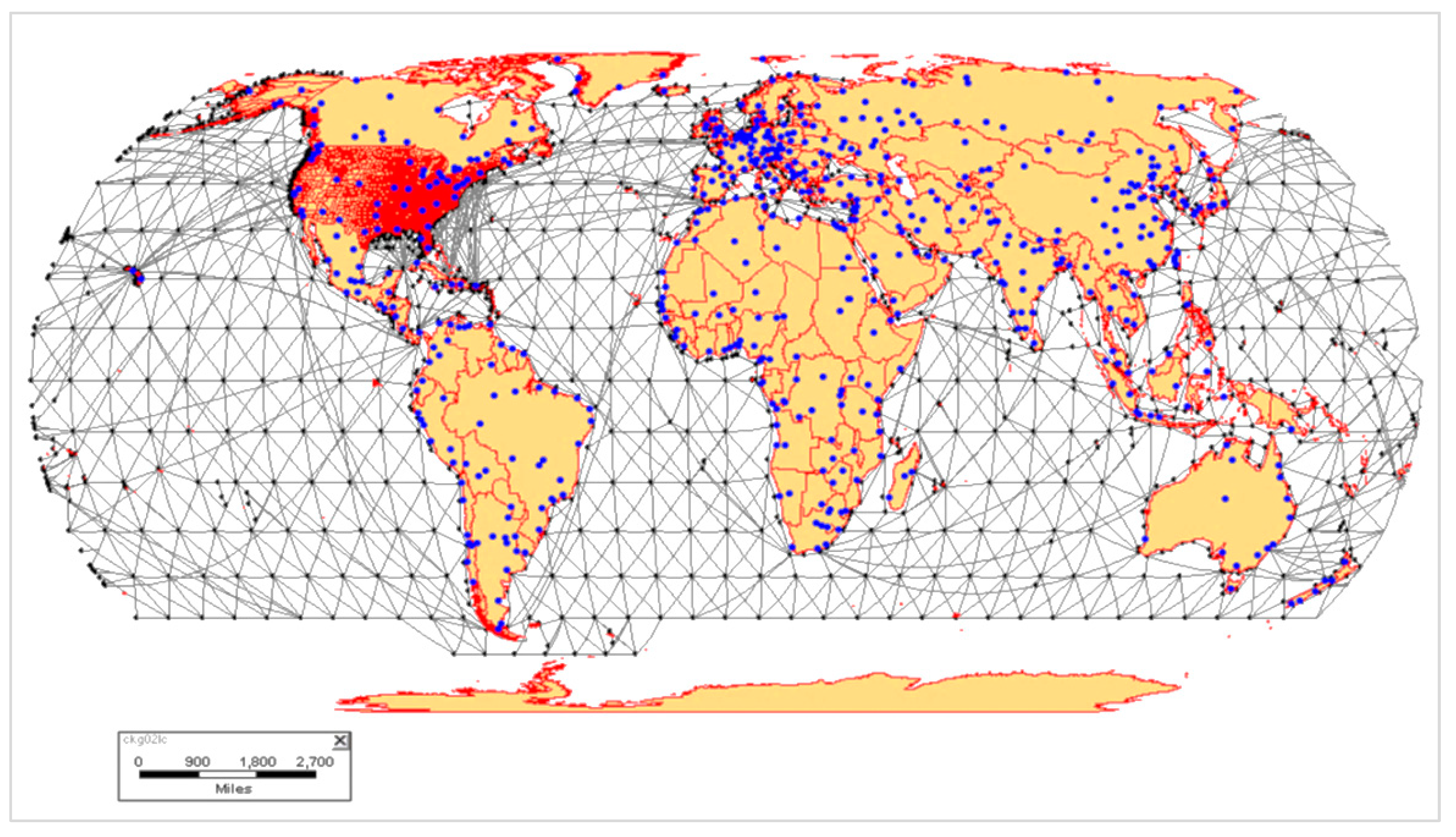Figure 1 depicts a complete global maritime network containing grid and actual routes (in grey), 4000 + ports (in blue), and 250 + countries (in orange). This network is the outcome of combined NDC and ORNL networks and can only be used for assignment after further combining with WPI for port locations and freight flow information, which is primarily from the Schedule K in MARAD. The combination also involved some GIS data cleaning and processes, such as network routes alignment and ports.

3.4. Code Match Issue in Databases

Having diverse codes and levels for the freight databases was a major issue encountered in this research. First, several types of commodity codes are produced by different agencies or governments; the Standard International Trade Classification (SITC) and the Harmonized Commodity Description and Coding Systems (HS) classify commodities at 2, 4, 6, 8 or 10-digital levels, making matching these codes a cumbersome task. Second, the corresponding industries primarily for the commodities are also classified in multiple ways by multiple codes, especially for early databases. For example, the older Standard Industry Classification (SIC) and the newer North American Industry Classification System (NAICS), each with up to six digits, are also hard to match with each other exactly. Third, matching industry and commodity codes is even harder when forecasts are needed for certain spatial units (i.e., state, country, or district) from historical data to the present or the future, for domestic (D) and foreign (F), for end-use or for specific industries, such as high technologies (e.g., Hi-tech) specified by country or agriculture or not (e.g., Ag/Non Ag) classified by the U.S. Department of Agriculture (USDA). In national input–output tables, three basic end-users are intermediate, household consumption, and capital goods [32]. These codes, with their spatial levels (i.e., port, state, and country) and classification digits are summarized in

Table 2. Common commodity and industry classifications and matching.

Data Code	Level of Detail for Exports	Level of Detail for Imports
HS	2–10 digits HS by country, by district, by DF	2–10 digits HS by country by district, by DF
HS by State	2–6 digits HS by country, by state	2–6 digits HS by country, by state
HS by Port	2–6 digits HS by country, by port	2–6 digits HS by country, by port
NAICS-1	2–6 digits NAICS by country, by district, by DF	2–6 digits NAICS by country, by district
NAICS-2	2–4 digits NAICS by country, by state	2–4 digits NAICS by country, by state
End-use	1–5 digits end-use by country, by district, by DF	1–5 digits end-use by country, by district
SITC	SITC by country, by district, by DF	SITC by country, by district
Hi-tech	Hi-tech by country, by district, by DF	Hi-tech by country, by district
Ag/NonAg	USDA by country, by district, by DF	USDA by country, by district

.

4. Model Framework

Various units, formats, and usefulness levels of data attributes exist in the databases discussed above. These variations call for data mining and integration to derive the target database with desired attributes. To do so, a data mining (DM) model and a linear programing (LP) model for data integration were developed and are shown in Figure 2. The optimization processes are summarized in Equations (1)–(6). Similarly, the freight flow model based on AON assignment is specified in Equations (7)–(11).

4.1. The DM Model

The DM model aims to select a set of valid data sources from the original data sources. Here, a valid data source is regarded as an original data source that contains at least one required data attribute for building the target database. An original data source, which does not hold at least one required data attribute, is considered an inadequate data source and excluded from further consideration. The DM model is based on weighing the correlation between an original data source and the target database.

Let T be the target database with required attribute set A = {a₁, a₂… a_p} and corresponding value set {$w_{a_1}{, w}_{a_2}{\dots w}_{a_p}\}$, which satisfies ${\displaystyle \sum }_{k=1}^p{w}_{a_k}=1$. Define original data sources as $\left\{s_1{, s}_2{\dots s}_{n,}\right\}$, with each original data source containing its own attribute group, $s_i$, which is expressed as $\left\{b_{i1}{, b}_{i2}{\dots b}_{ir}\right\}$ with corresponding value set {$w_{b_{i1}}{, w}_{b_{i2}}{\dots w}_{b_{ir}}\}$.

We calculate the composite value for the original data source $s_i$ as follows:

$$W_{s_i}=\{\begin{array}{c}{1, s}_i\in U\\ {\displaystyle \sum }_{g=1}^r{w}_{b_{ig}}, \mathrm{otherwise}\end{array}$$

(1)

where U represents the set of data sources that solely provides information of a certain attribute required by the target database. Define the value $w_{b_{ig}}$ of $b_{ig}$ by:

$$w_{b_{ig}}=\{\begin{array}{c}{w}_{a_k}{ b}_{ig}=a_k\in A\\ 0, \mathrm{otherwise}\end{array}$$

(2)

The original data source with a zero value indicates no correlation of the database with the target database; thus, it is dropped or filtered out in further analysis. For the remaining sources with non-zero values, the databases are filtered by a predefined selection criterion α (0 ≤ α ≤ 1). If $W_{s_i}>\alpha$, then select $s_i$ for the next step; otherwise, omit the databases from further consideration. When the number of the original data sources is not large, set α = 0.

In essence, the DM model in Equations (1) and (2) (Figure 2a) compares all plausible source databases through their attributes against the target database through its attributes to ensure source databases with the most important attributes are retained as candidate source databases for further screening or integration in the LP model. The detailed operational steps for the DM model can be seen in Wang et al. [23].

4.2. The LP Model

Data integration is the process of combining attributes residing in different data sources retained from the DM model to provide a unified database as similar as possible to the target database. Here, the primary method introduced by Lenzerini [33] was adopted to bridge or map the remaining sources. In the data mining and integration models shown in Figure 2, the data integration step is the key.

We propose a LP approach to identify the best combination of the data sources for any application domain. The LP model in Equations (3)–(6) finds the best combination from all possible qualified combinations. A qualified combination is defined as the combination that covers all required data attributes of the target database. The maximization of a utility function (i.e., reliability, data accessibility) can be used to determine the best combination.

$$\mathrm{Max}: {{\displaystyle \sum }}_{j=1}^m{c}_j{x}_j$$

(3)

$$\mathrm{St}.: {{\displaystyle \sum }}_{j=1}^m{a}_{kj}{x}_j\ge 1$$

(4)

$$a_{kj}=\{\begin{array}{c}1, \mathrm{if} a_k \mathrm{in} S_j\\ 0, \mathrm{otherwise}\end{array}$$

(5)

$$x_j=\{\begin{array}{c}1, \mathrm{if} S_j \mathrm{in} \mathrm{the} \mathrm{combination}\\ 0,\hspace{1em}\hspace{1em}\hspace{1em}\mathrm{otherwise}\end{array}$$

(6)

k = 1 …p,   j = 1 …m

where $c_j$ represents utility;$S_j$ represents the valid original data sources; $x_j$ is defined as the status of $S_j$ in the possible combination, P_h; $a_{kj}$ is the status of attribute $a_k$ in $S_j$; and $c_j$ is the unit utility value of $S_j$.

In essence, the LP model in Equations (3)–(6) (Figure 2b) selects the desired attributes from all candidate source databases and forms the target database when the utility-based objective function value is maximized or optimized. The detailed operational steps for the LP model can be seen in Wang et al. [23].

4.3. The AON Assignment Model

The optimal freight assignment is in line with Wardrop’s second principle in transportation, which states that individual shippers cooperate to minimize the total system freight movement cost or travel time. This assignment is unrealistic for individual behaviors of shippers, but it is useful to study the collaborative behavior that seeks to minimize the total freight movement cost for a system optimum [34]. In this research, this problem is essentially an AON assignment.

$$\mathrm{Min}: {{\displaystyle \sum }}_a{c}_a^{mt}{x}_a^{mt}{t}_a\left(x_a^{mt}\right)$$

(7)

$$\mathrm{St}.: {{\displaystyle \sum }}_k{f}_{od}^{kmt}=q_{od}^{mt},\forall o,d,m,t$$

(8)

$$x_a^{mt}={\displaystyle \sum }_o{\displaystyle \sum }_d{\displaystyle \sum }_k{\delta }_{od}^{kmt}{f}_{od}^{kmt},\forall a,m,t$$

(9)

$$f_{od}^{kmt}\ge 0,\forall o,d,k,m,t$$

(10)

$$x_a^{mt}\ge 0,a,m,t\in A$$

(11)

where $c_a^{mt}$ is the unit cost of link a for commodity m in year t; $x_a^{mt}$ is the flow on link a for commodity m in year t; $t_a\left(x_a^{mt}\right)$ is the freight movement time on link a assumed as a non-linear, non-negative, continuous, and increasing convex cost function of its flow $x_a^{mt}$ and capacity for commodity m in year t; ${\delta }_{od}^{kmt}$ is 1 if path k from o to d for commodity m in year t is selected, or 0 otherwise; $f_{od}^{kmt}$ is the flow of commodity m in year t on path k connecting OD pair o-d; and $q_{od}^{mt}$ is the freight flow for commodity m in year t from o to d, where o (or d) are ports.

In essence, when capacity is not considered in $t_a\left(x_a^{mt}\right)$, the shortest path for each OD pair is selected, leading to the AON assignment. In application, the piece-wise linearization can be used to linearize the objective function, which is really to minimize the sum of flow by time. The model in Equations (7)–(11) minimizes the sum of freight movement costs on all links and paths, assuming all shippers cooperate to achieve the system optimum.

In summary, the model framework developed in this study is based on integration of three models—the DM model (Equations (1) and (2)), which is to screen all available source databases to find a set of suitable ones with valid attributes as input to the LP model (Equations (3)–(6)), which is further to select and integrate valid attributes to form a database as close as the target database. Thus, the DM model is essentially for data mining and the LP model is for data integration. The strength of both models is more apparent when the source databases and their attributes are large and it is hard to do manual selection. The AON model is for freight flow assignment based on the system optimality idea well-known in transportation modelling [35,36]. These three models individually are not new, but their integration into a model framework for global freight movement study is novel.

4.4. Geographic Information System (GIS) and Software Integration Issues

The GIS-transportation (GIS-T) was well-developed over the years by Miller and Shaw [37] and others. To use TransCAD™ (Caliper Corp., Boston, MA, USA), ArcGIS™ (ESRI, Redlands, CA, USA), and Google Earth™ (Google, Mountain View, CA, USA) software on spatial integration for proper spatial visualization, different coordinate systems must be unified to map projections in various databases. Software version differences necessitate changing some data formats from one package to another. Here, Visual Basic was used to implement the DM and LP or models (Equations ((1)–(6)), TransCAD was used to process data from ArcGIS for AON assignment or model (Equations ((7)–(11)) and 2D visualization, and ArcGIS was used primarily for data storage, conversion, and display. The flow assignment from TransCAD was processed into Google Earth for 3D visualization. The above processes were all implemented within the Windows PC environment.

4.5. Modelling Process

The modelling processes for the framework with DM, LP, and AON models, various databases, and freight flow results are summarized in Figure 3. The first step is to mine with the available databases S1–S9 through the DM model to select candidate databases, S4–S5 and S7–S9. The second step is to integrate candidate databases for the most fitted attributes with respect to the desired attributes of the target database through the LP model. In this step, S5 was dropped as well, since only PMS and monthly as a temporal unit were not used. The most fitted attributes were fine-tuned further for code match and conversions for various units (e.g., TEU, weight, and value), spatial locations (e.g., for ports and their connections to the maritime network as ODs (Origins-Destinations)), temporal selections (e.g., month or year), and linkages to import/export goods at ports to build the target database in TransCAD. The built-in social optimum procedure was performed through the AON assignment of the port-port freight flows on maritime network routes.

5. Results

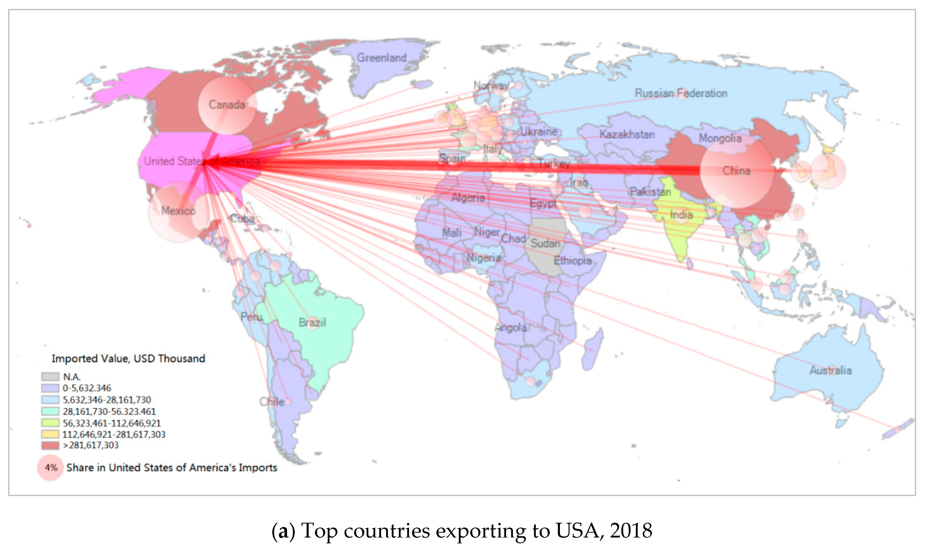
Figure 4a,b shows the U.S.’s top import and export trading partners in 2018. In Asia, the top three were China, Japan, and South Korea. Canada and Mexico were the top two in North America. In Europe, the United Kingdom, Netherland, Spain, Italy, and Belgium were major traders. In South America, Venezuela, Columbia, and Brazil were the leading three. In the Middle East, Saudi Arabia, Egypt, and Iraq were the leading partners. China, Japan, Canada, Mexico, and Venezuela were the top countries with large international trades with the U.S. during the period of 2008 to 2018.

5.1. Top Domestic and International Ports

For the port-level maritime freight per the Census Bureau [1],

Table 3. Top 20 American ports in imports and exports or other measures (1000 tons), 2018.

Rank	Port Name	Total	Domestic	Foreign	Imports	Exports	D/F	I/E
1	South Louisiana, LA, Port of	2,239,874	1,125,501	1,114,373	472,697	641,676	1.01	0.74
2	Houston, TX	2,122,079	658,083	1,463,996	920,190	543,807	0.45	1.69
3	New York, NY and NJ	1,534,802	623,789	911,014	714,602	196,412	0.68	3.64
4	Long Beach, CA	802,053	129,343	672,710	451,861	220,849	0.19	2.05
5	Corpus Christi, TX	767,862	214,310	553,552	433,737	119,815	0.39	3.62
6	New Orleans, LA	730,111	365,298	364,813	195,825	168,988	1.00	1.16
7	Beaumont, TX	694,835	226,879	467,956	411,679	56,278	0.48	7.32
8	Mobile, AL	676,355	295,241	381,114	238,063	143,051	0.77	1.66
9	Plaquemines, LA, Port of	637,443	358,129	279,314	81,498	197,816	1.28	0.41
10	Los Angeles, CA	597,883	68,751	529,133	327,328	201,805	0.13	1.62
11	Lake Charles, LA	537,781	220,118	317,664	260,089	57,575	0.69	4.52
12	Texas City, TX	526,060	138,956	387,104	339,266	47,838	0.36	7.09
13	Baton Rouge, LA	518,095	359,087	159,008	108,852	50,157	2.26	2.17
14	Duluth-Superior, MN and WI	453,418	303,325	150,093	4,860	145,233	2.02	0.03
15	Norfolk Harbor, VA	445,931	77,067	368,864	95,768	273,095	0.21	0.35
16	Baltimore, MD	434,127	124,541	309,586	166,131	143,455	0.40	1.16
17	Tampa, FL	396,761	262,964	133,797	76,773	57,024	1.97	1.35
18	Paulsboro, NJ	363,517	124,819	238,698	223,045	15,653	0.52	14.25
19	Savannah, GA	353,937	18,387	335,550	195,844	139,706	0.05	1.40
20	Pascagoula, MS	335,898	94,525	241,373	190,628	50,745	0.39	3.76

shows U.S. trade freight flows by weight at 20 selected major U.S. ports. South Louisiana, LA; Houston, TX; New York, NY; and New Jersey, NJ were the largest ports for U.S. imports and exports, and for domestic freight. Some ports played a balanced role for imports and exports with an I/E ratio close to 1.00 (i.e., New Orleans, Baltimore), whereas others were skewed toward either to import (i.e., Texas City, Paulsboro, Philadelphia, Freeport) with an I/E ratio > 7.00 or export (i.e., Duluth-Superior, Portland) with an I/E ratio < 0.30. Similarly, some ports provided different contributions to foreign (imports + exports) or domestic freight. The ports of South Louisiana and New Orleans were balanced in domestic and import/export with a D/F ratio close to 1.00, whereas ports of Savannah, Los Angeles, and Long Beach were primarily for import/export with a D/F ratio < 0.20, and ports of Baton Rouge and Duluth-Superior were mainly for domestic goods with a D/F > 2.00.

According to the U.S. Bureau of Transportation Statistics [7], the top 25 U.S. ports by total weight in tonnage and by TEU, including import, export, and domestic, are shown in Figure 5a,b. These top ports in Figure 4a handled two-thirds of U.S. import and export trade weight in 2017, including bulk freight, such as coal, petroleum, and grain. About 90% of U.S. import and export maritime TEUs in 2017 were shipped at these top ports (Figure 4b).

Table 4. Top 20 foreign ports by five-year total freight weight (billion tons), 2014–2018.

Rank	Port	Country	2018	2017	2016	2015	2014	Total
1	Shanghai	China	50.80	56.14	53.70	44.30	37.90	242.84
2	Singapore	Singapore	51.54	48.36	44.85	42.33	39.34	226.42
3	Rotterdam	Netherlands	42.11	40.12	37.84	37.66	35.26	192.99
4	Ningbo	China	36.19	47.16	30.97	27.24	22.59	164.14
5	Guangzhou	China	34.70	34.14	30.28	24.17	21.52	144.81
6	Tianjin	China	36.52	30.95	25.76	24.51	20.62	138.35
7	Hong Kong	China	25.94	24.54	23.82	23.01	22.09	119.41
8	Busan	South Korea	24.17	24.36	21.79	21.72	21.98	114.01
9	Qingdao	China	27.83	26.50	22.42	18.43	16.17	111.34
10	Qinhuangdao	China	25.20	24.60	20.49	16.75	15.03	102.07
11	South Louisiana	United States	20.32	20.78	20.46	19.25	20.35	101.16
12	Nagoya	Japan	21.81	21.56	20.80	18.71	18.23	101.11
13	Dalian	China	24.60	22.29	20.05	17.68	14.52	99.13
14	Houston	United States	19.25	19.60	20.15	19.20	18.34	96.54
15	Antwerp	Belgium	18.94	18.29	16.74	16.01	15.23	85.21
16	Shenzhen	China	18.70	19.92	17.60	15.39	13.52	85.14
17	Ulsan	South Korea	17.03	16.87	16.11	1.04	15.65	66.69
18	Port Hedland	Australia	15.94	13.07	11.18	11.06	10.85	62.10
19	Klang	Malaysia	15.23	13.55	12.20	10.97	9.99	61.95
20	Dampier	Australia	14.08	13.39	12.60	11.01	0.88	51.97

lists the top 20 world ports in freight handling, including import and export sorted by five-year total freight weight (billon tons) for the period of 2014–2018 [1,7]. Shanghai, China was ranked at the top with 242.84 billion tons, with Qinhuangdao, China ranked in the middle, and Dampier, Austria ranked 20th. China had nine ports in the top 20; the U.S. and South Korea each had two ports. Asia, as a whole, held 14 of the top 20 ports, with Europe and Australia each having two ports. Notably, Singapore was ranked 1st in 2014 and 2018 in total port throughput freight.

The 50 largest international ports in handling global container freight volume in TEUs are shown in Figure 6. These ports are located over six continents, in 200+ countries, and connect the world maritime shipping routes. They are highlighted in dark blue in the background of oceans, with route width representing flow volume [38]. Most of these ports are located in Asia, Southeast Asia in particular; the Middle East; and Europe. Africa only has one such top port [30]. Please note that the maritime network containing dark blue lines connecting the top ports and other smaller ports does not really exist. It is just an abstract representation of likely corridor spaces that the majority of individual vessels may go through between ports. Refer to Section 5.3 for more discussions.

5.2. Maritime Freight Flow Highlights

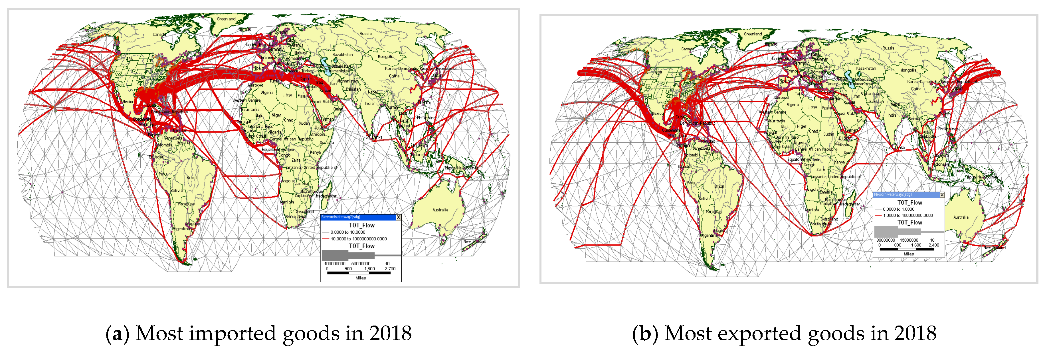
Assigned maritime flows between any two global sea ports are optimal flows based on AON assignment, which assumes no capacity limits at ports and one ocean routes. As such, U.S. export freight from one port is completely assigned to the port in another country that is the closest through all possible ocean routes connecting the two ports. The same assignment also applies to U.S. import freight from a foreign port to a U.S. port. The resulting freight flows are highlighted with the route width representing flow volume: the thicker the width, the higher the freight volume on the route.

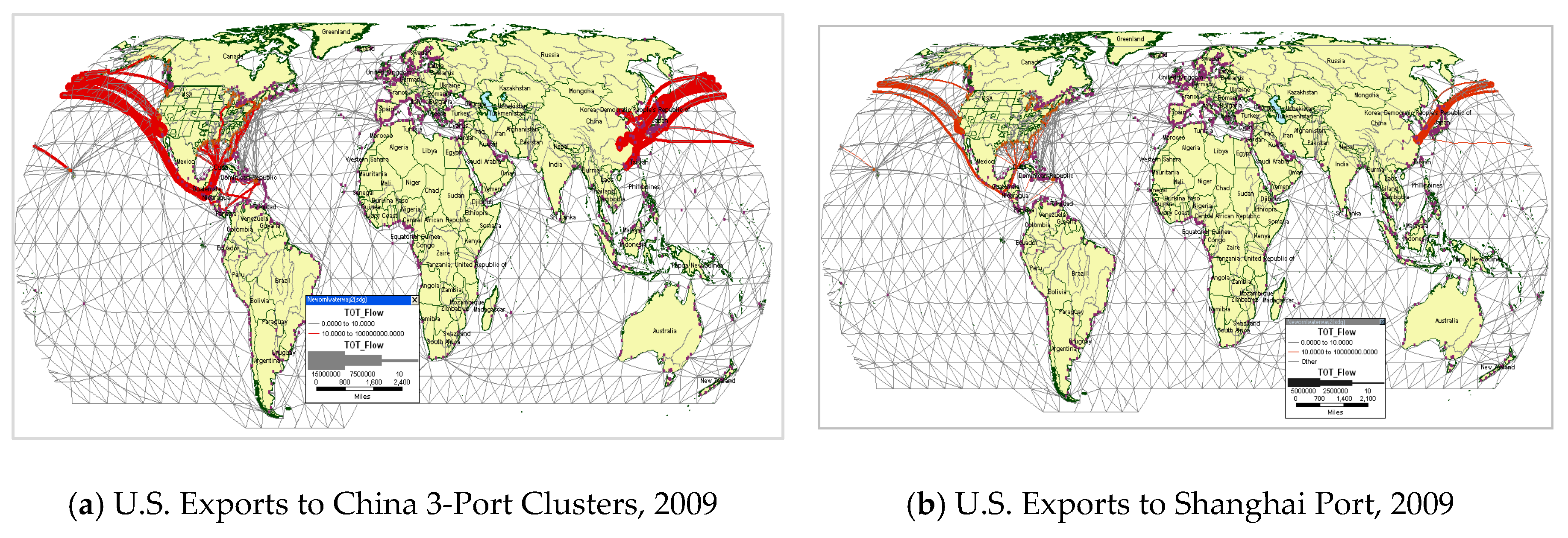
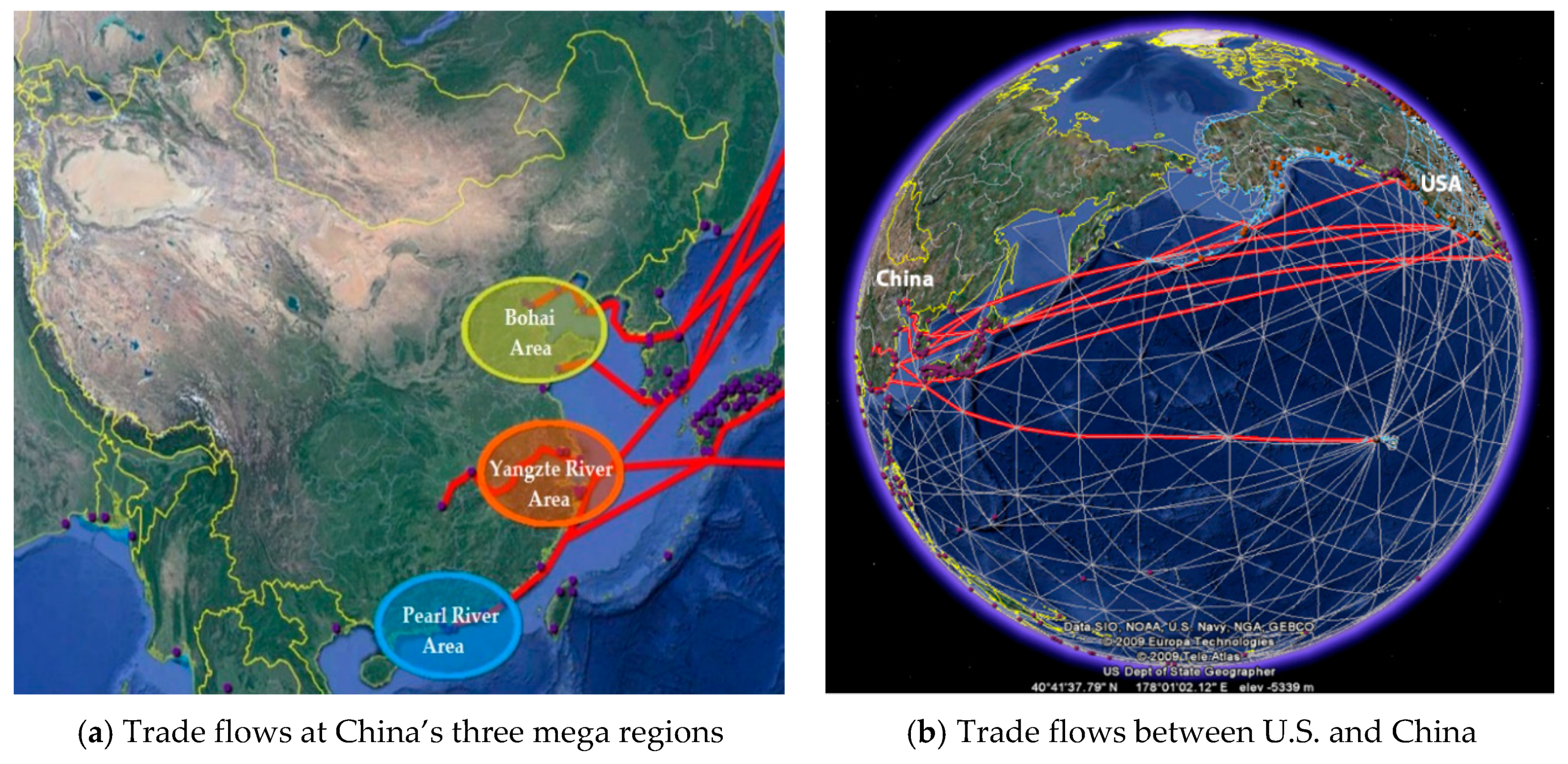
Figure 7, Figure 8 and Figure 9 depict optimal routing for U.S. exported and imported goods in 2009 or 2018; the total commodity for the world shown in Figure 6 and that for U.S. coastal ports is shown in Figure 7c,d. Specific commodities, such as most traded goods, are shown in Figure 8a,b. Finally, trade flows between specific country ports such as China and USA are illustrated in Figure 9a for U.S. exports to China’s three megaregion ports and in Figure 9b to the Shanghai port only in 2009. These selected maps provide snapshots of U.S. import and export freight flows with foreign ports at the world, country, port, and commodity levels.

Visually, the Panama Canal, which links ports in countries around the Atlantic Ocean and the Pacific Ocean, and the Suez Canal, which connects ports in countries near the North Atlantic Ocean and Northern Indian Ocean, are strategically important for international freight shipments to and from the United States.

Mega regions are characterized by a social, economic, and spatial expansion of population, commerce, transportation, and resources across a geographical space; and a total population count exceeding 10 million residents whom are spread among several urban areas in close proximity [39]. With increasing urbanization and globalization, mega regions play important roles in international trade. Figure 10 summarizes some key characteristics of three major mega regions in China. China has been one of the top three trade partners with the U.S. The three mega regions together contributed over 87% of China’s exports to the USA in 2009, as shown in

Table 5. Top Indictors by port clusters in Bohai, Yangtze River, and Pearl River areas, 2009.

Major Indictors	Pearl River Delta Area	Yellow River Area	Bohai Bay Area	Four Area Total	Total in or % of China
Area (km)	109,285	110,821	225,713	445,819	12.4%
Population in 10,000	7165	9723	12,180	29,068	22.0%
GDP in RMB 100 M	33,627	43,235	46,488	123,350	50.0%
FDI in USD $10,00	3,652,965	8,129,562	4,767,428	16,639,955	79.0%
Population Density	656	877	540	652	178
GDP Per Capita	46,932	44,467	38,168	42,435	227.4
Freight in USD $100 M	6860	7787	4337	18,984	87.00%

. This percentage has been rising during the period of 2008–2018.

Global freight flows of U.S. international trade in 3D were implemented in Google Earth with optimal assignment results from TransCAD, and shown in Figure 9; the total U.S.–China imports and exports flows at China’s three major port clusters or mega regions in 2009 are shown in Figure 10a; and the total U.S.-China imports and exports flows over the Pacific Ocean, including Hawaii, are shown in Figure 10b. Note that the mash network for maritime freight flows was overlain onto the Google Earth to strengthen the visual 3D effects in Figure 9b. The red lines represent the optimal links and routes carrying freight flows between U.S. and China.

5.3. Visual Validation

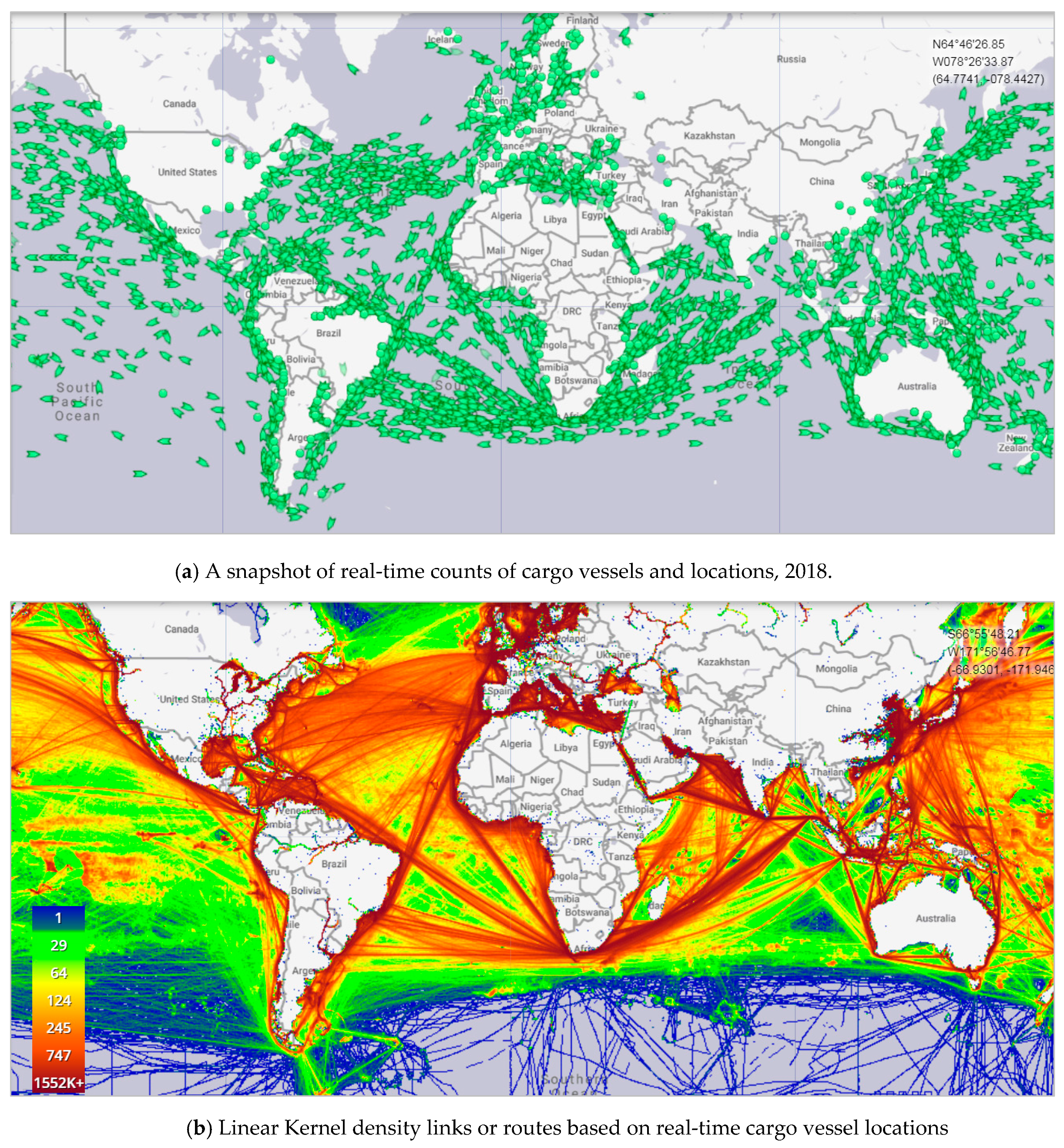
Validating flow movement through a transportation network normally involves nodal and link/path flow validation. However, in this research the freight flows at origin and destination ports are given and assigned to the maritime network. With flow conservation at ports, nodal flow validation is not needed. Flows at ports can be directly used to rank and highlight to show the top ports and their import and export flows. To validate flows on links and/or paths, one way is to compare the model results with known maritime freight flows, ideally using the same unit (i.e., TEU) for the same time period on the same link or route. However, to validate this way is non-trivial for maritime freight flows because maritime network ports are fixed in location, size, and capacity while maritime network links or routes are not physically fixed. By comparison, a maritime network is different from a highway network, which has fixed links and routes, and is similar to an air transportation network, which has no fixed links or routes. Having no fixed links and routes makes it hard to get flow samples for links or routes to validate any maritime network, especially when the fixed maritime ports as ODs have known freight production and attraction flows. Therefore, we validate roughly using a visual approach by comparing assigned mash network links and routes with the actual vessel density network derived from real-time vessel locations.

For example, Figure 11a shows real-time counts of maritime cargo vessels tracked in 2018 [40]. In the map, the green dots are ports and the green ship-shapes are vessels, which were carrying imported or exported goods in all directions to their world destination or transfer ports, including U.S. sea ports. However, if we process vessels by their locations as points using the linear Kernel density function in GIS, we get Figure 11b, which visually provides port-port maritime links and routes ranging from low density of 1 (dark blue) to high density 1552 (in dark brown). The high-density points form imaginary links and routes, which together can be regarded as or drawn as a maritime network. Clearly, we can visually compare Figure 11b with Figure 5, which shows major links and routes of a global container maritime network, and Figure 7a,b, which shows modelled total import and export results assigned on the mash network connecting 4000+ ports in 200+ countries in this study. Obviously, the links and routes that carry resulting optimal flows in 2018 are quite similar to the density networks, not only for the world, but also more so around the United States, as Figure 5 and Figure 11a,b illustrate major corridors and density links and routes for all vessels heading to all directions, while Figure 7a,b only depicts maritime links and routes importing to and exporting from the United States. For example, the maritime flow routes in Figure 7a,b do contain flows between Brazil and Europe, South Africa and the Middle East, South Africa and Southeast Asia, and Southeast Asia and the Middle East. Other than visual validation, other ways, such as aggregated real-time tracking to the same temporal unit, meta-analysis with recorded or reported data from other reliable sources, or simulations with acceptable statistical accuracy metrics, may be developed to further validate the model framework and the results by comparing flow volumes on selected links or routes of the same maritime network. Obviously, all these and other validation possibilities warrant more follow-up studies.

6. Conclusions and Remarks

In this study, we concisely reviewed publicly available import and export databases for U.S. and the world maritime freight; developed an integrated model consisting of data mining (DM), linear programming (LP), and AON transportation assignment models through integration of software packages, including ArcGIS, TransCAD, and Google Earth; and visualized the U.S. global maritime import and export freight flows. This integrated model provides an alternative yet novel method to capture and highlight U.S. maritime trade patterns. The source databases were identified and selected from various public agencies, and the target database with desired attributes was obtained through using data mining and integration. Important issues, such as spatial scales, measurement units, conversions, code matches, and data manipulations, were discussed. Overall, we focused more on integration and result visualization than Shen [24,25], who emphasized data mining and processing.

Major U.S. trade patterns in terms of freight flows at the world, country, mega region, and port levels were highlighted. Representative ports and freight routes for total or specific and for the most or the least goods by weight, value, and TEU were listed or visualized. Sample optimal flows for U.S. global maritime freight for U.S.–World and U.S.–China were shown in 2D maps drawn using TransCAD and 3D maps in Google Earth.

The major contributions of this study include the development of an integrated model framework consisting of DM for mining possible source databases, LP for the target database with attributes from the best candidate databases, and AON for system-wide optimal assignments. The visualization of the best maritime links and routes for total goods and specific commodities between any country and the United States is a novel contribution, especially in terms of scale of 4000+ ports, 200+ countries, large maritime networks, and types of goods. The specific highlights of maritime trade links and routes in 2D and 3D between the world’s top two economies, the United States and China, are also innovative. The visual validation of optimal links or routes of the modelled maritime network against the density network from real-time vessel locations is creative, yet better to be further validated with flow volumes on links and routes. Overall, the findings reveal important maritime routes or corridors between a foreign country and the United States, providing a baseline for studying various international trade, shipping, and geo-political issues. The integrated model framework is also transferrable to study maritime freight movement in other countries.

The findings could be enhanced in several directions. First, finer temporal units could be used for more detailed freight flows analyses. This would require seasonal, monthly, weekly, daily, or even real time to be used rather than yearly data. This point is perhaps particularly relevant to carriers/shippers who can cooperate on vessels/routes and consider price premiums for holiday seasons the similar way as the ridesharing and surge pricing on urban travel demand [41]. More detailed studies are expected to lead a better understanding of U.S. maritime imports and exports dynamics. Second, the U.S. international freight flows are complex in reality, with some ports being more important in trade than others, indicating a hierarchical hub-spoke network system over time. Third, the visualization of spatial elements, such as country boundary, port location, network configuration, and flows is largely in 2D, whereas 3D visualization is comparatively advantageous. Fourth, since the U.S. maritime import and export flows at ports must connect to demand and supply locations, the linkage of maritime ports to the demand and supply locations through intermodal networks warrants further research. Fifth, the modelled results in terms of optimal flows and routes require further validation and reliability checks for future applications, even though ocean routes are rarely fixed and link capacities are hard to specify. Finally, model simulations could be conducted under special situations; e.g., shut-down or capacity doubling at key ports or on critical routes; fast economic development, e.g., commodity supply or demand from a particular country or region; or extreme events, e.g., hurricane, outbreak, or terrorist attack.