Water Areas Segmentation from Remote Sensing Images Using a Separable Residual SegNet Network

Abstract

Changes on lakes and rivers are of great significance for the study of global climate change. Accurate segmentation of lakes and rivers is critical to the study of their changes. However, traditional water area segmentation methods almost all share the following deficiencies: high computational requirements, poor generalization performance, and low extraction accuracy. In recent years, semantic segmentation algorithms based on deep learning have been emerging. Addressing problems associated to a very large number of parameters, low accuracy, and network degradation during training process, this paper proposes a separable residual SegNet (SR-SegNet) to perform the water area segmentation using remote sensing images. On the one hand, without compromising the ability of feature extraction, the problem of network degradation is alleviated by adding modified residual blocks into the encoder, the number of parameters is limited by introducing depthwise separable convolutions, and the ability of feature extraction is improved by using dilated convolutions to expand the receptive field. On the other hand, SR-SegNet removes the convolution layers with relatively more convolution kernels in the encoding stage, and uses the cascading method to fuse the low-level and high-level features of the image. As a result, the whole network can obtain more spatial information. Experimental results show that the proposed method exhibits significant improvements over several traditional methods, including FCN, DeconvNet, and SegNet.

1. Introduction

Lakes and rivers are the interactive connecting points of atmosphere, biosphere, lithosphere, and land hydrosphere [1]. They are extremely sensitive to climate changes, and thus are able to reflect not only regional and global climate changes, but also local temperature changes [2]. Therefore, the study of lake and river changes is great significance to the study of global climate changes. The segmentation of lakes and rivers is an important first step to study their changes. Traditional methods of water area segmentation mainly include thresholding, clustering, support vector machine, and so on. McFeeters et al. [3] proposed a normalized difference water index (NDWI). This method uses the combination of an image’s green band and near-infrared band to construct a wave band for segmentation, but this method is highly dependent on the environment. In 2000, Frazier et al. [4] classified the water body of the river beach based on maximum likelihood classification, but his method’s generalization performance is poor, because there are obvious differences in different infrared band images. Yuan et al. [5] proposed a new spatial constraint model driven clustering method, which clusters candidate objects through sparsity, but this method is limited by the image’s spatial resolution. Lu et al. [6] used threshold segmentation to analyze multispectral satellite images, but the spectra deference in different regions has great influence on the segmentation accuracy. Zhang et al. [7] proposed a support vector machine method to perform the coastline extraction by minimizing errors and maximizing geometric edge features, but it has difficulties in large scale data training. Feyisaet et al. [8] proposed the automatic water area segmentation index (AWEI), which significantly improves the segmentation accuracy of shadow area and dark surface, but its extraction ability on small targets is not good. Michael et al. [9] proposed the tandem-x coastline extraction based on non-local filtering. This method has a good effect on coastline extraction, but it misses small targets within the coastline. Du et al. [10] designed a new method for surface water detection based on a digital elevation model (DEM), which achieves a high accuracy. However, the problem is that different infrared images have a great influence on the results. Park et al. [11] proposed a density based spatial clustering (DBSCAN) algorithm, but there are obvious differences in the extraction between the bright and shadow parts of the image. In the same year, Wang et al. [12] proposed a new method by combining the NDWI with the image segmentation method. Cheng et al. [13] used an adaptive neighborhood selection method to extract water body and buildings from remote sensing images. To summarize, the above methods for water area segmentation all have high requirements for data processing and exhibit poor generalization performance, that is, they cannot extract arbitrary lakes and rivers accurately.

Since the rise of artificial intelligence, deep learning has been widely used in speech recognition, image recognition, information retrieval, and other fields [14]. Compared with traditional segmentation methods, the deep learning method does not require any prior conditions to perform automatic water area segmentation from remote sensing images. With the increase of computing power and the emergence of GPUs, more and more convolutional neural network (CNN) models have been proposed, such as the visual geometry group network (VGGNet) [15], the googLe network (GoogLeNet) [16], the densely connected convolutional network (DenseNet) [17], and so on. The classification accuracy of these neural network models has reached the human level. The neural network method can extract deep features of remote sensing images to achieve better classification [18], e.g., in water area segmentation. However, CNN models can only classify a specific object, but lack the ability to extract its accurate location and boundary information. Therefore, for remote sensing images, such as of lakes and rivers, which have high requirements for location and boundary extraction, the traditional CNN models are not accurate enough. To solve this problem, a semantic segmentation model which can achieve pixel-level classification has been proposed in recent years.

The Semantic segmentation algorithm can classify images at the pixel level and extract more detailed features. The algorithm’s high precision and fast speed make a hot research topic in image segmentation. In 2014, Long et al. [19] proposed a fully convolutional network (FCN) for semantic segmentation, in which, the last two fully connected layers of the VGGNet are changed to fully convolutional layers and skipping connection is used to realize an end-to-end and pixel-to-pixel deep neural networks (DNN). In the same year, the decovolution network (DeconvNet) was proposed by Noh et al. [20], who used a new method for upsampling: deconvolution. However, an image’s fine granularity cannot be fully displayed by DeconvNet, and the network’s understanding of features is not sufficient. In addition, because there are too many convolution kernels, the model’s parameter number is large and its calculation burden is high. In 2015, Badrinarayanan et al. [21] also proposed a semantic pixel-wise segmentation network (SegNet) based on the VGGNet. SegNet makes full use of the location index information during convolution process, greatly reducing the memory consumption, but this technique also increases the training time and reduces the efficiency. In 2017, a pyramid scene parsing network (PSPNet) was designed by Zhao et al. [22] which applies dilated convolution [23] to convolution layers, increasing the receptive field without increasing the number of parameters. Nowadays, more and more semantic segmentation algorithms based on deep learning are proposed. These algorithms have great prospects in processing remote sensing satellite images and segmenting pathological cells in medical images and other fields. Although existing semantic segmentation algorithms perform well in remote sensing image extraction, there is a problem of gradient vanishing due to the deepening of convolution layers during training process, and thus the network performance degrades and its image segmentation accuracy is affected. In addition, a DNN normally has many convolution kernels, which increases the parameter numbers of the training network, and thus makes the training time-consuming and difficult [24]. To solve these problems, a separable residual SegNet (SR-SegNet) is proposed in this paper. A modified residual block is added to the encoder of SegNet to solve the problem of performance degradation. Furthermore, depthwise separable convolutions [25] are introduced to reduce the parameter number, shorten the training time, and cut down the calculation cost without compromising the network performance. In the proposed network, the characteristics of high-level (the higher layer of deep neural network layer) and low-level (the lower layer of deep neural network layer) are obtained by cascading. In addition, dilated convolutions are used to expand the receptive field in convolution layers to improve the ability of feature extraction without increasing the number of parameters. Compared with FCN, SegNet, and DeconvNet, the SR-SegNet proposed in this paper improves the F1-score, mean intersection over union (Miou), and recall, while also reducing the testing time.

The remainder of this paper is organized as follows. In Section 2, the structure of SR-SegNet is discussed in detail. Section 3 presents experimental details of the proposed model using Lake and River dataset. In Section 4, conclusions are given and the future research direction is discussed.

2. Proposed Method

In this section, the proposed SR-SegNet’s architecture is presented in detail. The classical SegNet uses a large number of convolution kernels and a deep network structure to extract image features, thus its training is slow, and vanishing gradient (vanishing gradient: as the number of neural network layers increases, the accuracy of classification decreases) always happens. The segmentation of lakes and rivers in remote sensing images is limited by the images’s spectrum, resolution, shadow, and other factors. In addition, there are some problems in the application of traditional methods, such as poor generalization performance, poor effect of water area segmentation, and so on. In this paper, we propose a SR-SegNet to solve these problems; the method can retrieve rich and multi-scale contexts for a more accurate segmentation, and significantly decrease the number of training parameters and reduce the image prediction time.

2.1. Model Overview

The classical SegNet has a large number of parameters. Therefore, vanishing gradient always happens and its ability of feature extraction deteriorates during training process. Its parameter number is large because there are too many convolution kernels. Moreover, five times of 2× upsampling are performed during encoding stage, resulting in a long training and a slow testing. In addition, because the classical SegNet simply performs upsampling during encoding stage, it lacks the fusion of high-level and low-level semantic information; as a result, detailed location information could be lost during the segmentation of water area remote sensing image. To solve these problems, we propose a separable residual SegNet. In SR-SegNet, a modified residual block [26] is introduced in the encoding stage, and the detailed information is presented in Section 2.2.1. To limit the parameter numbers associated with a large number of convolutional kernels, we use depthwise separable convolutions for efficiency. Finally, dilated convolutions are applied in our encoder to capture more water area spatial information. More details of the depthwise separable convolution can be found in Section 2.2.2.

Figure 1 shows the detailed architecture of the proposed SR-SegNet. The entire network is divided into two parts: the encoder and the decoder. (1) In the encoding stage, a modified residual block is added to each convolution block to alleviate the degradation problem that often occurs in training process [27]. (2) Considering that the training process is complicated by a large number of parameters, we only perform four times of upsampling during encoding stage, instead of five times of 2× upsampling in the classical SegNet. We also remove the last five convolution layers in encoding stage. (3) To obtain detailed location information of a water body in a remote sensing image, a cascade method is used to fuse (add) both the deep and shallow features of the image. (4) Furthermore, to simplify the network, depthwise separable convolutions [25] are introduced to convolution layers in encoding stage to reduce the amount of computation and the number of parameters during training process. Based on the above four techniques, SR-SegNet v1 is constructed. (5) Because some 3 × 3 convolution kernels are replaced with 2 × 2 convolution kernels in the modified residual block, the receptive field is reduced to a certain extent, and hence the boundary extraction of an individual water body is not good. To solve this problem, SR-SegNet v2 with dilated convolutions is also proposed. Experiments prove that v2 achieves good results, demonstrating the effectiveness of dilated convolutions.

Table 1. The detailed information of proposed SR-SegNet v2.

Name	Kernel Size	Stride	Dilated Rate	Output Size
Down-sampling network
Input	-	-	-	512 × 512 × 3
Conv_1	3 × 3	1	-	512 × 512 × 64
ResBlock_1	2 × 2/2 × 2/1 × 1	1	2	512 × 512 × 64
Add_1	-	-	-	512 × 512 × 64
Pooling_1	2 × 2	2	-	256 × 256 × 64
Conv_2	3 × 3	1	-	256 × 256 × 128
ResBlock_2	2 × 2/2 × 2/1 × 1	1	2	256 × 256 × 128
Add_2	-	-	-	256 × 256 × 128
Pooling_2	2 × 2	2	-	128 × 128 × 128
Conv_3	3 × 3	1	-	128 × 128 × 256
Conv_4	3 × 3	1	-	128 × 128 × 256
ResBlock_3	2 × 2/2 × 2/1 × 1	1	2	128 × 128 × 256
Add_3	-	-	-	128 × 128 × 256
Pooling_3	2 × 2	2	-	64 × 64 × 256
Conv_5	3 × 3	1	-	64 × 64 × 512
SepConv_1	3 × 3/1 × 1	1	-	64 × 64 × 512
ResBlock_4	2 × 2/2 × 2/1 × 1	2	2	64 × 64 × 512
Add_4	-	-	-	64 × 64 × 512
Pooling_4	2 × 2	2	-	32 × 32 × 512
Conv_6	3 × 3	1	-	32 × 32 × 512
SepConv_2	3 × 3/1 × 1	1	-	32 × 32 × 512
ResBlock_5	2 × 2/2 × 2/1 × 1	2	2	32 × 32 × 512
Add_5	-	-	-	32 × 32 × 512
Pooling_5	2 × 2	2	-	16 × 16 × 512
Up-sampling network
UpSampling_1	4 × 4	2	-	64 × 64 × 512
Add_1U	-	-	-	64 × 64 × 512
Conv_1U	3 × 3	1	-	64 × 64 × 256
UpSampling_2	2 × 2	2	-	128 × 128 × 256
Add_2U	-	-	-	128 × 128 × 256
Conv_2U	3 × 3	1	-	128 × 128 × 256
Conv_3U	3 × 3	1	-	128 × 128 × 256
Conv_4U	3 × 3	1	-	128 × 128 × 128
UpSampling_3	2 × 2	2	-	256 × 256 × 128
Add_3U	-	-	-	256 × 256 × 128
Conv_5U	3 × 3	1	-	256 × 256 × 128
Conv_6U	3 × 3	1	-	256 × 256 × 64
UpSampling_4	2 × 2	2	-	512 × 512 × 64
Add_4U	-	-	-	512 × 512 × 64
Conv_7U	3 × 3	1	-	512 × 512 × 64
Conv_8U	1 × 1	2	-	512 × 512 × 2
Output	-	-	-	512 × 512 × 2

shows the detailed information of the proposed SR-SegNet v2. The input is a water body remote sensing image with three channels (red, green, and blue), and the output is a binary segmentation map in which the pixel in gray denotes the water body and the pixel in black denotes the background.

2.2. Encoder Design

2.2.1. Modified Residual Block

The residual block, proposed by He K et al. [26] in 2015, aims at solving the problem that training error increases as the network deepens, and helping alleviate the problems of vanishing gradient and exploding gradient. Inspired by the residual block, to further address the problem of small object misidentification in segmentation of water area remote sensing images, a modified residual block is added to the proposed SR-SegNet in the encoder. As shown in Figure 2a, it is a traditional bottleneck block in ResNet-50. This method protects information integrity by bypassing the input to the output directly. The residual block in ResNet-50 only needs to learn the difference between the input and output; this setup simplifies the learning objectives and reduces the difficulties, and thus solves the degradation problem during training process [28]. The residual block is especially suitable for small and medium-sized object recognitions in water body remote sensing images. However, using 1 × 1 convolution kernels in the traditional bottleneck block may lose the semantic information of water body. For better performance, two successive 2 × 2 convolution kernels are adopted in our modified residual block in this paper, and then a 1 × 1 convolution kernel is connected to them. To enlarge the receptive field to obtain more water body features without increasing the number of parameters, 2 × 2 dilated convolutions with a dilation rate of 2 are introduced into the first two layers of the modified residual block, which generates the same receptive field as 3 × 3 convolution kernels.

In this paper, dilated convolutions are added to the modified residual block during encoding stage, as shown in Figure 2b. In the modified residual block, 3 × 3 convolution kernels are changed to 2 × 2 convolution kernels, which reduces the training complexity of network and saves the training time. However, by this structure, detailed information could be lost in the extraction of water body from remote sensing images. To further expand the receptive field during downsampling and further improve edge feature extraction and small targets recognition in water body remote sensing images, this paper proposes SR-SegNet v2 by introducing the dilated convolutions. Note that SR-SegNet v1 does not use dilated convolutions in its modified residual block.

Compared with SR-SegNet v1, SR-SegNet v2 replaces 3 × 3 convolution kernels in its residual block with 2 × 2 dilated convolutions, with a dilation rate at 2. In Figure 2b, the channel number of the first $2\times 2$ convolution layer is twice that of the latter, and the final 1 × 1 convolution kernels use 64, 128, 256, 512, and 512 channels, respectively, for five modified residual blocks in SR-SegNet. According to Equation (1), the receptive field of the standard 3 × 3 convolution kernel is 3, where m is the receptive field size of previous layer, stride is the convolution step size, and K is the convolution kernel size.

$$r=(m-1)\times stride+K.$$

(1)

Figure 3 shows a comparison between a standard convolution and a dilated convolution. As shown in Figure 3c, a standard 2 × 2 convolution is replaced by a dilated convolution with a dilation rate at 2, which is equivalent to put a zero between every adjacent pixels. Similarly, a 3 × 3 convolution kernel with a dilated ratio of 2 is equivalent to a 5 × 5 convolution kernel. Because these filled zeros do not need training, the dilated convolution can substantially expand its receptive field without increasing computational complexity.

Equation (2) is for calculating the receptive field of a dilated convolution, where rate represents the dilation rate, the size of the convolution kernel is K, and the size of the convolution kernel with a dilated convolution is K${}_d$.

$$K_d=K+(K+1)\times (rate-1).$$

(2)

2.2.2. Depthwise Separable Convolution Construction

In the last two convolution blocks of SegNet, 3 × 3 convolution kernels, each with 512 channels, are used in each layer to increase the depth of the network and thus to extract more features. However, this layout produces a large number of parameters, resulting in high computational burden and difficult training. In practice, most of the water body remote sensing images are of medium or even high resolution, and the traditional SegNet will have a slow segmentation. To reduce the number of parameters without compromising the feature extraction, depthwise separable convolutions are introduced into convolution layers. Depthwise separable convolutions can be divided into two parts: depthwise convolutions and pointwise convolutions. Figure 4 is the construction of depthwise separable convolutions. Depthwise convolution refers to spatial dimensional convolutions on each channel of the input tensor, and pointwise convolutions apply standard 1 × 1 convolutions to fuse the output of each channel [29].

Figure 5 is a comparison between a standard convolution and the depth separable convolution. The standard convolution first performs a 3 × 3 × C convolution, then the batch normalization (BN) [30], and finally the nonlinear relu function [31]. Different from traditional convolution methods, the depthwise separable convolution applies a 3 × 3 × 1 depth convolution first, then the batch normalization and the nonlinear relu function, next a 1 × 1 × C point convolution, and last again the batch normalization and the nonlinear relu function. The standard convolution uses the complete 3 × 3 × C convolution kernel directly, but the depth separable convolution uses C single channel 3 × 3 convolution kernels at the same time [32]. For example, if N K × K standard convolutions of C channels each were used, the number of parameters would be NCK${}^2$. However, for the depthwise separable convolutions, KxK depthwise convolutions of C channels each are performed at each channel of the input picture, and thus CK${}^2$ parameters are generated firstly. Next, N 1 × 1 × C pointwise convolutions are used to aggregate outputs, and thus NC parameters are generated. Therefore, the whole depth separable convolutions generates CK${}^2$ + NC parameters, many fewer than that of standard convolutions.

The application of depthwise separable convolutions in water area segmentation not only shortens training time and reduces computation, but also effectively avoids overfitting. Using depthwise separable convolutions makes the model easier to train. Moreover, training and prediction time will also be reduced.

2.3. Decoder Design

Although the end-to-end model can directly use a whole picture as the input and generate a whole picture as the output [33]. Image spatial information could be lost during decoding stage. The U-Net proposed by Ronneberger O et al. [34] uses concatenation in both encoder and decoder to fuse high-level and low-level image features to obtain more feature information.

Previous work shows that the layer by layer upsampling does not improve prediction results, but instead it increases the complexity of model and generates a large number of parameters. Information in encoding layers will be lost if the upsampling is as of the same size as the input image directly. In view of the above situations, our proposed SR-SegNet in this paper combines an end-to-end cascading mode, and adopts 4× unpooling for the first upsampling, instead of traditional 2× unpooling. Next, 2× unpooling is conducted layer by layer. As a result, there are only four times of unpooling. In the residual block of encoder, the first four residual blocks are cascaded with the upsampling in decoding stage. The cascading uses the fusion method to effectively obtain more spatial location information. This method combines high-level and low-level features, and can extract detailed features of water body remote sensing images, especially the edges in them [35].

3. Experiment and Result Analysis

To verify the effectiveness of SR-SegNet proposed in this paper, experiments were carried out on Lake and River dataset. Furthermore, semantic segmentation models were used as the control groups. All experiments were evaluated based on four major metrics, including Accuracy (Ac), Dice, F1-Score (F1), and Mean intersection over union (Miou). Experimental results show that the network proposed in this paper exceeded all comparing networks on the evaluation metrics.

3.1. Data Augmentation

The experimental dataset includes the remote sensing satellite images of Namtso Lake in Qinghai-Tibet Plateau and a river in Central China during 2015–2019 from China Center For Resources Satellite Data and Application (http://www.cresda.com/CN/). After undifferentiated classification, 32 training images and 7 testing images were prepared. Because the water body in an image only accounts for a small part, Adobe Photoshop CS6 software was used to cut the remote sensing image into small pieces 512 × 512 pixels each in size, and Labelme was used for classification and annotation. The lake was classified as Category 1, and the background as Category 2. The cropped images and their corresponding labels are shown in Figure 6a. It is worth noting that there were only pictures of Namtso Lake in the training set, and there was no picture of other lakes or rivers. Furthermore, remote sensing images in the training set and in the test set were not of the same river. To distinguish different rivers, River 1, River 2, and River 3 are used to mark them.

The Deep neural network needs a large number of training data, but it is difficult to obtain these learning samples. Therefore, it is very necessary to use data augmentation to avoid overfitting when there are only a few training samples [36]. Thus, 5000 pictures were generated by scaling, translation, flipping, and rotation. According to a ratio of 7:3, 3750 pictures were divided into training set and 1250 pictures into validation set. Figure 6b shows the images and their corresponding labels after data augmentation.

3.2. Evaluation Metrics

To evaluate the quantitative performance of different models, four evaluation metrics were selected: Accuracy, Dice, F1-Score, and Miou.

$$\begin{array}{cc}\hfill & Ac=\frac{TP+TN}{TP+FP+FN+TN}\hfill \end{array}$$

(3)

$$\begin{array}{cc}\hfill & Dice=\frac{2TP}{2TP+FN+FP}\hfill \end{array}$$

(4)

$$\begin{array}{cc}\hfill & Precision=\frac{TP}{TP+FP}\hfill \end{array}$$

(5)

$$\begin{array}{cc}\hfill & Recall=\frac{TP}{TP+FN}\hfill \end{array}$$

(6)

$$\begin{array}{cc}\hfill & F1=2\times \frac{Precision\times Recall}{Precision+Recall}\hfill \end{array}$$

(7)

$$\begin{array}{cc}\hfill & Miou=\frac{TP}{TP+FP+FN}\hfill \end{array}$$

(8)

where ’Ac’ is defined as the number of pixels correctly classified in a whole picture; ’Dice’ is used to measure the similarity between two pictures; ’Precision’ is the proportion of correctly classified positive pixels to all predicted positive pixels; ’Recall’ is the percentage of correctly classified positive pixels to all true positive pixels; ’F1’ is the combination of accuracy and recall rate; and ’Miou’ is used to describe the accuracy of segmentation [37]. TP is true positive, TN is true negative, FP is false positive, and FN is false negative. The calculation formulas are shown in Equations (3)–(8).

3.3. Experiment Setting and Training

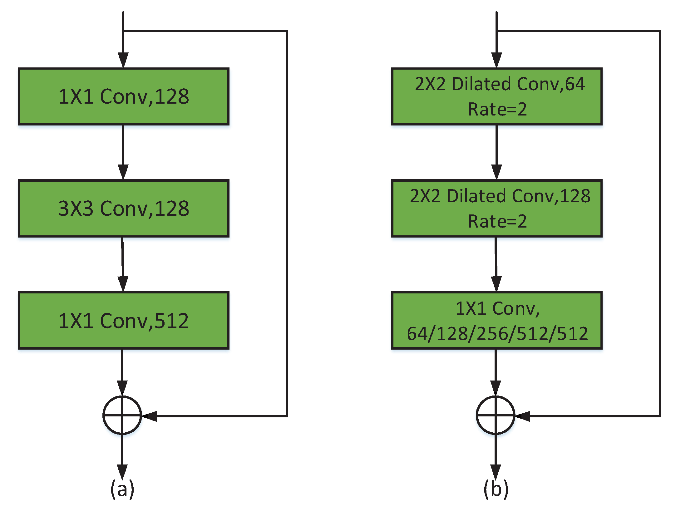
In the experiment, VGGNet was used as the backbone network, and the official VGGNet weights published by keras were used as the pre-training weights. DeconvNet, FCN32s, FCN16s, and FCN8s were selected as the comparison networks. In this paper, SR-SegNet v1 and SR-SegNet v2 are proposed. The residual block of SR-SegNet v1 did not use dilated convolutions, and the residual block of SR-SegNet v2 used 2 × 2 dilated convolutions with a dilation rate of 2. During training phase, the SGD optimizer [38] with an initial learning rate of 0.0001 was used. The momentum was set to 0.9 and the weight decay was set to 0.0005. All models were trained for 300 epochs with a mini-batch size of 2. All experiments were carried out under windows 10 with a AMD Ryzen 7 2700 CPU (3.2 GHz), 16GB of memory (RAM), and a NVIDIA GeForce RTX 2070 (8 GB). Python 3.6 was used and the experiments were based on the keras programming framework. Furthermore, the cross entropy was used as the loss function of neural network, as shown in Equation (9). x${}_i$ represents the sample; p (x) and q (x), respectively, represent two separate probability distributions of random variable x; and n is the number of samples.

$$Loss=\sum _{i=1}^{n}p\left(x_i\right)log\left(p\left(x_i\right)\right)-\sum _{i=1}^{n}p\left(x_i\right)log\left(q\left(x_i\right)\right).$$

(9)

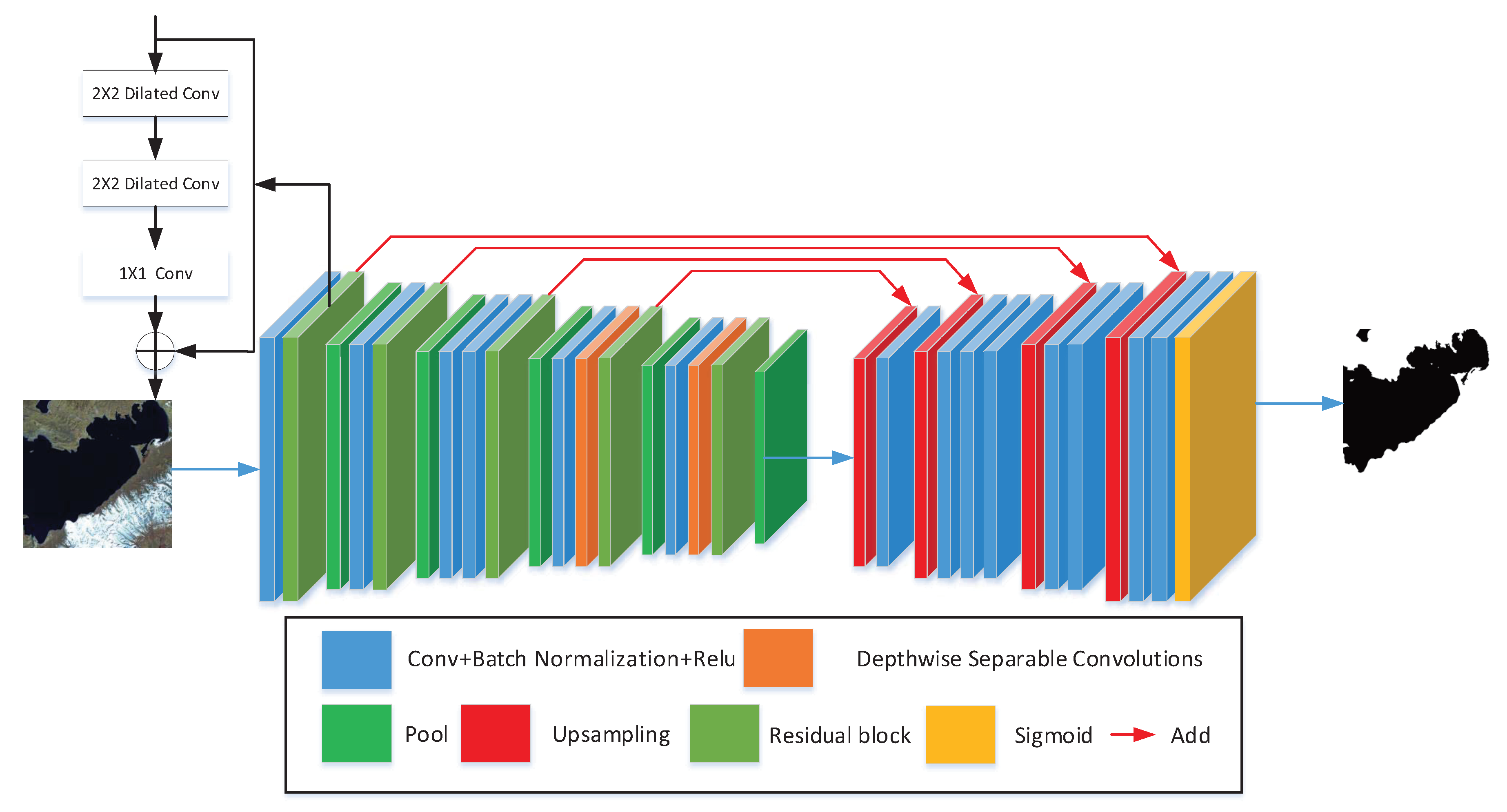
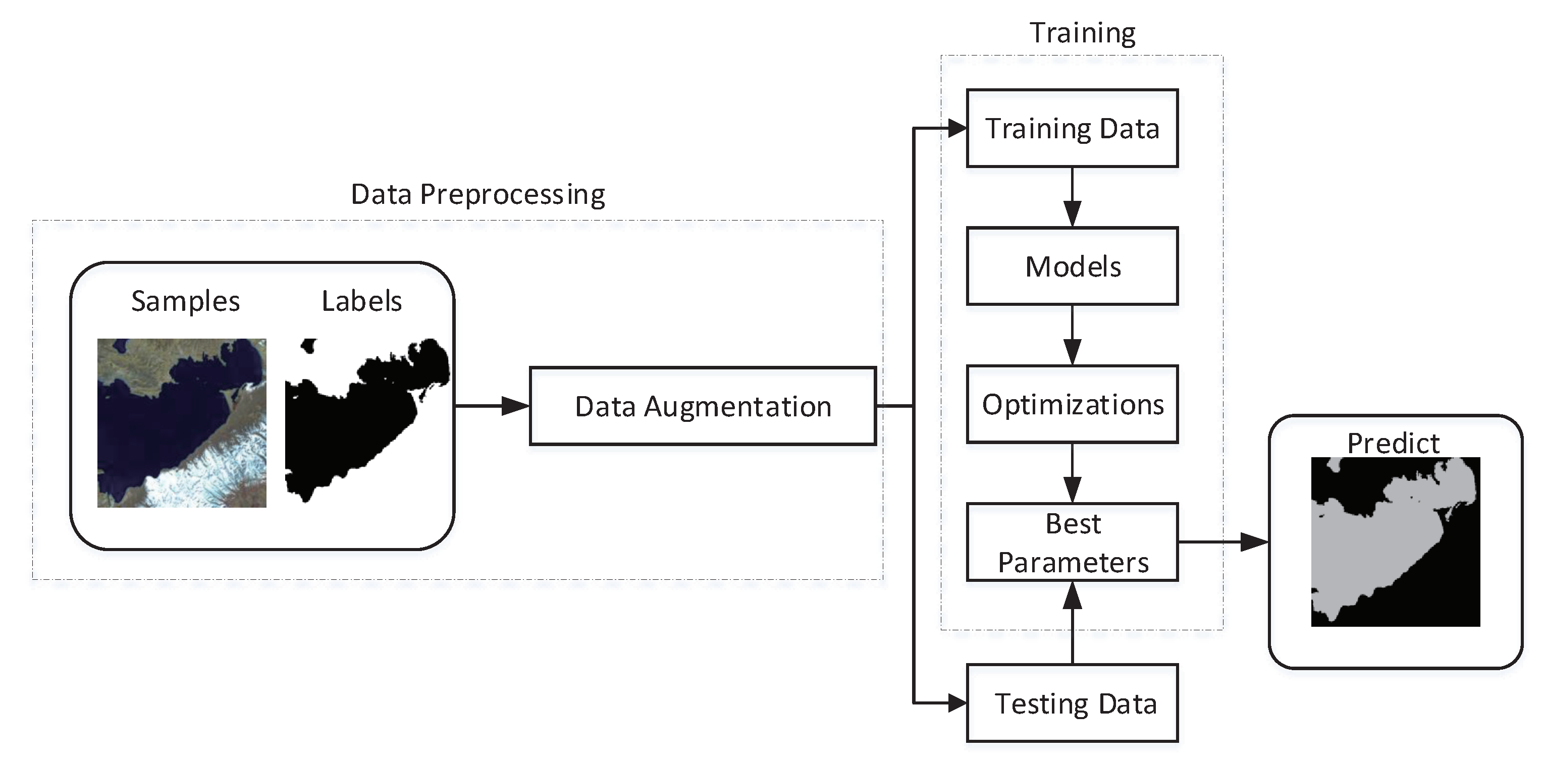
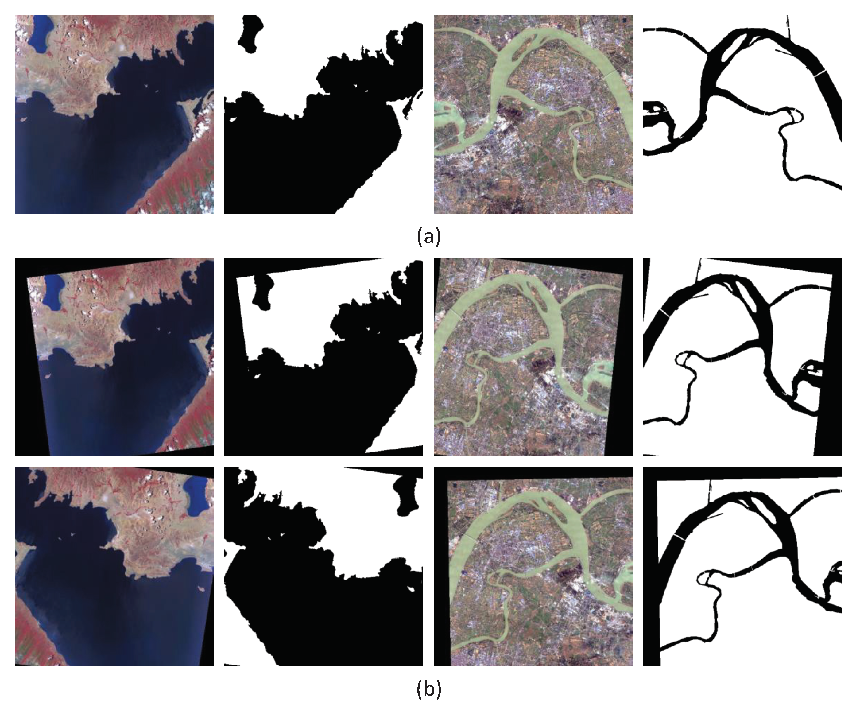
The proposed water area segmentation system is illustrated in Figure 7. First, the Lake and River dataset was preprocessed to generate more data for neural network training through data augmentation; this technique increases the complexity of data and effectively reduces the overfitting of training [39]. Second, the dataset was divided into training set and testing set, and the images from the training set were put into the model for training. The training procedure used the gradient descent algorithm. The labels were compared with predicted results, and the parameters were updated continuously by using back propagation and calculating the loss function [40]. Finally, the model’s optimal parameters were saved to predict and evaluate lake and river images in the testing set.

3.4. Result Analysis

The experiments prove that the proposed SR-SegNet v1 and SR-SegNet v2 in this paper reduce the number of parameters by 65% and 71%, respectively, compared with the classical SegNet, and the training speed of v1 is improved by more than 10%. In addition, the Miou of v2 is improved by 2.37%. The results are shown in

Table 2. Comparison of SR-SegNet and the classical SegNet in training time and parameters.

	SegNet	SR-SegNet v1	SR-SegNet v2
Parameters (M)	29.459	8.5804	10.4172
Training time (h)	100.7	81.3	92.9

and

Table 3. Segmentation metrics of test images in each model. The highest values for the different metrics are highlighted in bold.

	Ac/%	Dice/%	F1/%	Miou/%
FCN32s	88.3	78.74	89.73	68.42
FCN16s	92.49	73.96	90.21	82.95
FCN8s	93.98	75.97	91.56	89.53
DeconvNet	92.98	78.98	88.79	85.86
SegNet	98.86	93.17	99.39	90.85
SR-SegNet v1	99.18	94.47	99.56	93.06
SR-SegNet v2	99.17	94.37	99.49	93.22

.

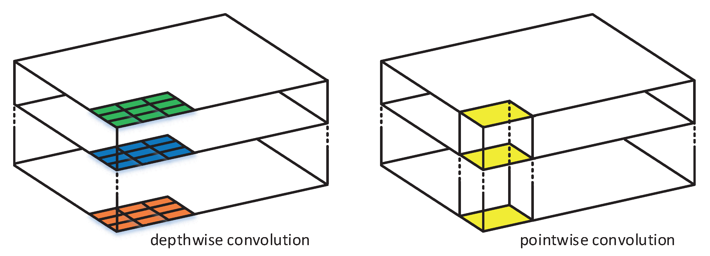
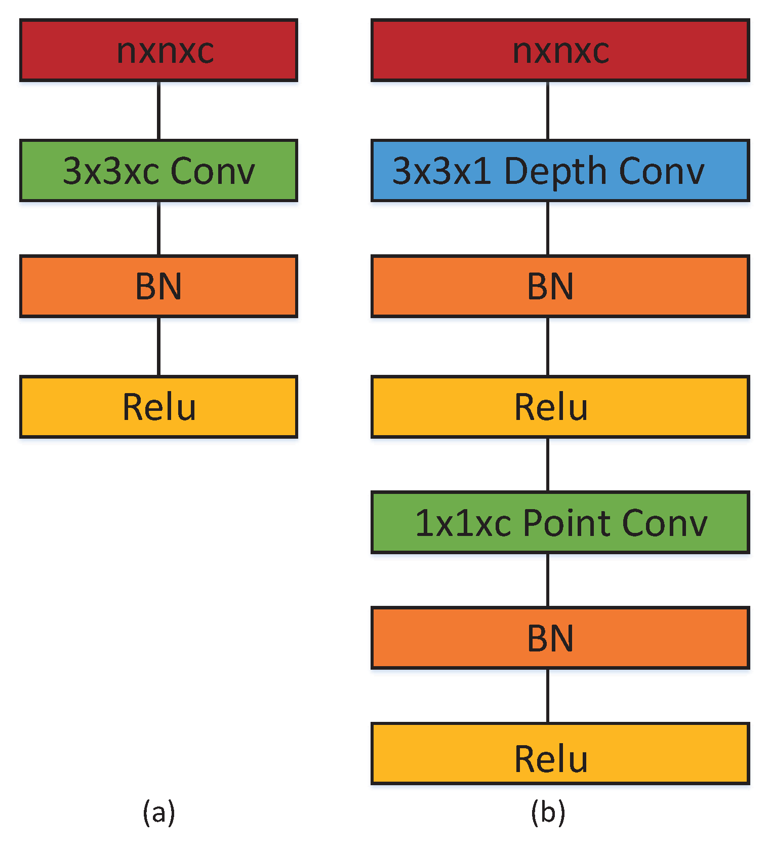
Because the classical SegNet uses a lot of convolution kernels, it generates a large number of parameters, making the model difficult to train and converge. In this paper, two improved networks are proposed. For the convolution layer, we use depthwise separable convolutions instead of standard convolutions, which greatly decreases the parameter numbers, shortens the training time, and makes the model easier to converge. Besides, the information loss caused by using this technique is at an acceptable level. In the experiment, the parameter numbers of SR-SegNet v1 is decreased by 71% and its training time is reduced by 18.3%. To compensate for the information loss caused by the usage of depthwise separable convolutions, we introduce dilated convolutions into the modified residual block and propose SR-SegNet v2. SR-SegNet v2’s parameter number is slightly increased compared with SR-SegNet v1, and its training time is reduced by 7.7% compared with the classical SegNet.

To compare the performance of each model, we tested every model under the same conditions. Table 3 shows the segmentation metrics of each model on the testing set. It can be seen that the metrics of SegNet are superior to those of FCN and DeconvNet. Compared with FCN8s, SegNet’s Ac, Dice, F1 and Miou are 4.88%, 17.2%, 7.83%, and 1.32% higher, respectively. Compared to the classical SegNet, SR-SegNet v2 yields a higher F1 by 0.1% (0.9949 vs. 0.9939), a higher Dice by 1.2% (0.9437 vs. 0.9317), and a higher Miou by 2.37% (0.9322 vs. 0.9085).

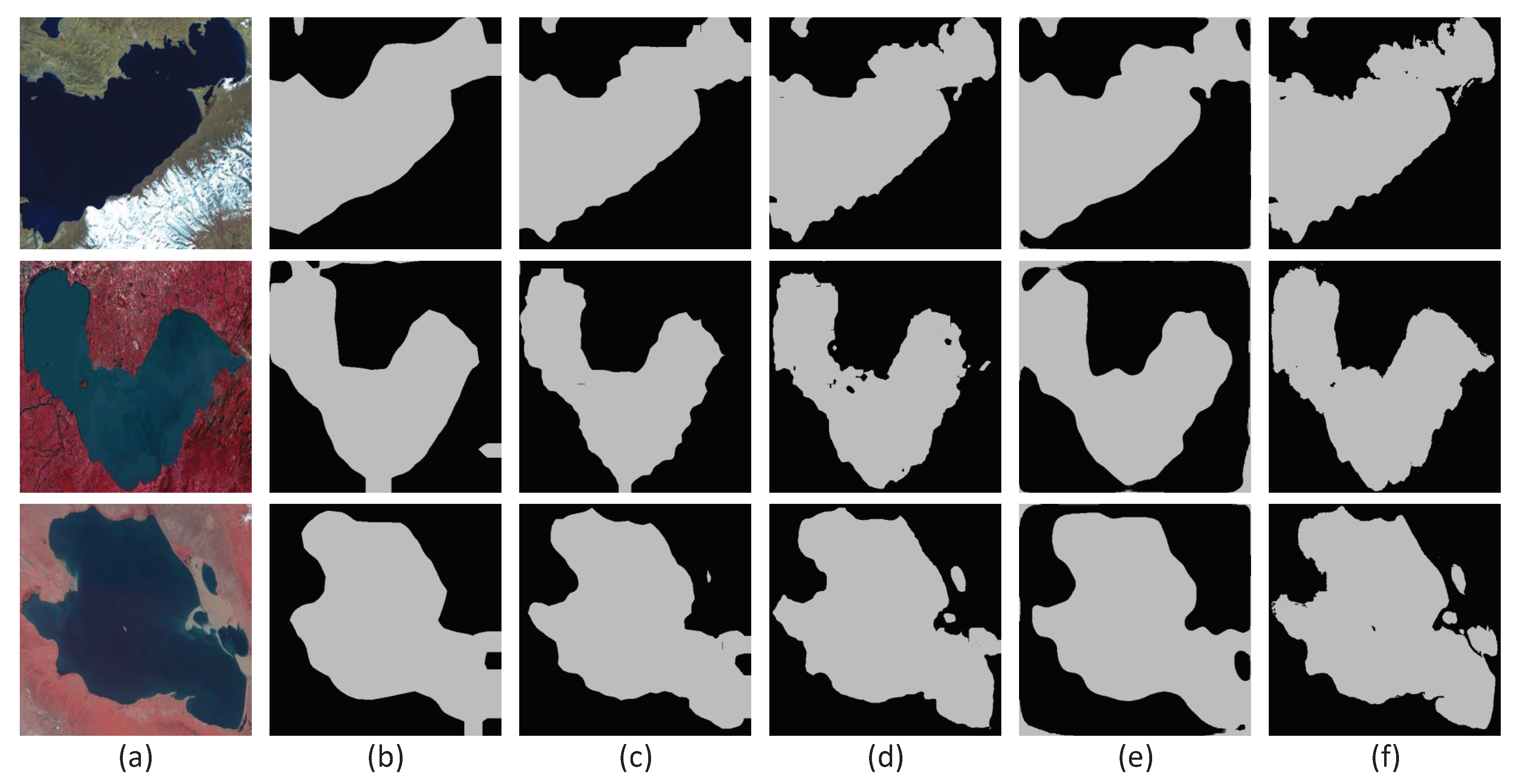
To further demonstrate the generalization performance of the network, the network trained using the Namsto Lake dataset was used to identify other lakes. In Figure 8, the first row is Namtso Lake, the second row is Chaohu Lake, and the third row is Qinghai Lake. It can be seen in Figure 8 that FCN and DeconvNet both adopt a simple encoding–decoding structure, and thus they could only identify the edge of the target very generally. The image spatial information is ignored in the extraction by FCN and DeconvNet, and thus neither extraction of lake boundary is fine enough. SR-SegNet can extract the lake location and boundary information better. In Figure 8f, it can be seen that SegNet has a better segmentation ability for all three lakes, but the details of the lakes are not extracted correctly, and the non-lake parts of Chaohu Lake are misidentified. Note that SR-SegNet can effectively solve the problem of network degradation and small lake recognition.

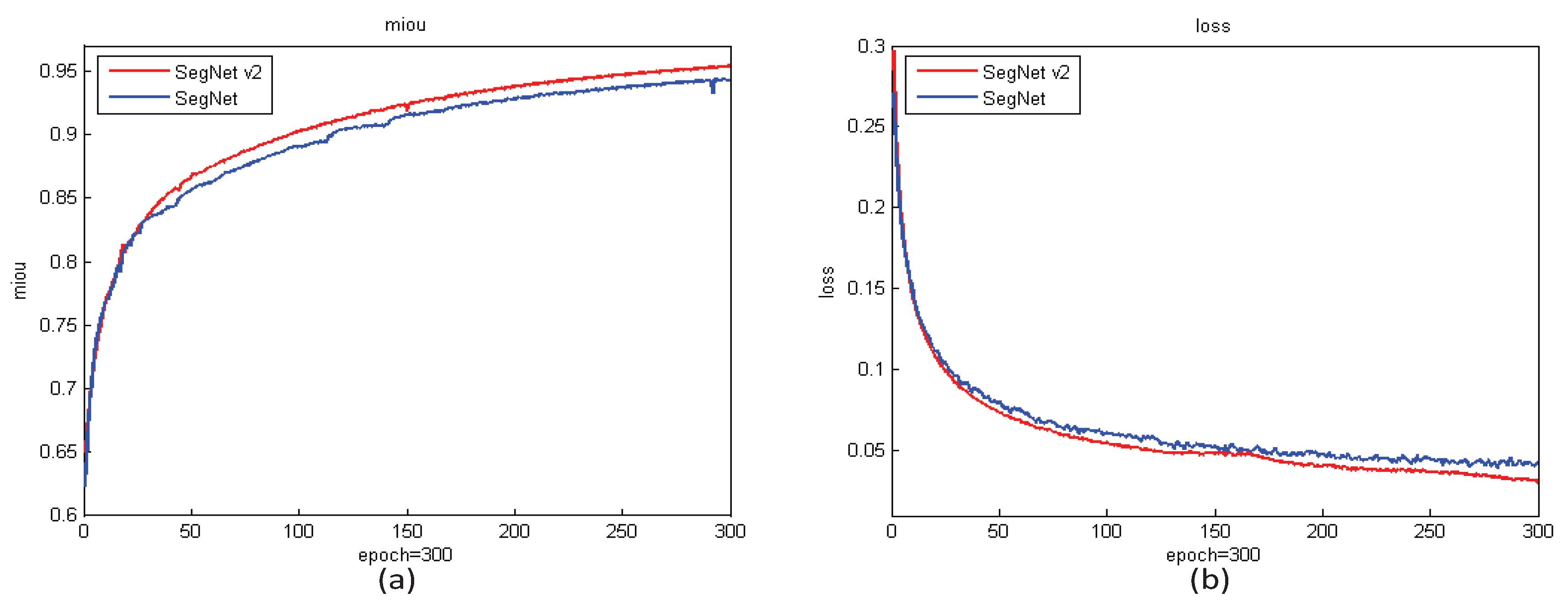
Figure 9 shows the training curves of SR-SegNet v2 and SegNet. It can be seen that SR-SegNet v2 performs better than SegNet, and its training process is smoother, whereas SegNet has many fluctuations. It is shown that the performance of the model is further improved with modified residual blocks added.

To demonstrate the superiority of the networks proposed in this paper, SegNet, SR-SegNet v1, and SR-SegNet v2 were tested and evaluated, respectively. Note that the proportion of lakes in a remote sensing image is relatively large, and the proportion of rivers in a remote sensing image is relatively small. Remote sensing images of lakes and rivers with both more positive pixels and fewer positive pixels were analyzed, respectively, in the experiment.

Table 4. Comparison of positive and negative pixels of test images. Positive Pixels, water body; Negative Pixels, non-water body; Proportion, the ratio of the number of positive pixels to the total pixels.

	Positive Pixels	Negative Pixels	Proportion (%)
Namtso Lake	120,103	142,041	45.82
Chaohu Lake	109,840	152,304	41.90
Qinghai Lake	142,718	119,426	54.44
River 1	17,768	244,376	6.78
River 2	20,206	241,938	7.71
River 3	13,677	248,467	5.22

shows the number of positive pixels (water body) and negative pixels (background) of six remote sensing images selected from the test images. The proportion represents the ratio of the number of positive pixels to total pixels. It can be seen that in a $512\times 512$ pixel remote sensing image, the number of lake pixels is 6 to 10 times greater than those of rivers.

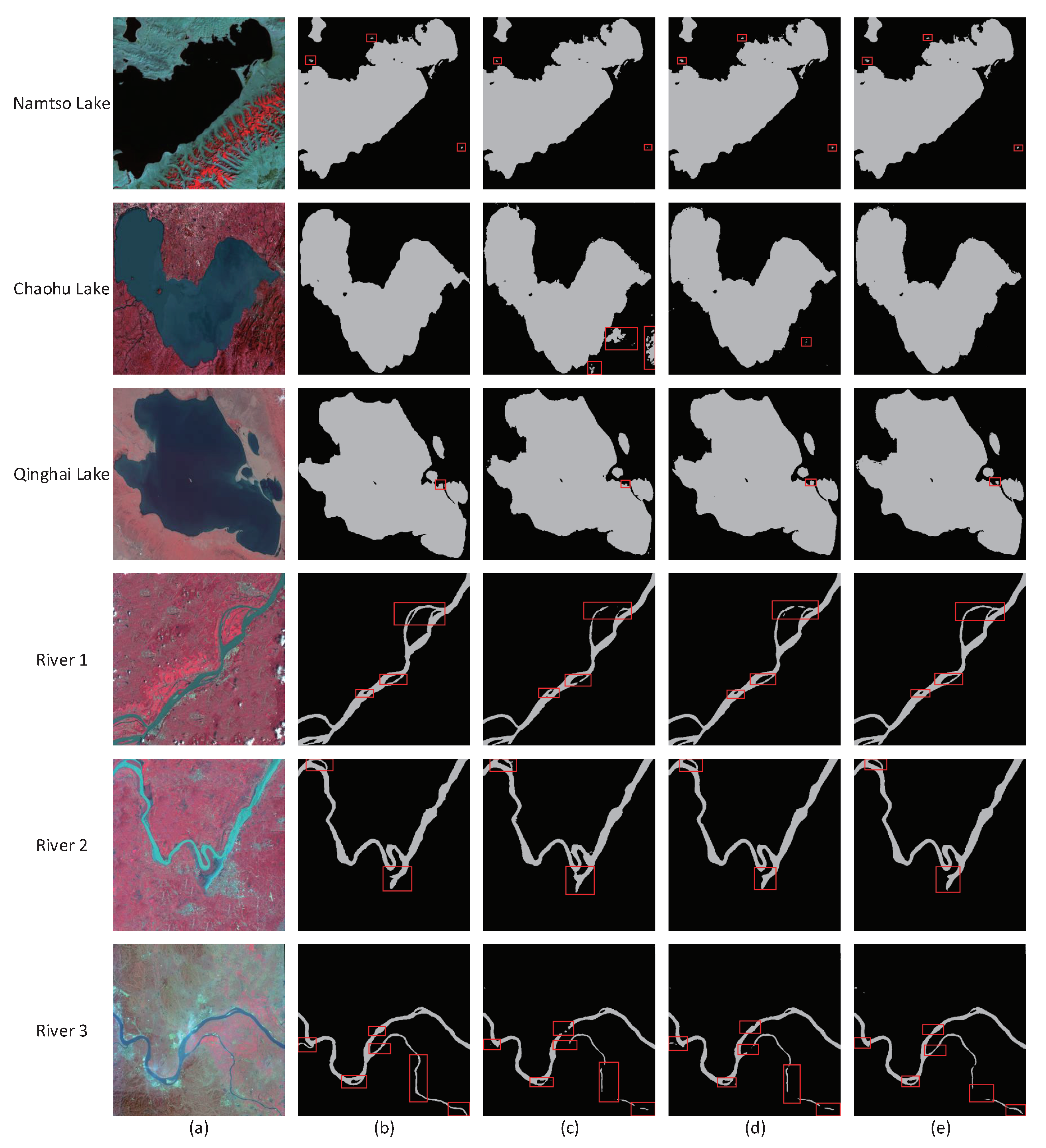
The segmentation results of test picture are shown in Figure 10. It can be seen that SegNet has a good segmentation ability for remote sensing images of lakes with more positive pixels. However, in the first row, the “small lake” near Namtso Lake is not recognized, proving that SegNet’s detection ability of small targets is poor. In contrast, SR-SegNet v2 solves this problem, with dilated convolutions in its modified residual blocks. This modification ensures the network’s better performance and increases the receptive field of the convolution layer. In the second row, SegNet dose not do well in Chaohu Lake’s segmentation, and there are many noises around the lake. However, the two improved networks proposed in this paper avoid degradation during training process and greatly reduce the noises, as a result of the introduction of modified residual blocks. The third row is the segmentation of Qinghai Lake; the extraction of lake boundary is not fine enough, which is also a problem to be solved in the future. It is worth noting that remote sensing images of Namtso Lake were used in training in this experiment, and remote sensing images of Qinghai Lake and Chaohu Lake were not included in the training set. However, good segmentation results for Qinghai lake and Chaohu Lake are given by SR-SegNet, which clearly proves the generalization abilities of the proposed networks.

In the experiments, it was found that river segmentation of SegNet is not as good as for the lake. This phenomenon has the following two explanations: first, the proportion of positive pixels in a river image is far less than the proportion of negative pixels; and, second, the extraction of river features is more complex than that of lake features. The classical SegNet performance degrades because there are too many deep layers, and a large number of training parameter is not helpful in dealing with complex features such as those of rivers. SR-SegNet V1 and SR-SegNet v2 are proposed to reduce the upsampling time and the training parameter number by using depth separable convolutions. At the same time, to reduce the depth of the network without affecting feature extraction, the modified residual block is introduced into the encoding stage to alleviate the problem of network degradation and extract more information. As shown in Figure 10, SR-SegNet is more effective in river segmentation, its results are closer to the real labels, and it can extract complex features which SegNet cannot. SR-SegNet v2 adds dilated convolutions to its convolution layers to further increase its receptive field. In the segmentation of Rivers 1 and 3, SegNet doe not work well on small river detection, because it cannot extract enough spatial information. In contrast, with the introduction of modified residual blocks, our proposed method can effectively extract spatial information for small river identification. In Figure 10, SR-SegNet v2 is able to segment River 3. As its receptive field expands, SR-SegNet v2 has a better result on river reach segmentation, and the result fully proves the effectiveness of dilated convolutions.

The model-testing times are shown in

Table 5. Model-testing time. The highest value for the testing time is highlighted in bold.

	Namtso Lake	Chaohu Lake	Qinghai Lake	River 1	River 2	River 3	Average/s
SegNet	0.9986	0.9955	0.9963	1.3456	1.5014	1.5234	1.2268
SR-SegNet v1	0.8221	0.8345	0.8190	0.9854	0.9765	0.9345	0.8953
SR-SegNet v2	0.9982	0.8673	0.8900	1.2478	1.0656	1.5012	1.0950

. After introducing depthwise separable convolutions and the residual structure, the network is simplified. The average testing time of SR-SegNet v1 is 27% shorter than that of the classical SegNet. In SR-SegNet v2, with extra dilated convolutions, the network computation is increased. Therefore, its average testing speed is only about 10% faster than that of the classical SegNet.

The results of the quantitative comparison are summarized in

Table 6. Quantitative result of different methods including SegNet, SR-SegNet v1, and SR-SegNet v2 on the selected six test images. The highest values for the different metrics are highlighted in bold.

Ac/%
	Namtso Lake	Chaohu Lake	Qinghai Lake	Lake Average	River 1	River 2	River 3	River Average
SegNet	99.67	99.28	99.56	99.50	98.91	98.95	98.62	98.83
SR-SegNet v1	99.63	99.35	99.47	99.48	99.11	99.30	99.07	99.16
SR-SegNet v2	99.69	99.56	99.42	99.56	99.15	99.26	99.01	99.14
F1/%
	Namtso Lake	Chaohu Lake	Qinghai Lake	Lake Average	River 1	River 2	River 3	River Average
SegNet	99.23	98.14	98.56	98.64	99.22	99.33	99.33	99.29
SR-SegNet v1	99.34	98.34	99.01	98.90	99.52	99.45	99.51	99.49
SR-SegNet v2	99.28	99.04	98.23	98.85	99.55	99.39	99.48	99.47
Miou/%
	Namtso Lake	Chaohu Lake	Qinghai Lake	Lake Average	River 1	River 2	River 3	River Average
SegNet	94.23	94.44	95.03	94.57	91.46	93.16	87.34	90.65
SR-SegNet v1	95.12	94.23	95.02	94.79	93.06	95.53	90.54	93.04
SR-SegNet v2	95.23	94.40	95.13	94.92	93.50	95.06	90.77	93.11

. In experiments on three lakes, it can be seen that SR-SegNet does not greatly outperform the classical SegNet; it only shows a small improvement. SR-SegNet v2 has a 99.56% Ac and a 94.92% Miou in the lake extraction, 0.06% and 0.35% higher than those of the classical SegNet, respectively.

However, for an image with complex rivers, where the number of positive pixels is far fewer than the number of negative pixels, the Ac and F1 of these three networks are relatively high, because there are fewer categories to classify, and the proportion of negative pixels in each image is very high. The selected Miou can distinguish all three networks more accurately. For Miou, SR-SegNet v2 hits the highest score with a gain of 2.46% compared to the classical SegNet (0.9311 vs. 0.9065) and SR-SegNet v1 achieves an improvement of 2.39% over the classical SegNet (0.9304 vs. 0.9065). The superiority of proposed networks in this paper for river extraction is thereby verified.

3.5. Verification Experiment

To further verify the generalization abilities of the models proposed in this paper, Cityscapes, a public dataset, was selected for further experiment. Due to the limitation of computer memory, this experiment did not use all categories of the Cityscapes dataset. Only four categories, namely human, car, road, and background, were selected. Then 2975 pictures were used as the training dataset and 2975 pictures as the validation dataset. With the Adam optimizer, the initial learning rate was 0.0001, the weight attenuation rate was 0.0005, the training batch batch-size was 3, and the iteration was 160 times.

The research topic of this paper is water area segmentation. To verify the generalization performance and effectiveness of the algorithms proposed in this paper, we selected a different dataset for verification. The biggest difference between the Cityscapes dataset and the water area segmentation dataset is that their objects are different, but using different objects for verification can better demonstrate the generalization performance of the networks proposed in this paper. The experimental results are shown in

Table 7. The results of validation dataset on the Cityscapes dataset. The highest value for the different metrics are highlighted in bold.

	Training Time/h	Miou/%
SegNet	23.25	81.24
SR-SegNet v2	21.32	82.25

. We can see that the training speed of V2 is increased by about 8.3%, and its Miou is also increased by 1.01%. Therefore, the generalization performance and effectiveness of the proposed network is verified.

4. Conclusions

In this paper, lake and river segmentation is improved by using SR-SegNet. Traditional decoding methods use 2× upsampling step by step, but this paper proposes to run 4× upsampling for the first time, and then removes three convolution layers with 512 channels each in decoding stage, thus reducing a large number of parameters and improving the training speed. At the same time, to extract more deep features and ensure the model’s segmentation accuracy, improved residual blocks are introduced into encoding stage to solve the problem of network degradation. Furthermore, to obtain a larger receptive field and obtain more spatial information, dilated convolutions are also added to convolution layers, and the cascading method is used to fuse the low-level and high-level features of the image.

The quantitative comparison results with SegNet, FCN, and DeconvNet demonstrates that SR-SegNet outperforms the other models. Compared with the standard SegNet, SR-SegNet gains a 2.37% improvements in Miou and saves 10–27% in model-testing time on the Lake and River dataset. However, due to the complexity of the model, this paper also needs to make improvements in the following aspects: (1) make the training process converge more quickly and improve the model’s training and prediction speed; (2) search more data and further improve the generalization performance of the model; and (3) solve the problem of small identification.

The data and the code of this study are available from the corresponding author upon request ([email protected]).

References

1. Wan, W.; Xiao, P.; Feng, X.; Li, H.; Ma, R.; Duan, H.; Zhao, L. Monitoring lake changes of Qinghai-Tibetan Plateau over the past 30 years using satellite remote sensing data. Chin. Sci. Bull. 2014, 59, 1021–1035. [Google Scholar] [CrossRef]
2. Gou, P.; Ye, Q.; Wei, Q. Lake ice change at the Nam Co Lake on the Tibetan Plateau during 2000–2013 and influencing factors. Prog. Geogr. 2015, 34, 1241–1249. [Google Scholar]
3. McFeeters, S. The use of the Normalized Difference Water Index (NDWI) in the delineation of open water features. Int. J. Remote Sens. 1996, 17, 1425–1432. [Google Scholar] [CrossRef]
4. Frazier, P.; Page, K. Water body detection and delineation with Landsat TM data. Photogramm. Eng. Remote Sens. 2000, 66, 1461–1467. [Google Scholar]
5. Yuan, X.; Sarma, V. Automatic urban water-body detection and segmentation from Sparse ALSM data via spatially constrained model-Driven clustering. IEEE Geosci. Remote Sens. Lett. 2011, 8, 73–77. [Google Scholar] [CrossRef]
6. Lu, S.; Wu, B.; Yan, N.; Wang, H. Water body mapping method with HJ-1A/B satellite imagery. Int. J. Appl. Earth Obs. Geoinf. 2011, 13, 428–434. [Google Scholar] [CrossRef]
7. Zhang, H.; Jiang, Q.; Xu, J. Coastline extraction using support vector machine from remote sensing image. J. Multimed. 2013, 8, 175–182. [Google Scholar]
8. Feyisa, G.; Meilby, H.; Fensholt, R.; Proud, S. Automated water extraction index: A new technique for surface water mapping using landsat image. Remote Sens. Environ. 2014, 140, 23–35. [Google Scholar] [CrossRef]
9. Michael, S.; Wei, L.; Zhu, X. Automatic coastline detection in non-locally filtered tandem-X data. In Proceedings of the 2015 IEEE International Geoscience and Remote Sensing Symposium (IGARSS), Milan, ltaly, 26–31 July 2015; pp. 1036–1039. [Google Scholar]
10. Du, Y.; Feng, G.; Li, Z.; Peng, X.; Ren, Z.; Zhu, J. A method for surface water body detection and dem generation with multigeometry TanDEM-X aata. IEEE J. Sel. Top. Appl. Earth Obs. Remote Sens. 2008, 12, 151–161. [Google Scholar] [CrossRef]
11. Park, C.; Jeon, J.; Moon, Y.; Eom, I. Single image based algal bloom detection using water areas segmentation and probabilistic algae indices. IEEE Geosci. Remote Sens. Lett. 2019, 7, 8869–8878. [Google Scholar]
12. Wang, B.; Wang, K.; Liao, W. Extraction of Qinghai-Tibet Plateau Lake based on remote sensing image segmentation. Remote Sens. Inf. 2018, 3, 117–122. [Google Scholar]
13. Cheng, B.; Cui, S.; Ma, X.; Liang, C. Research on an Urban Building Area Extraction Method with High-Resolution PolSAR Imaging Based on Adaptive Neighborhood Selection Neighborhoods for Preserving Embedding. ISPRS Int. J. Geo-Inf. 2020, 9, 109. [Google Scholar] [CrossRef] [Green Version]
14. Milosavljevic, A. Identification of Salt Deposits on Seismic Images Using Deep Learning Method for Semantic Segmentation. ISPRS Int. J. Geo-Inf. 2020, 9, 24. [Google Scholar] [CrossRef] [Green Version]
15. Simonyan, K.; Zisserman, A. Very deep convolutional networks for large-scale image recognition. arXiv 2014, arXiv:1409.155. [Google Scholar]
16. Szegedy, C.; Loffe, S.; Vanhoucke, V.; Alemi, A. Inception-v4,inception-resnet and the impact of residualconnections on learning. In Proceedings of the Thirty-first AAAI Conference on Artificial Intelligence, San Francisco, CA, USA, 4–9 February 2017. [Google Scholar]
17. Huang, G.; Liu, Z.; vander Maaten, L.; Weinberger, K.Q. Densely connected convolutional networks. In Proceedings of the IEEE Conference on Computer Vision and Pattern Recognition (CVPR), Honolulu, HI, USA, 21–26 July 2017. [Google Scholar]
18. Xia, M.; Li, Y.; Zhang, Y.; Weng, L.; Liu, J. Cloud/snow recognition of satellite cloud images based on multi-scale fusion attention network. J. Appl. Remote Sens. 2020, 14, 032609. [Google Scholar] [CrossRef]
19. Long, J.; Shelhamer, E.; Darrell, T. Fully convolutional networks for semantic segmentation. In Proceedings of the 2015 IEEE Conference on Computer Vision and Pattern Recognition (CVPR), Boston, MA, USA, 7–12 June 2015; pp. 3431–3440. [Google Scholar]
20. Noh, H.; Hong, S.; Han, B. Learning deconvolution network for semantic segmentation. arXiv 2015, arXiv:1505.04366. [Google Scholar]
21. Badrinarayanan, V.; Kendall, A.; Cipolla, R. SegNet: A deep convolutional encoder-decoder architecture for image segmentation. IEEE Trans. Pattern Anal. Mach. Intell. 2017, 39, 2481–2495. [Google Scholar] [CrossRef]
22. Zhao, H.; Shi, J.; Qi, X.; Wang, X.; Jia, J. Pyramid scene parsing network. In Proceedings of the 2017 IEEE Conference on Computer Vision and Pattern Recognition (CVPR), Honolulu, HI, USA, 21–26 July 2017; pp. 6230–6239. [Google Scholar]
23. Yu, F.; Koltun, V. Multi-Scale context aggregation by dilated convolution. In Proceedings of the International Conference on Learning Representations 2016 (ICLR), San Juan, Puerto Rico, 2–4 May 2016. [Google Scholar]
24. Xia, M.; Song, W.; Sun, X.; Liu, J.; Ye, T.; Xu, Y. Weighted Densely Connected Convolutional Networks for Reinforcement Learning. Int. J. Pattern Recognit. Artif. Intell. 2020, 34, 2052001. [Google Scholar] [CrossRef]
25. Chollet, F. Xception:Deep learning with depthwise separable Convolutions. In Proceedings of the 2017 IEEE Conference on Computer Vision and Pattern Recognition (CVPR). IEEE, Honolulu, HI, USA, 21–26 July 2017; pp. 1800–1807. [Google Scholar]
26. He, K.; Zhang, X.; Ren, S.; Sun, J. Deep residual learning for image recognition. In Proceedings of the 2016 IEEE Conference on Computer Vision and Pattern Recognition (CVPR), Las Vegas, NV, USA, 26 June–1 July 2016; pp. 770–778. [Google Scholar]
27. Xu, C. Research and Implementation of Neural Segmentation based on Deep Learning. Master’s Thesis, Bejing University of Posts and Telecommunications, Beijing, China, 2018. [Google Scholar]
28. Xia, M.; Liu, W.; Xu, Y.; Wang, K.; Zhang, X. Dilated Residual Attention Network for Load Disaggregation. Neural Comput. Appl. 2019, 31, 8931–8953. [Google Scholar] [CrossRef]
29. Liu, P.; Liu, X.; Liu, M.; Shi, Q.; Yang, J.; Xu, X.; Zhang, Y. Building footprint extraction from high-resolution images via spatial residual inception convolutional neural network. Remote Sens. 2019, 11, 830. [Google Scholar] [CrossRef] [Green Version]
30. Ioffe, S.; Szegedy, C. Batch normalization:accelerating deep network training by reducing internal covariate shift. In Proceedings of the 32nd International Conference on Machine Learning (ICML), Atlanta, GA, USA, 6–11 July 2015; pp. 448–456. [Google Scholar]
31. Krizhevsky, A.; Sutskever, I.; Hinton, G.E. Imagenet classification with deep convolutional neural network. In Proceedings of the Advances in Neural Information Processing Systems (NIPS), Lake Tahoe, ND, USA, 5–8 December 2015; pp. 1097–1105. [Google Scholar]
32. Sandler, M.; Howard, A.; Zhu, M.; Zhmoginov, A.; Chen, L. MobileNetV2: Inverted residuals and linear bottleneck. In Proceedings of the 2016 IEEE Conference on Computer Vision and Pattern Recognition (CVPR), Salt Lake City, UT, USA, 27–30 June 2016; pp. 4510–4520. [Google Scholar]
33. Pan, P.; Wang, Y.; Luo, Y.; Zhou, J. Automatic segmentation of nasopharyngeal neoplasm in MR image based on U-net model. J. Comput. Appl. 2019, 39, 1183–1188. [Google Scholar]
34. Ronneberger, O.; Fischer, P.; Brox, T. U-Net: Convolutional networks for biomedical image segmenation. In Proceedings of the 18th International Conference on Medical Image Computing and Computer Assisted lntervention (MICCAI), Munich, Germany, 5–9 October 2015; pp. 234–241. [Google Scholar]
35. Xia, M.; Qian, J.; Zhang, X.; Liu, J.; Xu, Y. River segmentation based on serparable attention residual network. J. Appl. Remote Sens. 2019, 14, 32602. [Google Scholar] [CrossRef]
36. Xia, M.; Zhang, X.; Liu, W.; Weng, L.; Xu, Y. Multi-stage Feature Constraints Learning for Age Estimation. IEEE Trans. Inf. Forensics Secur. 2020, 15, 2417–2428. [Google Scholar] [CrossRef]
37. Polak, M.; Zhang, H.; Pi, M. An evaluation metric for image segmentation of multiple objects. Image Vis. Comput. 2009, 27, 1223–1227. [Google Scholar] [CrossRef]
38. Bottou, L. Large-scale machine learning with stochastic gradient descent. In Proceedings of COMPSTAT; Springer: Berlin/Heidelberg, Germany, 2010; pp. 177–186. [Google Scholar]
39. Xia, M.; Zhang, C.; Wang, Y.; Liu, J.; Li, C. Memory based decision making: A spiking neural circuit model. Neural Netw. World 2019, 29, 135–149. [Google Scholar] [CrossRef] [Green Version]
40. LeCun, Y.; Boser, B.; Denker, J.; Henderson, D.; Jackel, L. Handwritten digit recognition with a back-propagation network. Adv. Neural Inf. Process. Syst. 1990, 396–404. [Google Scholar]
Figure 1. The structure of the proposed SR-SegNet.
Ijgi 09 00256 g001
Figure 2. Illustration of the residual block: (a) “bottleneck” shaped residual unit used in ResNet-50; and (b) the modified residual block of proposed in this paper. Dilated Conv, dilated convolution; Rate, dilation rate.
Ijgi 09 00256 g002
Figure 3. Standard convolution and dilated convolution: (a) standard convolution K = 3; (b) dilated convolution K = 3, rate = 2; and (c) dilated convolution K = 2, rate = 2.
Ijgi 09 00256 g003
Figure 4. Depthwise separable convolution for each input channel [29].
Ijgi 09 00256 g004
Figure 5. The details of standard convolution and depthwise separable convolution: (a) standard convolution; and (b) depthwise separable convolution. BN, batch normalization; Relu function, rectified linear unit.
Ijgi 09 00256 g005
Figure 6. Image and label example from the Lake and Rive dataset: (a) origin remote sensing images and their ground truth; and (b) data augment results of images and their ground truth.
Ijgi 09 00256 g006
Figure 7. The workflow of this study.
Ijgi 09 00256 g007
Figure 8. Test images, their predicted label images of compared five methods (gray: water body; black: background): (a) input image; (b) FCN32s; (c) FCN16s; (d) FCN8s; (e) DeconvNet; and (f) SR-SegNet v2. First row,: Namtso Lake; second row, Chaohu Lake; third row, Qinghai Lake.
Ijgi 09 00256 g008
Figure 9. Iteration plot on the Lake and Rive dataset of variations of the proposed methods: (a) plot of model Miou on the training dataset for SegNet and SR-SegNet v2; and (b) plot of model loss (cross-entropy) on the training dataset for SegNet and SR-SegNet v2.
Ijgi 09 00256 g009
Figure 10. Segmentation results of different methods on the Lake and River dataset (gray, water body; black, background): (a) input image; (b) ground truth; (c) SegNet; (d) SR-SegNet v1; and (e) SR-SegNet v2.
Ijgi 09 00256 g010