Applicability of a Recreational-Grade Interferometric Sonar for the Bathymetric Survey and Monitoring of the Drava River

 , ,
, ,  and
and 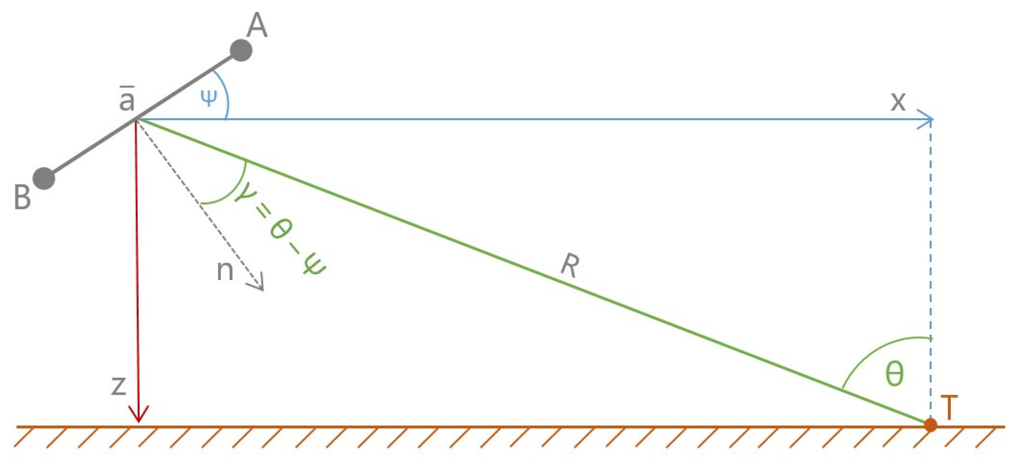
Abstract
1. Introduction
- Are these interferometric, recreational-grade sonars able to create a hydomorphologically correct, underwater elevation model of shallow lakes/rivers?
- Are these systems able to survey relatively large areas, like longer sections of a river?
- Does the application of interferometric recreational-grade fish-finder sonars have any advance over the classical cross-section or single-beam sonars?
- Is it feasible to build an efficient survey system based on interferometric fish-finders?
1.1. Evolution of Sonar Systems
- Single-beam sonars
- Multi-beam sonars
- Sidescan sonars, with to sub-groups:
- Traditional, symmetrical sidescan sonar for imaging purposes.
- Interferometric sonars, based on the measurement of phase difference; capable for wide-swath, 3D bathymetric measurements with wide aperture.
1.2. Interferometric Bathymetry Calculations in Recreational-Grade Sonar Systems
2. Materials and Methods
- Selecting the carrier platform, to minimize acoustic disturbances caused by the cavity and the boat engine; reduce the pitch, roll and heave movement of the hydrophones of the sonar.
- Selecting, then building an adequate sonar system, based on a recreational-grade sonar and its auxiliary devices and on a geodetic Global Navigation Satellite System (GNSS).
- Create a suspension to use the sonar securely. The suspension should resist collisions caused by the undetected floating objects and logs. In cases of emergency, the transducer should be removed from the water immediately.
- Processing of recreational-grade sonar output formats has never been common. To gain maximum control we developed our own sonar processing application.
- Create an effective measurement plan to maximize sounding quality.
- Bathymetry data alone is insufficient to characterize channel morphology: geodesic survey of the neighboring areas should be included, as well as the mapping artificial hydroengineering structures.
2.1. Carrier Platform
2.2. Sonar System and Auxiliary Devices
- The primary function was to establish a connection with the solid-state tri-axial gyroscope and magnetic compass (Lowrance® Precision–9, SW Ver.: 9.2; 1st row, 2nd column). With the readings of this gyroscope, the HDS module was able to counteract the vertical displacement of the interferometric bathymetry readings—even in case of extreme roll of the platform.
- This connector serves as the connection point of a submerged paddlewheel water speed and water temperature sensor. (Lowrance® EP–70R; 3rd row, on the right side).
- The tertiary function of NMEA 2000 is to connect a broadband radar device (not used in this research).
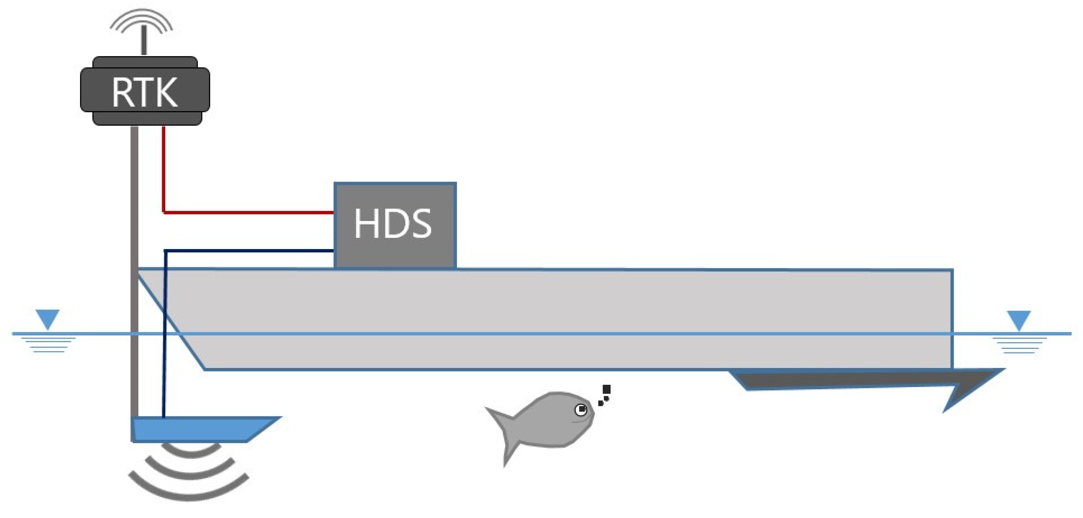
2.3. Setup of the Measurement System
2.4. Software Environment for Data Processing
- Open the SL3 files and restore the trajectory of the ship or boat; and overcome the limitation of Lowrance’s Mercator-like projection and restore the accuracy based on GNSS readings with the auxiliary “USR” files [32]. This trajectory includes millisecond level timestamp ‘X’ and ‘Y’ coordinates in a projected coordinate system, actual speed readings and actual heading (based on the trajectory of the GNSS and based on the solid state triaxial gyroscope (Lowrance®, Precision–9) to detect drift-like movements). The output point set is stored in File Geodatabase format, made by ESRI (Environmental System Research Institute, Redlands, CA, USA).
- Export sidescan imagery into perspective and georeferenced 8-bit Tagged Image File Format (TIFF) files, and export these readings into point cloud (File Geodatabase)
- Export single-beam and DownScan™ imagery into 8-bit TIFF files.
- Export 3D bathymetry readings into point cloud (File Geodatabase). This dataset is based on the processed interferometric measurements of the StructureScan 3D transducer.
- Filter erroneous readings, originated either from the GNSS or from the interferometric measurements.
2.5. Processing of the SL3 Files
- Conventional, downwards looking single-beam sonar datasets.
- Elliptic, high frequency, downwards looking single-beam sonar dataset.
- Sidescan datasets, to understand the morphology and textural pattern of the channel.
- Interferometric, 3-dimensional bathymetric packages for elevation data.
- We also identified two additional datasets. They are related to the raw data of the hydrophones and participating in the creation of 3D model, probably in such way, which is mentioned in [3].
- Millisecond-based timestamp.
- Speed over ground (measured in knots, based on the 10 Hz GNSS readings sent via NMEA 0183, floating point).
- Water speed (based on the readings of the paddlewheel sensor connected via NMEA 2000, floating point).
- The true heading (true course over ground) of the movement (based on GNSS readings, floating point).
- The magnetic heading (based on the magnetically referenced Lowrance® Precision–9).
- The elevation of the GNSS device, measured in feet over WGS84 (World Geodetic System 1984) ellipsoid (floating point).
- Position of the GNSS, recorded in integer numbers, projected to a metric grid (see below).
- Remove them completely, but in this case uncovered areas appear in the bathymetry.
- Correction with linear interpolation (or extrapolation at the extremities) based on their neighbors and assuming correct spatial data, hence the river surface is almost leveled, with minute downstream slope. Due to this procedure, several measurements are avoided, but likely, an error of 0.01–0.15 meters is introduced. In this case, the reduced precision in horizontal direction remains undetected and could cause a small ‘zigzag’ pattern in the final trajectory. The horizontal measurement errors usually appear jointly with the ‘height’ errors. However, after several trials, we found that these errors had a smaller effect on the final bathymetric product than the rejection of these points and exclusively relying on an interpolation algorithm.
2.6. Measurement Plan
2.7. Data Integration
- Single-part point data derived from the sonar readings. This is the major data source for riverbed interpolation. This dataset was stored in File Geodatabase. The Lowrance® sonars use a simplified horizontal reference system, called “Lowrance Mercator” which is based on a custom sphere. This reference system was transformed into EPSG 23700. The vertical reference system of the original sonar readings was based on the heights above the WGS84 geoid. These heights were then transformed into EPSG 5787 via the Lechner Knowledge Center’s transformation protocol.
- Contour lines of bank-full discharge. This dataset included the primary break lines for riverbed delineation. The 3D lines were transformed into high-density point datasets to avoid the “leaking” of the interpolation algorithm.
- Lines delineating the islands. Every island was delineated using the same steps mentioned above.
- LiDAR dataset of the research area. Every elevation reading comes from this LiDAR inside the islands and outside the banklines.
3. Results
- Trajectory of the boat in original, Lowrance Mercator projection, with 1-meter resolution and with restored precision (in separate feature classes). The route points were classified into primary (single-beam), DownScan™ (single-beam with narrow elliptic footprint, perpendicular to the trajectory), sidescan and interferometric 3D measurements. All route points possessed information on (1) measurement time (in UTC and in milliseconds since the beginning of the recording of the actual SL3 file); (2) flow velocity; (3) speed over ground (GNSS based); (4) the GNSS based heading; (5) magnetic heading (corrected by the declination); (6) water temperature; (7) the water depth under the transducer (measured by the single-beam sonar); (8) the minimum and maximum range of the sonar for the particular measurement type, based on the actual water depth; and (ix) a flag about the validity of the GNSS-supplied position. The ‘X’ and ‘Y’ coordinates were recorded in Lowrance Mercator; the ‘Z’ coordinate was recorded as the height over the WGS84 geoid. Every point was stamped with a record number for cross-processing with other datasets.
- Interferometric bathymetry measurements, in a multipoint feature class. This dataset contains cross-section-like bathymetric points perpendicular to the trajectory. Due to the limited accuracy of the sonar over a swath angle of 70° every point was rejected over this value automatically; so the effective aperture is 140° (theoretically, if the bottom is flat). Every measurement group was stored in one database row, with multiple points, and every point group is stamped with the record number (see above). The projection of the dataset is Lowrance Mercator. When our software calculates the coordinates of the points based on the ‘x’ and ‘z’ vectors (Figure 1), provided by the sonar, it takes the augmented trajectory line as primary coordinate. The ‘Z’ values of the points are bases on the GNSS height measured over the WGS84 geoid, and it was corrected by the length of the suspension rod. In this case the elevation information of the multipoints of the dataset are in absolute height values. This helps us to eliminate the issues caused by changing water level, and the changes in the draft caused by the different loads on the vessel. This was the primary dataset used for further processing.
- Sidescan measurements in a multipoint feature class. Due to the digital manner of the SL3 files, sidescan readings can be represented as individual points in 2D space. The structure of this dataset is similar to the interferometric measurements: the point of origin is positioned on the augmented trajectory line, but the displacement of the individual points is based on the range reported by the sonar. These points have no ‘Z’ information, hence they are positioned in the bottom of the channel, but the reflectance value is encoded as an ‘M’ property. This reflectance value is measured bytes, ranging from 0 to 255. Every cross-section-like point group has 3200 points based on the design of the SL3 file. These measurements are significantly distorted at their margins, closed to the river banks. The horizontal reference system is Lowrance Mercator.
- Geometrically corrected sidescan measurement in multipoint feature classes. This dataset has the same properties as the previously described one, but the points are corrected to the plane bottom, by simple Pythagorean theorem. The actual implementation for the sidescan sonar systems is described in [16]. In other software, able to export georeferenced, geometrically corrected sidescan images, the output is raster based. However, the distribution of the measured points does not correspond with a raster geometrically. Our primary idea was to use these points as an input of interpolation, to eliminate the distortions caused by the idea of the raster itself. Additional processing possibilities for this dataset are described in [41]. Similarly to [12,16], water column was removed in this dataset.
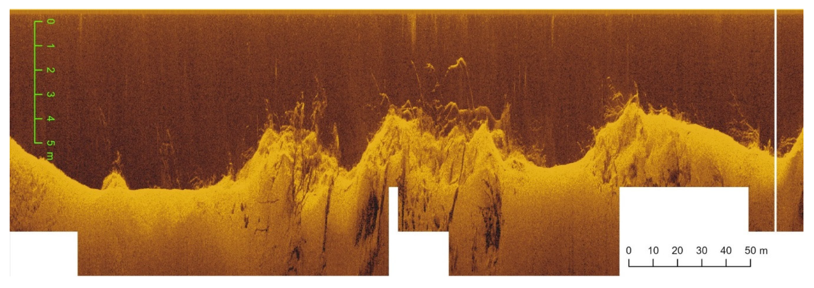
- In the first case, the images were exported in TIFF format, but no direct georeferencing information was included. The output images are horizontal and straight, in a consecutive order. During the survey, based on water depth, the range of the sonar is changing according to the inbuilt range categories of the Lowrance® unit. When sonar range altered a new image was started. In certain cases, the sonar omits some readings (it is likely caused by logs or other kind of floating objects or by serious turbulence). If the gap exceeded one meter, a new image was started to avoid the spread of the error over the whole image. Finally, a false georeferencing information was added to the images for visualization purposes: the images in this case were displayed in a straight manner, however the length along the trajectory line was accurate and the gaps are also displayed precisely. This false georeferencing helped to align different sonar products to each other than analyze them synoptically (usually sidescan and DownScan™). Compared to the length of an image the objects on the bottom usually look flat. To make the interpretation easier we added a transverse exaggeration of the factor of 10 through the false georeferencing. Every TIFF file was indexed on 8 bit, with a custom palette. As a last step, a Persistent Auxiliary Metadata dataset (PAM; *.tif.aux.xml) was added to the images to provide constant look through fixed statistics in different GDAL-based (Geospatial Data Abstraction Library) GIS applications (ArcGIS® Desktop and QGIS). A section of the river bottom is presented with false georeferencing in Figure 9 (DownScan™) and Figure 10 (sidescan).
- In the second case, the georeferenced images were exported in TIFF format (Figure 11). Georeferencing was implemented through the PAM dataset. In the case of sidescan three origin-destination control point pairs were added to the first column of the image: at top, left; left, at the middle; bottom left (always in pixel center). This pattern was repeated at least in the last column of the image or after every 25th column in the image. If the number of the control points on the given image was less than nine a standard polynomial adjustment was applied, otherwise spline was used. Some transverse exaggeration was also applied when the geometric correctness was not important in the actual situation. The ideal transverse exaggeration for sidescan imagery was 4.5.
- Output cell size: 1 m; snapped to a reference DEM (Digital Elevation Model) to prevent skidding between interpolation areas.
- Margin in cells: 5. This setting is used to prevent artifacts at the beginning and at the end of the river. On intermediate areas it is irrelevant.
- Drainage enforcement: “Do not enforce”. ANUDEM tries to create sink-free elevation models if no sink feature was provided. However, the underwater conditions do not correspond with land conditions, so the drainage enforcement should be avoided.
- Primary type of input data: “Spot”.
- Discretization error factor: 1.4. This slightly enhanced value is used to smooth smaller fluctuation.
- Vertical standard error: 0.1 m. In most cases, the pixels are oversampled by bathymetry data. This setting helps the ANUDEM to clean outliers in the group, caused by measurement error, or accidental events, like transiting logs in the water column.
- Tolerance №1: 0.3.
4. Discussion
5. Conclusions
Author Contributions
Funding
Acknowledgments
Conflicts of Interest
References
- Gips, B.; Williams, D.P. Through-the-sensor performance estimation of the Mondrian detection algorithm in sonar imagery. In Proceedings of the OCEANS 2018 MTS/IEEE Charleston, Charleston, SC, USA, 22–25 October 2018. [Google Scholar] [CrossRef]
- Williams, D. Cubist-Inspired Deep Learning with Sonar for UXO Detection and Classification; Final Report, USA Project MR18-1444; SERDP: Alexandria, VA, USA, 2019. [Google Scholar]
- Kuperman, W.; Roux, P. Underwater Acoustics. In Springer Handbook of Acoustics; Rossing, T., Ed.; Springer Science+Business Media: New York, NY, USA, 2007; p. 1286. [Google Scholar] [CrossRef]
- Gournia, C.; Fakiris, E.; Geraga, M.; Williams, D.P.; Papatheodorou, G. Automatic Detection of Trawl-Marks in Sidescan Sonar Images through Spatial Domain Filtering, Employing Haar-Like Features and Morphological Operations. Geosciences 2019, 9, 214. [Google Scholar] [CrossRef]
- Ferentinos, G.; Fakiris, E.; Christodoulou, D.; Geraga, M.; Dimas, X.; Georgiou, N.; Kordella, S.; Papatheodorou, G.; Prevenios, M.; Sotiropoulos, M. Optimal sidescan sonar and subbottom profiler surveying of ancient wrecks: The ‘Fiskardo’ wreck, Kefallinia Island, Ionian Sea. J. Archaeol. Sci. 2020, 113, 1–11. [Google Scholar] [CrossRef]
- Wada, M.; Yasui, S.; Saville, R.; Hatanaka, K. The development of a remote fish finder system for set-net fishery. In Proceedings of the 2014, Oceans—St. John’s, St. John’s, NL, Canada, 14–19 September 2014. [Google Scholar] [CrossRef]
- Kaeser, A.J.; Litts, T.L. An Illustrated Guide to Low-cost, Side Scan Sonar Habitat Mapping. Available online: https://www.fws.gov/panamacity/resources/An%20Illustrated%20Guide%20to%20Low-Cost%20Sonar%20Habitat%20Mapping%20v1.1.pdf (accessed on 28 January 2020).
- Kaeser, A.; Litts, T.; Tracy, T.W. Using Low-Cost Side-Scan Sonar for Benthic Mapping Throughout The Lower Flint River, Georgia, USA. River Res. Appl. 2012, 29, 634–644. [Google Scholar] [CrossRef]
- Shintaro, Y.; Toshitaka, K. A novel method of surveying submerged landslide ruins: Case study of the Nebukawa landslide in Japan. Eng. Geol. 2015, 186, 28–33. [Google Scholar] [CrossRef]
- Buscombe, D.; Grams, P.; Smith, S. Automated Riverbed Sediment Classification Using Low-Cost Sidescan Sonar. J. Hydraul. Eng. 2016, 142, 1–7. [Google Scholar] [CrossRef]
- Buscombe, D. Shallow water benthic imaging and substrate characterization using recreational-grade sidescan-sonar. Environ. Model. Softw. 2017, 89, 1–18. [Google Scholar] [CrossRef]
- Greene, A.; Rahman, A.; Kline, R.; Rahman, M.S. Side scan sonar: A cost-efficient alternative method for measuring seagrass cover in shallow environments. Estuar. Coast. Shelf Sci. 2018, 207, 250–258. [Google Scholar] [CrossRef]
- Ricart, A.M.; Sanmartí, N.; Pérez, M.; Romero, J. Multilevel assessments reveal spatially scaled landscape patterns driving coastal fish assemblages. Mar. Environ. Res. 2018, 140, 210–220. [Google Scholar] [CrossRef] [PubMed]
- Spirkovski, Z.; Ilik–Boeva, D.; Rittercusch, D.; Peveling, R.; Pietrock, M. Ghost net removal in ancient Lake Ohrid: A pilot study. Fish. Res. 2019, 211, 46–50. [Google Scholar] [CrossRef]
- Hook, J.D. Sturgeon Habitat Quantified by Side-Scan Sonar Imagery. Master of Science, University of Georgia, Athens, Georgia, USA. 2011. Available online: https://getd.libs.uga.edu/pdfs/hook_john_d_201105_ms.pdf (accessed on 28 January 2020).
- Blondel, P. The Handbook of Sidescan Sonar; Springer: Berlin/Heidelberg, Germany, 2009; p. 316. ISBN 978-3-642-43463-1. [Google Scholar] [CrossRef]
- Kirmani, S. Methods and Apparatuses for Reconstructing a 3d Sonar Image. U.S. Patent 2016/0259052 A1, 8 September 2016. [Google Scholar]
- Merklinger, H.; Ellis, D. Fessenden and Boyle: Two Canadian sonar pioneers. Proc. Meet. Acoust. 2017, 30, 1–20. [Google Scholar] [CrossRef]
- Medwin, H.; Clay, C. Fundamentals of Acoustical Oceanography; Academic Press: San Diego, CA, USA, 1998; ISBN 978-0-12-487570-8. [Google Scholar] [CrossRef]
- Lurton, X. Swath Bathymetry Using Phase Difference: Theoretical Analysis of Acoustical Measurement Precision. IEEE J. Ocean. Eng. 2000, 25, 351–363. [Google Scholar] [CrossRef]
- Proctor, A.L.; Parks, D.A.; Horner, R.J.; Hunt, M.D. System and Associated Methods for Updating Stored 3D Sonar Data. U.S. Patent 2016/0259050 A1, 8 September 2016. [Google Scholar]
- Grall, P.; Marszal, J. Investigation into interferometric sonar system accuracy. Hydroacoustics 2015, 18, 69–76. [Google Scholar]
- Ødegård, Ø.; Hansen, R.E.; Singh, H.; Maarleveld, T.J. Archaeological use of Synthetic Aperture Sonar on deepwater wreck sites in Skagerrak. J. Archaeol. Sci. 2018, 89, 1–13. [Google Scholar] [CrossRef]
- Empirical Bayesian Kriging (Geostatistical Analyst). Available online: https://pro.arcgis.com/en/pro-app/tool-reference/geostatistical-analyst/empirical-bayesian-kriging.htm (accessed on 28 January 2020).
- Schultz, J.J.; Healy, C.A.; Parker, K.; Lowers, B. Detecting submerged objects: The application of side scan sonar to forensic contexts. Forensic Sci. Int. 2013, 231, 306–316. [Google Scholar] [CrossRef] [PubMed]
- Coleman, A.R. Sonar Assembly for Reduced Interference. U.S. Patent 2013/0208568 A1, 15 August 2013. [Google Scholar]
- Proctor, A. Sonar System Using Frequency Bursts. U.S. Patent 2014/0010048 A1, 9 January 2014. [Google Scholar]
- StructureScan 3D Transducer Installation Manual. Available online: https://www.jgtech.com/pdf/SS3D-Transducer_IM_EN_988-10971-002_w.pdf (accessed on 28 January 2020).
- Grządziel, A.; Felski, A.; Wąż, M. Experience with the use of a rigidly-mounted side-scan sonar in a harbour basin bottom investigation. Ocean Eng. 2015, 109, 439–443. [Google Scholar] [CrossRef]
- 6205 Bathymetry & Side Scan System—User Hardware Manual (0014877_REV_F). Available online: https://www.edgetech.com/wp-content/uploads/2019/07/0014877_REV_F.pdf (accessed on 28 January 2020).
- Hansen, R. Introduction to Sonar. Available online: http://www.uio.no/studier/emner/matnat/ifi/INF-GEO4310/h12/undervisningsmateriale/sonar_introduction_2012_compressed.pdf (accessed on 28 January 2020).
- What Is GPSBabel? Available online: https://www.gpsbabel.org/people/index.html (accessed on 28 January 2020).
- Low2Ozi. Available online: http://sorvik.ru/zip/low2ozi.zip (accessed on 28 January 2020).
- Maître, H. Processing of Synthetic Aperture Radar Images; ISTE Ltd.: London, UK, 2008; p. 390. [Google Scholar] [CrossRef]
- SonarLogAPI. Available online: https://github.com/risty/SonarLogApi (accessed on 28 January 2020).
- node-sl2format. Available online: https://github.com/kmpm/node-sl2format (accessed on 28 January 2020).
- SL2. Available online: http://wiki.openstreetmap.org/wiki/SL2 (accessed on 28 January 2020).
- Halmai, Á.; Balatonyi, L.; Valkay, A.I.; Czigány, S.; Liptay, Z.Á.; Pirkhoffer, E. Új megközelítésű mederfelmérési technikák alkalmazása kisvízfolyásokon. Védelem Tudomány 2018, 4, 159–181. [Google Scholar]
- How Topo to Raster Works. Available online: http://pro.arcgis.com/en/pro-app/tool-reference/3d-analyst/how-topo-to-raster-works.htm (accessed on 28 January 2020).
- Lóczy, D. The Drava River: Environmental Problems and Solutions; Springer: Cham, Switzerland, 2018; p. 399. ISBN 978-3-319-92815-9. [Google Scholar] [CrossRef]
- Chang, Y.-C.; Hsu, S.-K.; Tsai, C.-H. Sidescan Sonar Image Processing: Correcting Brightness Variation and Patching Gaps. J. Mar. Sci. Technol. 2010, 18, 785–789. [Google Scholar]
- Arseni, M.; Voiculescu, M.; Georgescu, L.P.; Iticescu, C.; Rosu, A. Testing Different Interpolation Methods Based on Single Beam Echosounder River Surveying. Case Study: Siret River. ISPRS Int. J. Geo-Inf. 2019, 8, 507. [Google Scholar] [CrossRef]
- Salekin, S.; Burgess, J.H.; Morgenroth, J.; Mason, E.G.; Meason, D.F. A Comparative Study of Three Non-Geostatistical Methods for Optimising Digital Elevation Model Interpolation. ISPRS Int. J. Geo-Inf. 2018, 7, 300. [Google Scholar] [CrossRef]


© 2020 by the authors. Licensee MDPI, Basel, Switzerland. This article is an open access article distributed under the terms and conditions of the Creative Commons Attribution (CC BY) license (http://creativecommons.org/licenses/by/4.0/).
Share and Cite
Halmai, Á.; Gradwohl–Valkay, A.; Czigány, S.; Ficsor, J.; Liptay, Z.Á.; Kiss, K.; Lóczy, D.; Pirkhoffer, E. Applicability of a Recreational-Grade Interferometric Sonar for the Bathymetric Survey and Monitoring of the Drava River. ISPRS Int. J. Geo-Inf. 2020, 9, 149. https://doi.org/10.3390/ijgi9030149
Halmai Á, Gradwohl–Valkay A, Czigány S, Ficsor J, Liptay ZÁ, Kiss K, Lóczy D, Pirkhoffer E. Applicability of a Recreational-Grade Interferometric Sonar for the Bathymetric Survey and Monitoring of the Drava River. ISPRS International Journal of Geo-Information. 2020; 9(3):149. https://doi.org/10.3390/ijgi9030149
Chicago/Turabian StyleHalmai, Ákos, Alexandra Gradwohl–Valkay, Szabolcs Czigány, Johanna Ficsor, Zoltán Árpád Liptay, Kinga Kiss, Dénes Lóczy, and Ervin Pirkhoffer. 2020. "Applicability of a Recreational-Grade Interferometric Sonar for the Bathymetric Survey and Monitoring of the Drava River" ISPRS International Journal of Geo-Information 9, no. 3: 149. https://doi.org/10.3390/ijgi9030149
APA StyleHalmai, Á., Gradwohl–Valkay, A., Czigány, S., Ficsor, J., Liptay, Z. Á., Kiss, K., Lóczy, D., & Pirkhoffer, E. (2020). Applicability of a Recreational-Grade Interferometric Sonar for the Bathymetric Survey and Monitoring of the Drava River. ISPRS International Journal of Geo-Information, 9(3), 149. https://doi.org/10.3390/ijgi9030149