Multitemporal Land Use and Land Cover Classification from Time-Series Landsat Datasets Using Harmonic Analysis with a Minimum Spectral Distance Algorithm


Abstract
1. Introduction
2. Materials and Methods
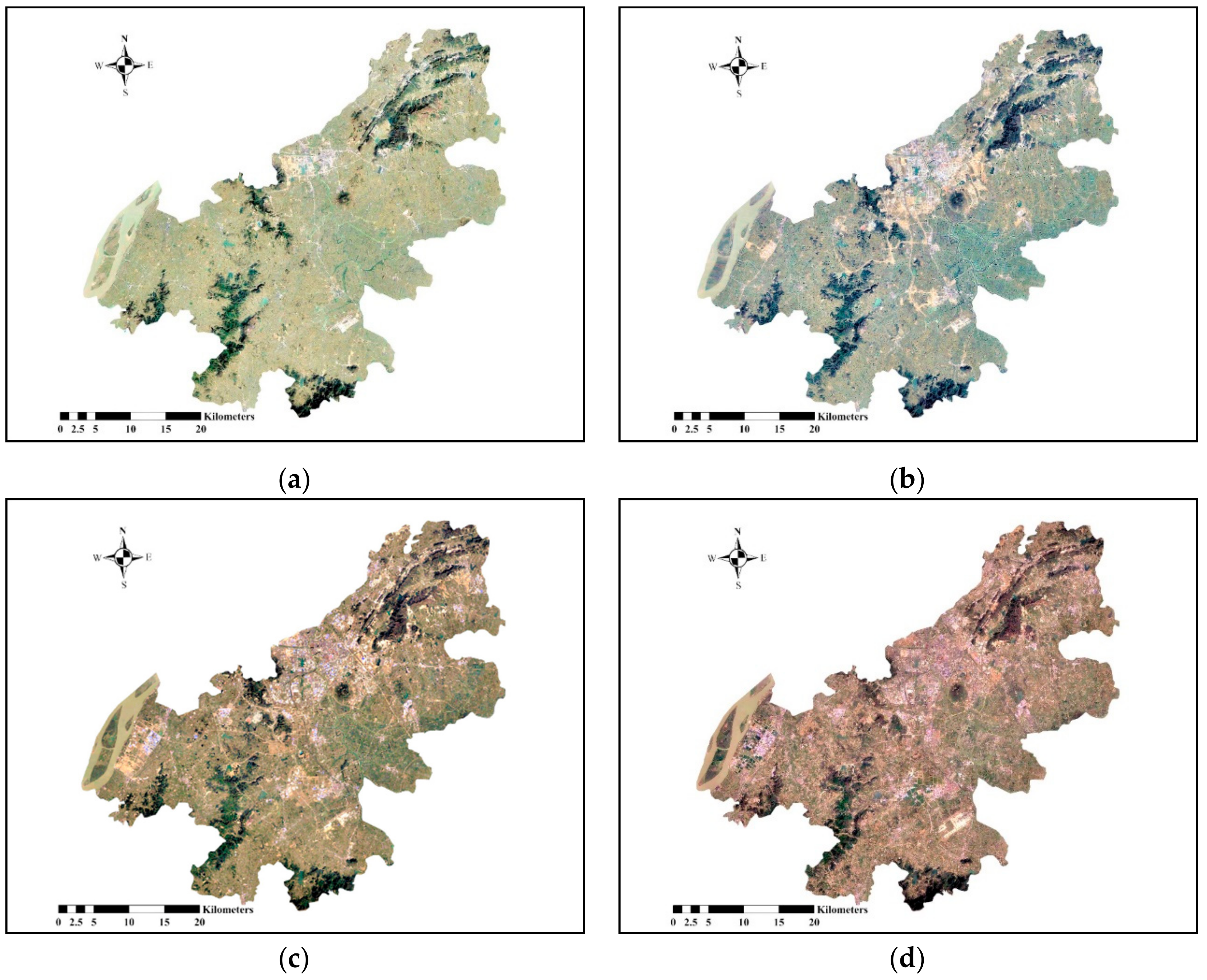
2.1. Study Area
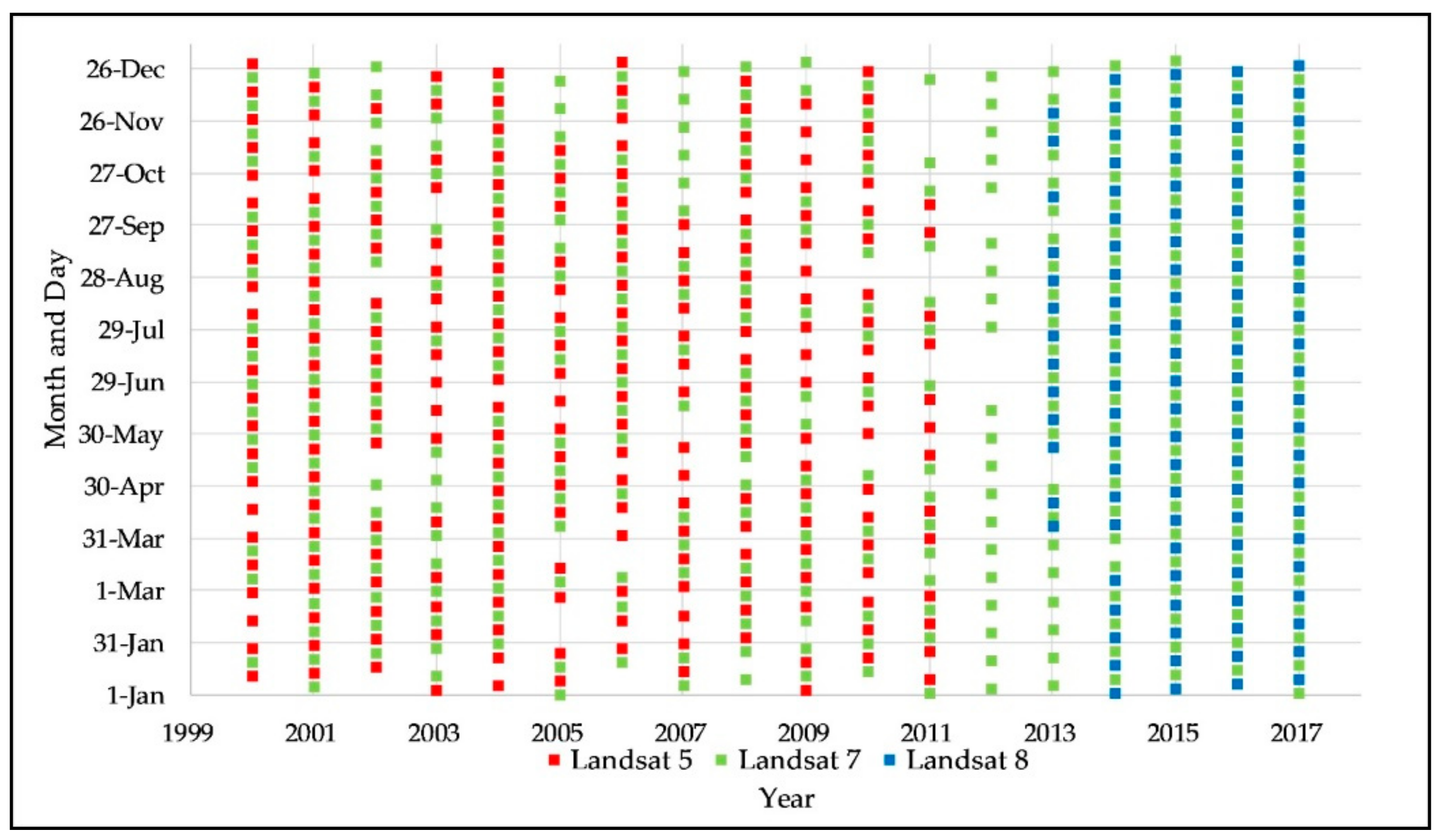
2.2. Datasets
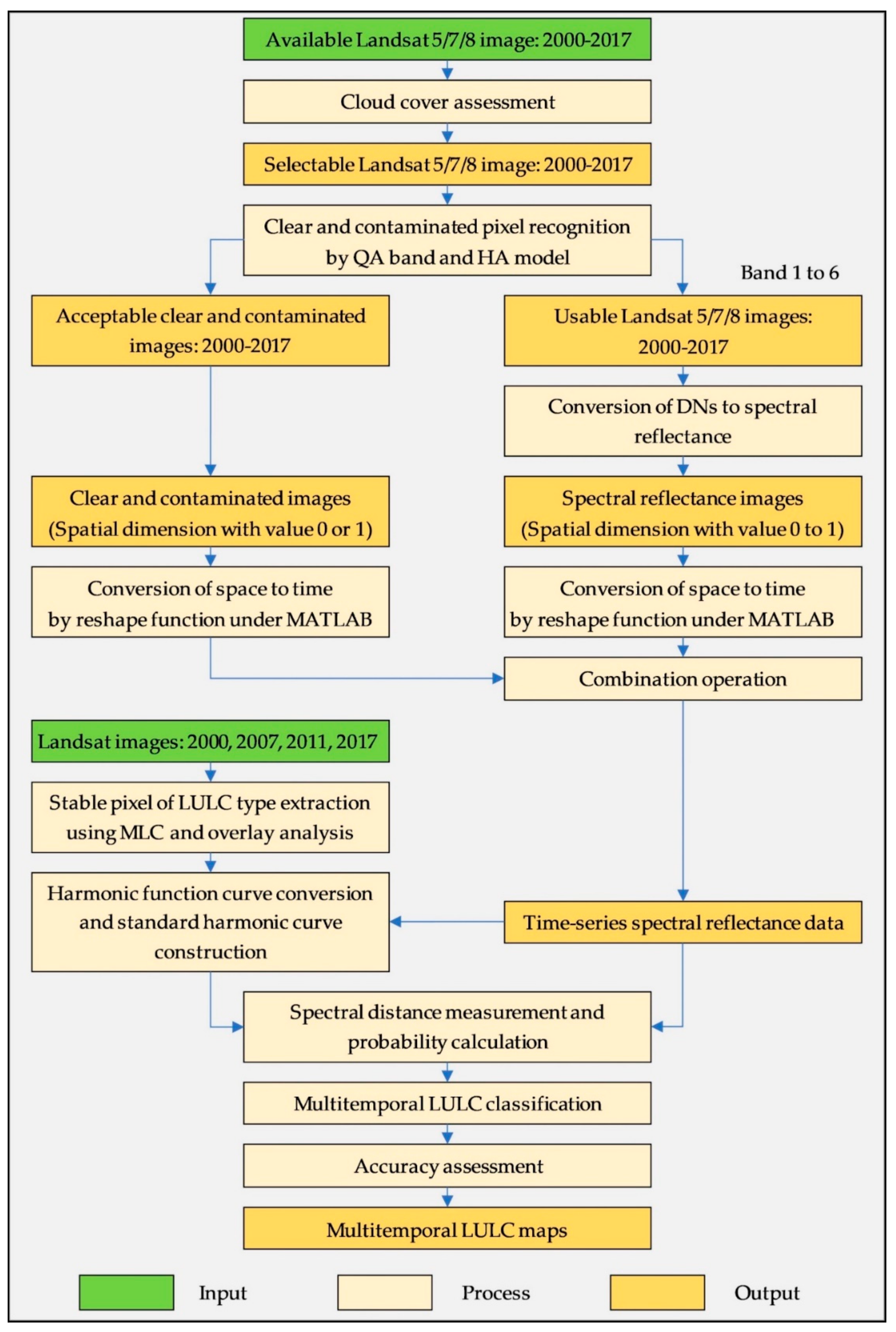
2.3. Research Methodology
2.3.1. Landsat Data Selection and Time-Series Spectral Reflectance Reconstruction
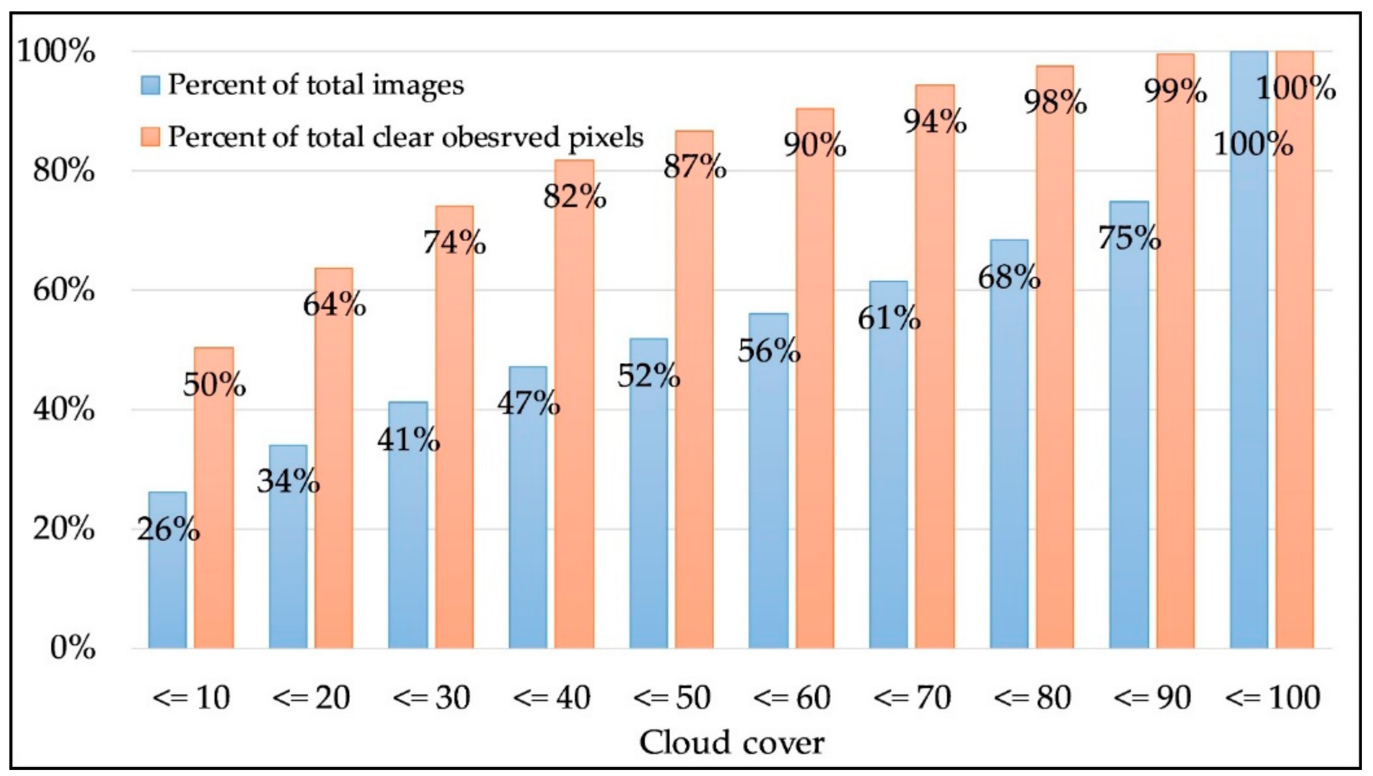
Cloud Cover Assessment
Clearly Observed and Contaminated Pixel Recognition
Conversion of Digital Numbers to Spectral Reflectance
Time-Series Spectral Reflectance Reconstruction
2.3.2. Multitemporal LULC Classification Using HA with the Minimum Spectral Distance Algorithm
Stable Pixels of the LULC Type Extraction
Harmonic Function Curve Transformation and Standard Harmonic Curve Construction
Spectral Distance Measurement and Probability Calculation
Multitemporal LULC Classification
Accuracy Assessment
3. Results
3.1. Selection of Landsat Data According to Cloud Cover Assessment
3.2. Reselection of Landsat Data Using the QA Band and HA Model
3.3. Spectral Reflectance Data
3.4. Time-Series Spectral Reflectance Reconstruction
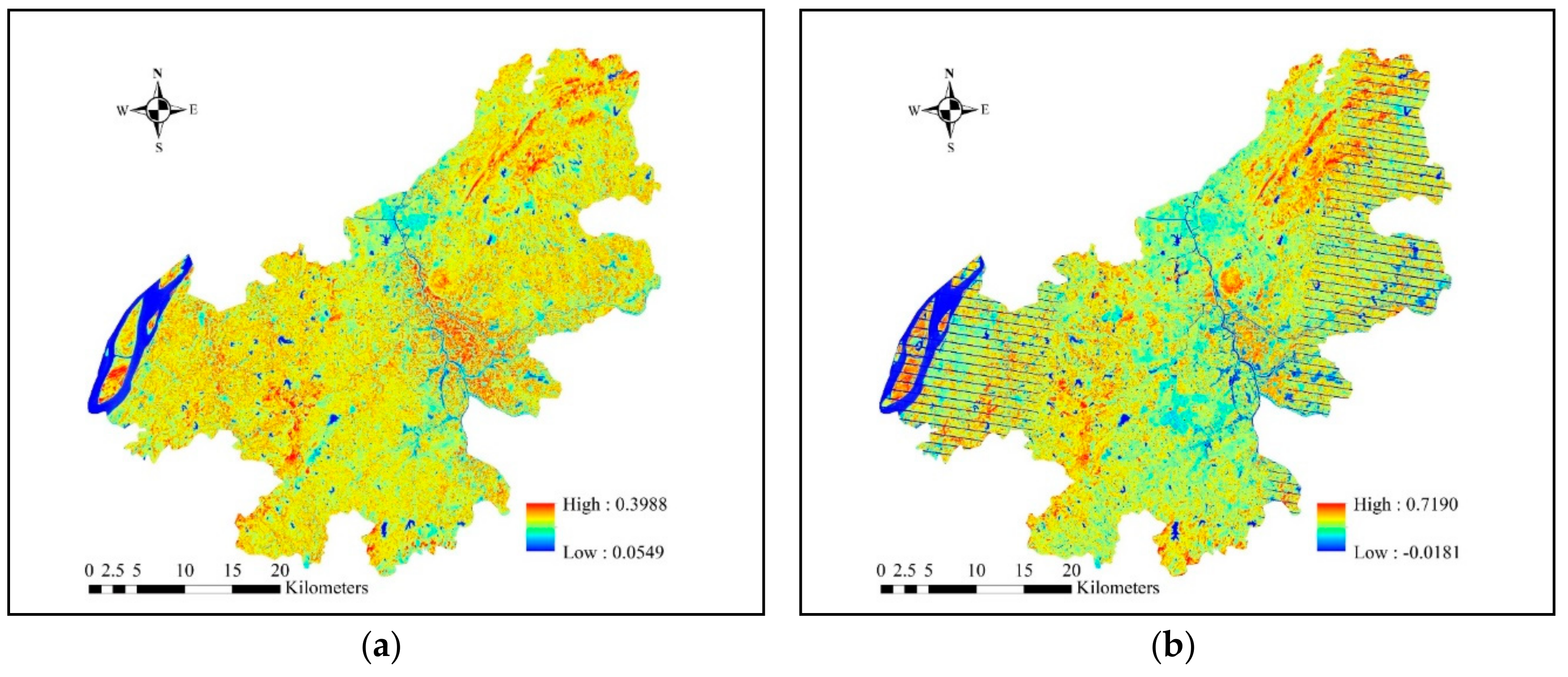
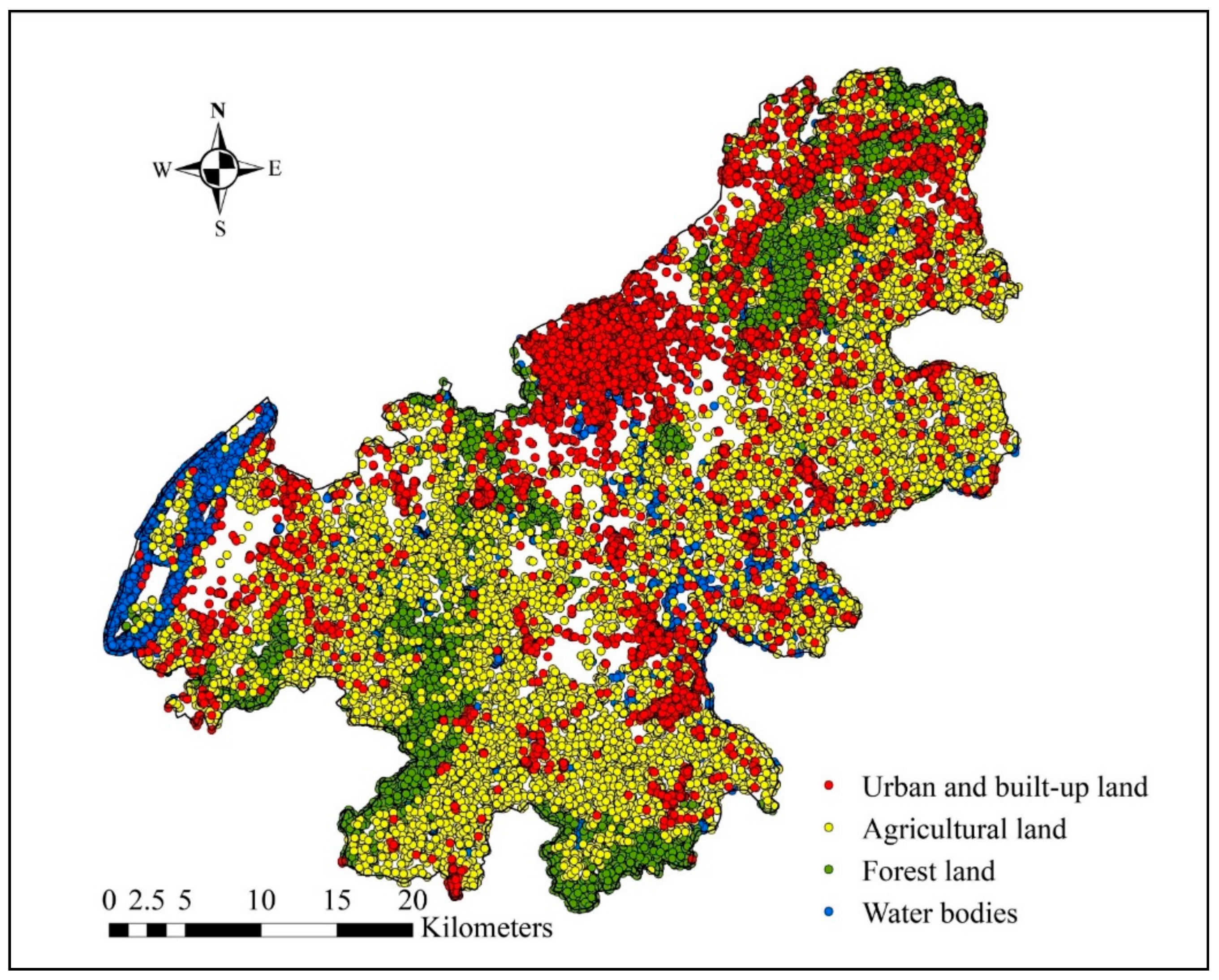
3.5. Stable Area of LULC Type Extraction
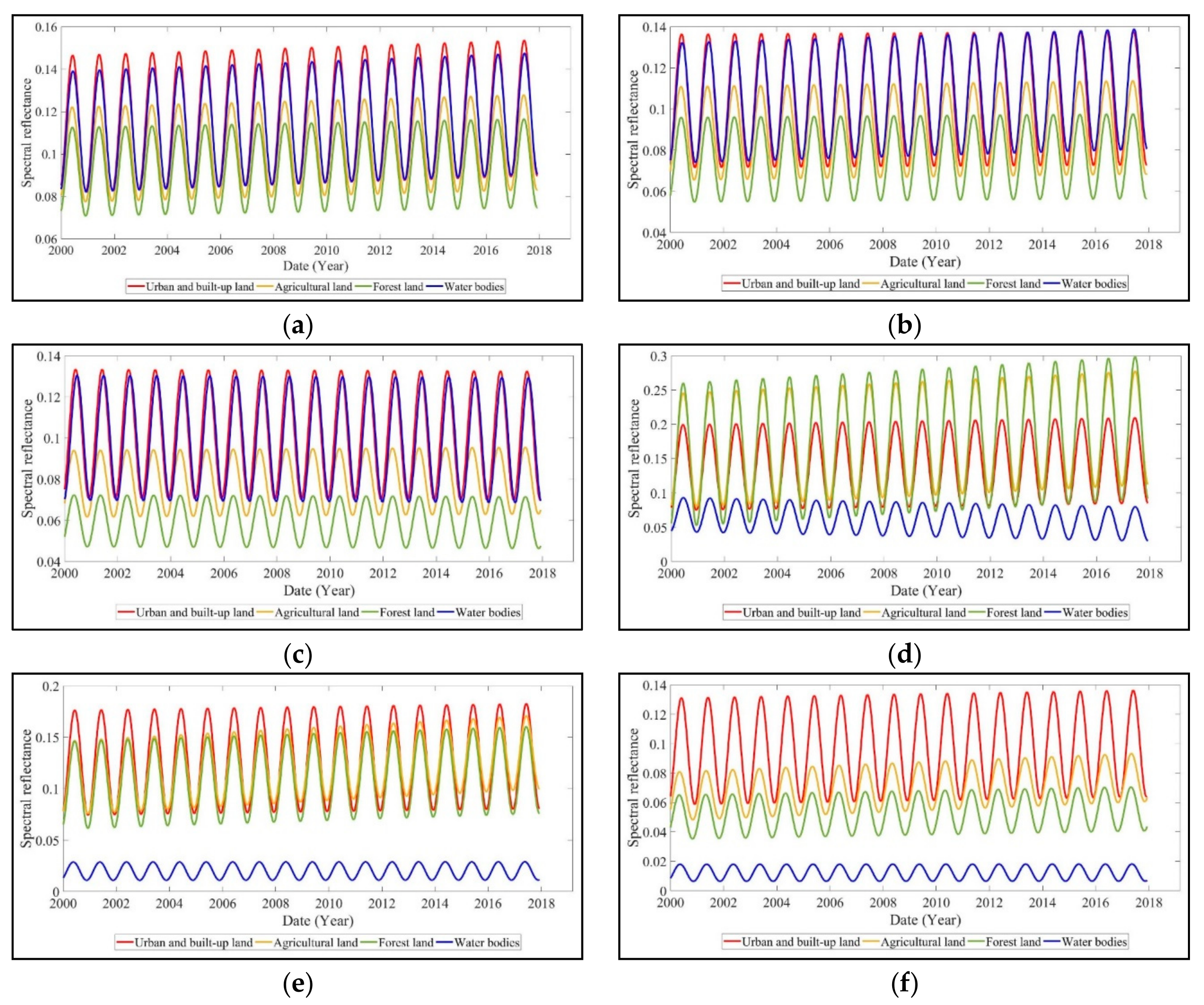
3.6. Spectral Harmonic Function Curve of LULC Types
3.7. Standard Harmonic Function Curve of Each LULC Type
3.8. Spectral Distance Measurement
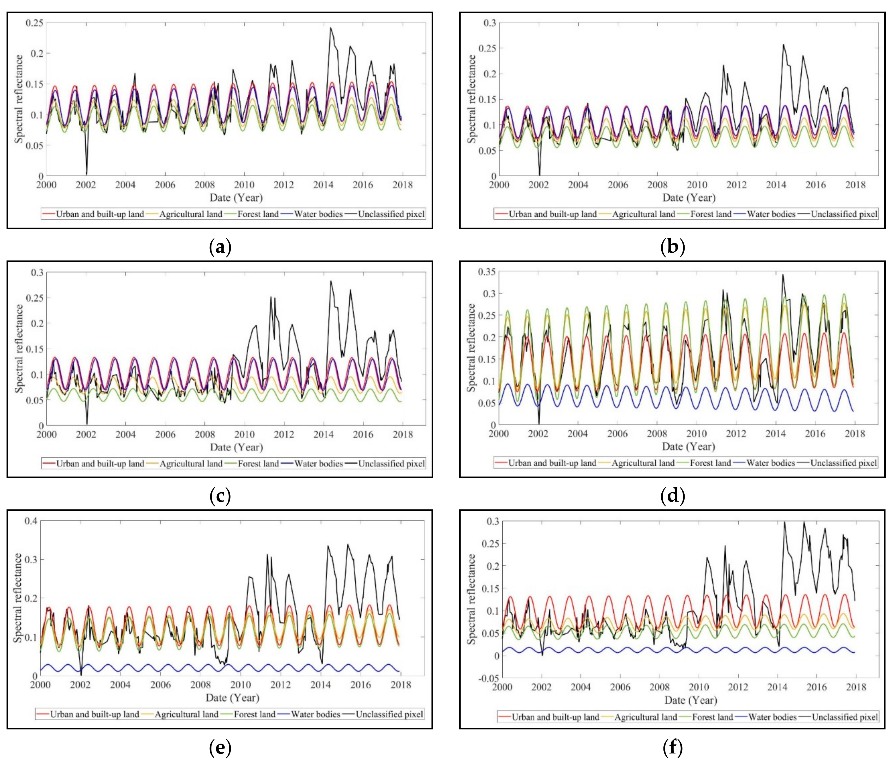
3.9. Probability of an Unclassified Pixel Being a Specific LULC Type
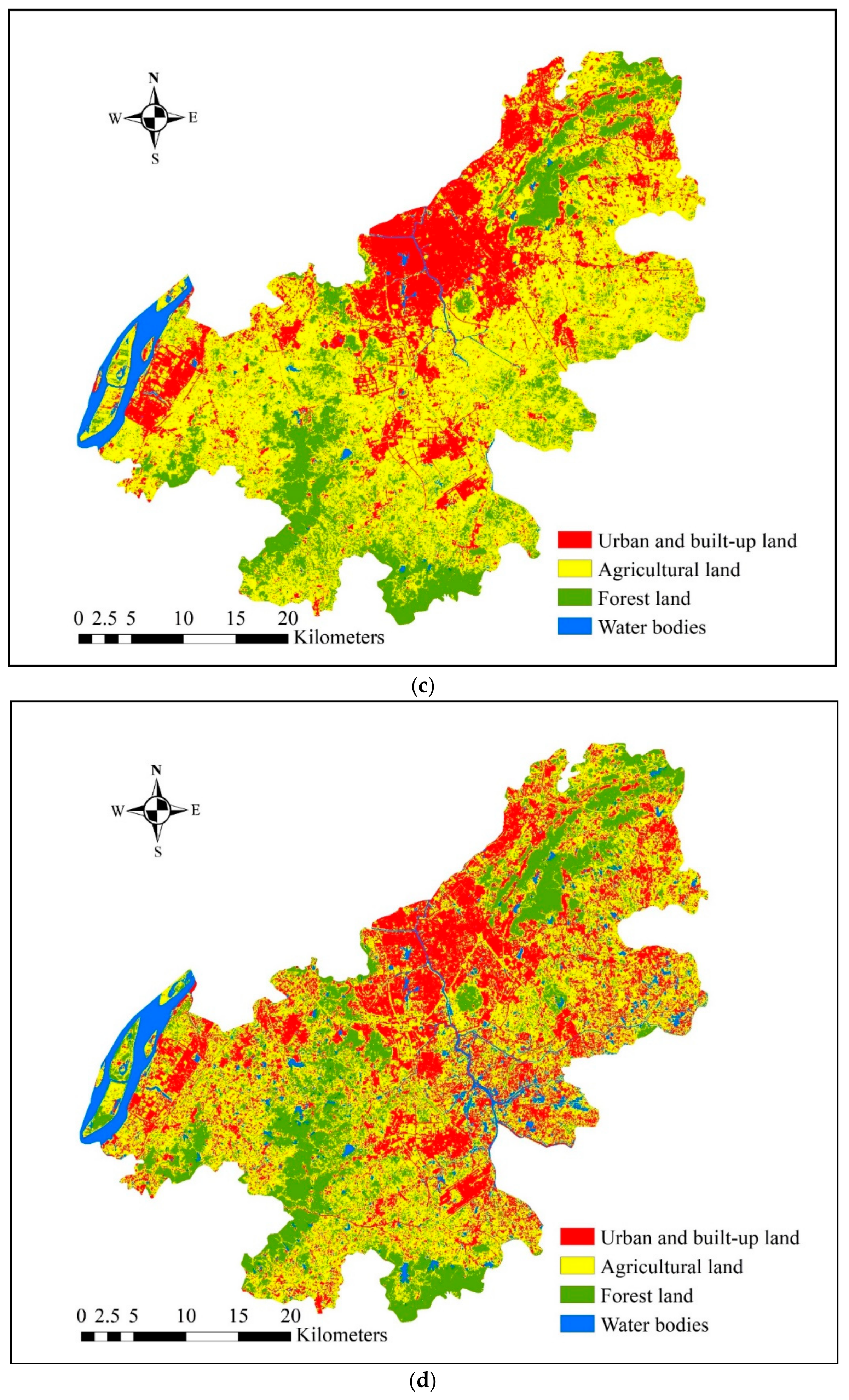
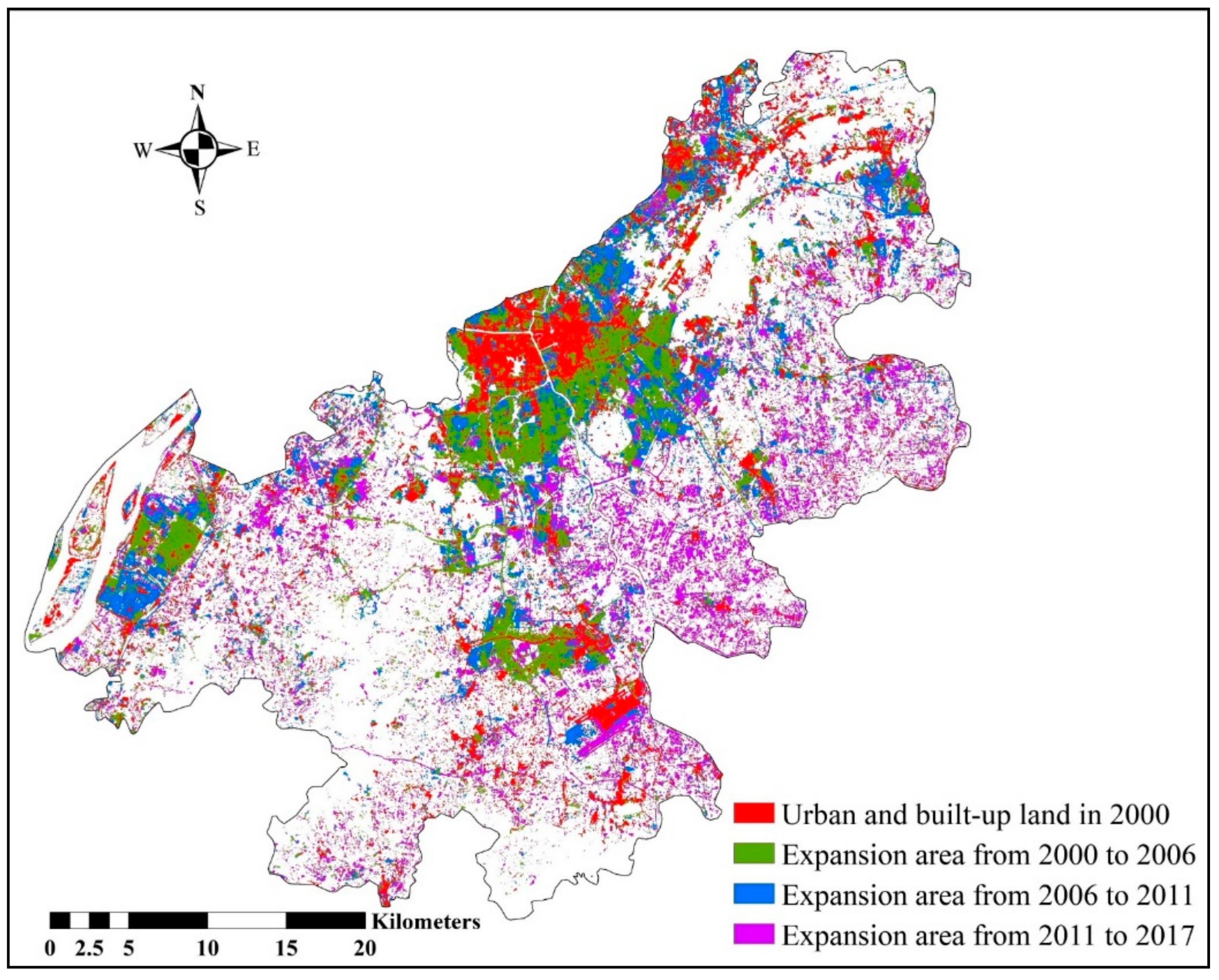
3.10. Multitemporal LULC Classification and Mapping
3.11. Accuracy Assessment of LULC Map
3.12. Accuracy Assessment of Change Detection
4. Discussion
4.1. Procedure for Landsat Image Selection
4.2. Semi-Automatic Time-Series Spectral Reflectance Reconstruction
4.3. Technique for the Extraction of a Stable Area for Each LULC Type
4.4. Supervised Classification Approach for Multitemporal LULC Mapping Using Harmonic Analysis with a Minimum Spectral Distance Algorithm
4.5. Accuracy Assessment of LULC Maps
5. Conclusions
Author Contributions
Funding
Acknowledgments
Conflicts of Interest
References
- Jensen, J.R. Introductory Digital Image Processing: A Remote Sensing Perspective; Prentice Hall Press: Upper Saddle River, NJ, USA, 2015; p. 544. [Google Scholar]
- Lo, C.P.; Quattrochi, D.A. Land Use and Land Cover Change, Urban Heat Island Phenomenon, and Health Implications: A Remote Sensing Approach. Photogramm. Eng. Remote Sens. 2003, 69, 1053–1063. [Google Scholar] [CrossRef]
- Warner, T.A.; Almutairi, A.; Lee, J.Y. Remote Sensing of Land Cover Change; SAGE Publications Ltd.: London, UK, 2009; p. 568. [Google Scholar]
- Weng, Q.; Fu, P.; Gao, F. Generating daily land surface temperature at Landsat resolution by fusing Landsat and MODIS data. Remote Sens. Environ. 2014, 145, 55–67. [Google Scholar] [CrossRef]
- Meyer, W.B.; Turner, B.L.I. Changes in Land Use and Land Cover: A Global Perspective; Cambridge University Press: Cambridge, UK, 1994; p. 537. [Google Scholar] [CrossRef]
- Al-shalabi, M.; Pradhan, B.; Billa, L.; Mansor, S.; Althuwaynee, O.F. Manifestation of Remote Sensing Data in Modeling Urban Sprawl Using the SLEUTH Model and Brute Force Calibration: A Case Study of Sana’a City, Yemen. J. Indian Soc. Remote Sens. 2013, 41, 405–416. [Google Scholar] [CrossRef]
- Fang, C.; Song, J.; Zhang, Q.; Li, M. The formation development and spatial heterogeneity patterns for the structures system of urban agglomerations in China. Acta Geogr. Sin. 2005, 60, 827–840. [Google Scholar]
- Turner, B.L.; Meyer, W.B.; Skole, D.L. Global Land-Use/Land-Cover Change: Towards an Integrated Study. Ambio 1994, 23, 91–95. [Google Scholar]
- Tolessa, T.; Senbeta, F.; Kidane, M. The impact of land use/land cover change on ecosystem services in the central highlands of Ethiopia. Ecosyst. Serv. 2017, 23, 47–54. [Google Scholar] [CrossRef]
- Seto, K.C.; Fragkias, M. Quantifying Spatiotemporal Patterns of Urban Land-use Change in Four Cities of China with Time Series Landscape Metrics. Landsc. Ecol. 2005, 20, 871–888. [Google Scholar] [CrossRef]
- Abdullah, A.Y.M.; Masrur, A.; Adnan, M.S.G.; Baky, M.A.A.; Hassan, Q.K.; Dewan, A. Spatio-Temporal Patterns of Land Use/Land Cover Change in the Heterogeneous Coastal Region of Bangladesh between 1990 and 2017. Remote Sens. 2019, 11, 790. [Google Scholar] [CrossRef]
- Fonseka, H.P.U.; Zhang, H.; Sun, Y.; Su, H.; Lin, H.; Lin, Y. Urbanization and Its Impacts on Land Surface Temperature in Colombo Metropolitan Area, Sri Lanka, from 1988 to 2016. Remote Sens. 2019, 11, 957. [Google Scholar] [CrossRef]
- Buitre, M.J.C.; Zhang, H.; Lin, H. The Mangrove Forests Change and Impacts from Tropical Cyclones in the Philippines Using Time Series Satellite Imagery. Remote Sens. 2019, 11, 688. [Google Scholar] [CrossRef]
- Mi, J.; Yang, Y.; Zhang, S.; An, S.; Hou, H.; Hua, Y.; Chen, F. Tracking the Land Use/Land Cover Change in an Area with Underground Mining and Reforestation via Continuous Landsat Classification. Remote Sens. 2019, 11, 1719. [Google Scholar] [CrossRef]
- Lu, D.; Li, L.; Li, G.; Fan, P.; Ouyang, Z.; Moran, E. Examining Spatial Patterns of Urban Distribution and Impacts of Physical Conditions on Urbanization in Coastal and Inland Metropoles. Remote Sens. 2018, 10, 1101. [Google Scholar] [CrossRef]
- Lacerda Silva, A.; Salas Alves, D.; Pinheiro Ferreira, M. Landsat-Based Land Use Change Assessment in the Brazilian Atlantic Forest: Forest Transition and Sugarcane Expansion. Remote Sens. 2018, 10, 996. [Google Scholar] [CrossRef]
- Mubako, S.; Belhaj, O.; Heyman, J.; Hargrove, W.; Reyes, C. Monitoring of Land Use/Land-Cover Changes in the Arid Transboundary Middle Rio Grande Basin Using Remote Sensing. Remote Sens. 2018, 10, 2005. [Google Scholar] [CrossRef]
- Gounaridis, D.; Symeonakis, E.; Chorianopoulos, I.; Koukoulas, S. Incorporating Density in Spatiotemporal Land Use/Cover Change Patterns: The Case of Attica, Greece. Remote Sens. 2018, 10, 1034. [Google Scholar] [CrossRef]
- Hurni, K.; Schneider, A.; Heinimann, A.; Nong, D.H.; Fox, J. Mapping the Expansion of Boom Crops in Mainland Southeast Asia Using Dense Time Stacks of Landsat Data. Remote Sens. 2017, 9, 320. [Google Scholar] [CrossRef]
- Wingate, V.R.; Phinn, S.R.; Kuhn, N.; Bloemertz, L.; Dhanjal-Adams, K.L. Mapping Decadal Land Cover Changes in the Woodlands of North Eastern Namibia from 1975 to 2014 Using the Landsat Satellite Archived Data. Remote Sens. 2016, 8, 681. [Google Scholar] [CrossRef]
- Alqurashi, A.F.; Kumar, L.; Sinha, P. Urban Land Cover Change Modelling Using Time-Series Satellite Images: A Case Study of Urban Growth in Five Cities of Saudi Arabia. Remote Sens. 2016, 8, 838. [Google Scholar] [CrossRef]
- Vittek, M.; Brink, A.; Donnay, F.; Simonetti, D.; Desclée, B. Land Cover Change Monitoring Using Landsat MSS/TM Satellite Image Data over West Africa between 1975 and 1990. Remote Sens. 2014, 6, 658–676. [Google Scholar] [CrossRef]
- Fu, P.; Weng, Q. A time series analysis of urbanization induced land use and land cover change and its impact on land surface temperature with Landsat imagery. Remote Sens. Environ. 2016, 175, 205–214. [Google Scholar] [CrossRef]
- Gillanders, S.N.; Coops, N.C.; Wulder, M.A.; Gergel, S.E.; Nelson, T. Multitemporal remote sensing of landscape dynamics and pattern change: Describing natural and anthropogenic trends. Prog. Phys. Geogr. Earth Environ. 2008, 32, 503–528. [Google Scholar] [CrossRef]
- Gómez, C.; White, J.C.; Wulder, M.A. Optical remotely sensed time series data for land cover classification: A review. ISPRS J. Photogramm. Remote Sens. 2016, 116, 55–72. [Google Scholar] [CrossRef]
- Gray, J.; Song, C. Consistent classification of image time series with automatic adaptive signature generalization. Remote Sens. Environ. 2013, 134, 333–341. [Google Scholar] [CrossRef]
- Song, C.; Woodcock, C.E.; Seto, K.C.; Lenney, M.P.; Macomber, S.A. Classification and Change Detection Using Landsat TM Data: When and How to Correct Atmospheric Effects? Remote Sens. Environ. 2001, 75, 230–244. [Google Scholar] [CrossRef]
- Liu, D.; Cai, S. A Spatial-Temporal Modeling Approach to Reconstructing Land-Cover Change Trajectories from Multi-temporal Satellite Imagery. Ann. Assoc. Am. Geogr. 2012, 102, 1329–1347. [Google Scholar] [CrossRef]
- Pouliot, D.; Latifovic, R.; Zabcic, N.; Guindon, L.; Olthof, I. Development and assessment of a 250m spatial resolution MODIS annual land cover time series (2000–2011) for the forest region of Canada derived from change-based updating. Remote Sens. Environ. 2014, 140, 731–743. [Google Scholar] [CrossRef]
- White, M.A.; de Beurs, K.M.; Didan, K.; Inouye, D.W.; Richardson, A.D.; Jensen, O.P.; O’Keefe, J.; Zhang, G.; Nemani, R.R.; van W.J.D., L.; et al. Intercomparison, interpretation, and assessment of spring phenology in North America estimated from remote sensing for 1982-2006. Glob. Chang. Biol. 2009, 15, 2335–2359. [Google Scholar] [CrossRef]
- Julien, Y.; Sobrino, J.A.; Verhoef, W. Changes in land surface temperatures and NDVI values over Europe between 1982 and 1999. Remote Sens. Environ. 2006, 103, 43–55. [Google Scholar] [CrossRef]
- Jakubauskas, M.E.; Legates, D.R.; Kastens, J.H. Crop identification using harmonic analysis of time-series AVHRR NDVI data. Comput. Electron. Agric. 2002, 37, 127–139. [Google Scholar] [CrossRef]
- Azzali, S.; Menenti, M. Mapping vegetation-soil-climate complexes in southern Africa using temporal Fourier analysis of NOAA-AVHRR NDVI data. Int. J. Remote Sens. 2000, 21, 973–996. [Google Scholar] [CrossRef]
- Menenti, M.; Azzali, S.; Verhoef, W.; van Swol, R. Mapping agroecological zones and time lag in vegetation growth by means of fourier analysis of time series of NDVI images. Adv. Space Res. 1993, 13, 233–237. [Google Scholar] [CrossRef]
- Keenan, T.F.; Gray, J.; Friedl, M.A.; Toomey, M.; Bohrer, G.; Hollinger, D.Y.; Munger, J.W.; O’Keefe, J.; Schmid, H.P.; Wing, I.S.; et al. Net carbon uptake has increased through warming-induced changes in temperate forest phenology. Nat. Clim. Chang. 2014, 4, 598. [Google Scholar] [CrossRef]
- Jia, L.; Shang, H.; Hu, G.; Menenti, M. Phenological response of vegetation to upstream river flow in the Heihe River basin by time series analysis of MODIS data. Hydrol. Earth Syst. Sci. 2011, 15, 1047–1064. [Google Scholar] [CrossRef]
- Wardlow, B.D.; Egbert, S.L.; Kastens, J.H. Analysis of time-series MODIS 250 m vegetation index data for crop classification in the U.S. Central Great Plains. Remote Sens. Environ. 2007, 108, 290–310. [Google Scholar] [CrossRef]
- Wardlow, B.D.; Egbert, S.L. Large-area crop mapping using time-series MODIS 250 m NDVI data: An assessment for the U.S. Central Great Plains. Remote Sens. Environ. 2008, 112, 1096–1116. [Google Scholar] [CrossRef]
- Thenkabail, P.S.; Schull, M.; Turral, H. Ganges and Indus river basin land use/land cover (LULC) and irrigated area mapping using continuous streams of MODIS data. Remote Sens. Environ. 2005, 95, 317–341. [Google Scholar] [CrossRef]
- Wit, A.D.; Su, B. Deriving phenological indicators from SPOT-VGT data using the HANTS algorithm. In 1998–2004: 6 Years of Operational Activities, Proceedings of the 2nd International VEGETATION User Conference, Antwerp, Belgium, 24–26 March; EC: Luxembourg, 2004; pp. 195–201. [Google Scholar]
- Vancutsem, C.; Pekel, J.F.; Evrard, C.; Malaisse, F.; Defourny, P. Mapping and characterizing the vegetation types of the Democratic Republic of Congo using SPOT VEGETATION time series. Int. J. Appl. Earth Obs. Geoinf. 2009, 11, 62–76. [Google Scholar] [CrossRef]
- Verbeiren, S.; Eerens, H.; Piccard, I.; Bauwens, I.; Van Orshoven, J. Sub-pixel classification of SPOT-VEGETATION time series for the assessment of regional crop areas in Belgium. Int. J. Appl. Earth Obs. Geoinf. 2008, 10, 486–497. [Google Scholar] [CrossRef]
- Woodcock, C.E.; Allen, R.; Anderson, M.; Belward, A.; Bindschadler, R.; Cohen, W.; Gao, F.; Goward, S.N.; Helder, D.; Helmer, E.; et al. Free access to Landsat imagery. Science 2008, 320, 1011. [Google Scholar] [CrossRef]
- Zhu, Z.; Woodcock, C.E.; Holden, C.; Yang, Z. Generating synthetic Landsat images based on all available Landsat data: Predicting Landsat surface reflectance at any given time. Remote Sens. Environ. 2015, 162, 67–83. [Google Scholar] [CrossRef]
- Zhu, Z.; Woodcock, C.E. Continuous change detection and classification of land cover using all available Landsat data. Remote Sens. Environ. 2014, 144, 152–171. [Google Scholar] [CrossRef]
- Zhu, Z.; Woodcock, C.E.; Olofsson, P. Continuous monitoring of forest disturbance using all available Landsat imagery. Remote Sens. Environ. 2012, 122, 75–91. [Google Scholar] [CrossRef]
- Rapinel, S.; Mony, C.; Lecoq, L.; Clément, B.; Thomas, A.; Hubert-Moy, L. Evaluation of Sentinel-2 time-series for mapping floodplain grassland plant communities. Remote Sens. Environ. 2019, 223, 115–129. [Google Scholar] [CrossRef]
- Persson, M.; Lindberg, E.; Reese, H. Tree Species Classification with Multi-Temporal Sentinel-2 Data. Remote Sens. 2018, 10, 1794. [Google Scholar] [CrossRef]
- Roy, D.P.; Wulder, M.A.; Loveland, T.R.; Woodcock, C.E.; Allen, R.G.; Anderson, M.C.; Helder, D.; Irons, J.R.; Johnson, D.M.; Kennedy, R.; et al. Landsat-8: Science and product vision for terrestrial global change research. Remote Sens. Environ. 2014, 145, 154–172. [Google Scholar] [CrossRef]
- Hermosilla, T.; Wulder, M.A.; White, J.C.; Coops, N.C.; Hobart, G.W. An integrated Landsat time series protocol for change detection and generation of annual gap-free surface reflectance composites. Remote Sens. Environ. 2015, 158, 220–234. [Google Scholar] [CrossRef]
- Huang, C.; Goward, S.N.; Masek, J.G.; Thomas, N.; Zhu, Z.; Vogelmann, J.E. An automated approach for reconstructing recent forest disturbance history using dense Landsat time series stacks. Remote Sens. Environ. 2010, 114, 183–198. [Google Scholar] [CrossRef]
- Kennedy, R.E.; Cohen, W.B.; Schroeder, T.A. Trajectory-based change detection for automated characterization of forest disturbance dynamics. Remote Sens. Environ. 2007, 110, 370–386. [Google Scholar] [CrossRef]
- Yang, X.; Lo, C.P. Using a time series of satellite imagery to detect land use and land cover changes in the Atlanta, Georgia metropolitan area. Int. J. Remote Sens. 2002, 23, 1775–1798. [Google Scholar] [CrossRef]
- Verbesselt, J.; Hyndman, R.; Newnham, G.; Culvenor, D. Detecting trend and seasonal changes in satellite image time series. Remote Sens. Environ. 2010, 114, 106–115. [Google Scholar] [CrossRef]
- Immerzeel, W.W.; Quiroz, R.A.; de Jong, S.M. Understanding precipitation patterns and land use interaction in Tibet using harmonic analysis of SPOT VGT-S10 NDVI time series. Int. J. Remote Sens. 2005, 26, 2281–2296. [Google Scholar] [CrossRef]
- Sellers, P.J.; Randall, D.A.; Collatz, G.J.; Berry, J.A.; Field, C.B.; Dazlich, D.A.; Zhang, C.; Collelo, G.D.; Bounoua, L. A Revised Land Surface Parameterization (SiB2) for Atmospheric GCMS. Part I: Model Formulation. J. Clim. 1996, 9, 676–705. [Google Scholar] [CrossRef]
- Sellers, P.J.; Tucker, C.J.; Collatz, G.J.; Los, S.O.; Justice, C.O.; Dazlich, D.A.; Randall, D.A. A Revised Land Surface Parameterization (SiB2) for Atmospheric GCMS. Part II: The Generation of Global Fields of Terrestrial Biophysical Parameters from Satellite Data. J. Clim. 1996, 9, 706–737. [Google Scholar] [CrossRef]
- Weng, Q.; Lu, D.; Schubring, J. Estimation of land surface temperature–vegetation abundance relationship for urban heat island studies. Remote Sens. Environ. 2004, 89, 467–483. [Google Scholar] [CrossRef]
- Shang, H.; Jia, L.; Menenti, M. Analyzing the Inundation Pattern of the Poyang Lake Floodplain by Passive Microwave Data. J. Hydrometeorol. 2015, 16, 652–667. [Google Scholar] [CrossRef]
- Menenti, M.; Malamiri, H.R.G.; Shang, H.; Alfieri, S.M.; Maffei, C.; Jia, L. Observing the Response of Terrestrial Vegetation to Climate Variability Across a Range of Time Scales by Time Series Analysis of Land Surface Temperature; Springer Verlag: Heidelberg, Germany, 2016; p. 447. [Google Scholar]
- Geerken, R.A. An algorithm to classify and monitor seasonal variations in vegetation phenologies and their inter-annual change. ISPRS J. Photogramm. Remote Sens. 2009, 64, 422–431. [Google Scholar] [CrossRef]
- MOHURD. Statistical Yearbook of Urban Construction; MOHURD: Beijing, China, 2017. [Google Scholar]
- NJMBS. Statistical Yearbook of Nanjing; Nanjing Municipal Bureau of Statistics: Nanjing, China, 2017. [Google Scholar]
- USGS. Landsat QA Tools User Guide; Department of the Interior, U.S. Geological Survey: Reston, VA, USA, 2017; p. 33. [Google Scholar]
- Vicente-Serrano, S.M.; Pérez-Cabello, F.; Lasanta, T. Assessment of radiometric correction techniques in analyzing vegetation variability and change using time series of Landsat images. Remote Sens. Environ. 2008, 112, 3916–3934. [Google Scholar] [CrossRef]
- USGS. Landsat 4-7 Surface Reflectance (LEDAPS) Product Guide; Department of the Interior, U.S. Geological Survey: Reston, VA, USA, 2019; p. 38. [Google Scholar]
- USGS. Landsat 8 Surface Reflectance Code(LaSRC) Product Guide; Department of the Interior, U.S. Geological Survey: Reston, VA, USA, 2019; p. 39. [Google Scholar]
- Leica. ERDAS Field Guide; Leica Geosystems Geospatial Imaging, LLC: Norcross, GA, USA, 2005; p. 770. [Google Scholar]
- Tuia, D.; Persello, C.; Bruzzone, L. Domain Adaptation for the Classification of Remote Sensing Data: An Overview of Recent Advances. IEEE Geosci. Remote Sens. Mag. 2016, 4, 41–57. [Google Scholar] [CrossRef]
- Cohen, W.B.; Yang, Z.; Kennedy, R. Detecting trends in forest disturbance and recovery using yearly Landsat time series: 2. TimeSync—Tools for calibration and validation. Remote Sens. Environ. 2010, 114, 2911–2924. [Google Scholar] [CrossRef]
- Russell, G.C. Assessing the Accuracy of Remotely Sensed Data - Principles and Practices, 2nd ed.; CRC Press, Taylor & Francis Group: Boca Raton, NW, USA, 2009; p. 210. [Google Scholar]
- Tortora, R.D. A Note on Sample Size Estimation for Multinomial Populations. Am. Stat. 1978, 32, 100–102. [Google Scholar] [CrossRef]
- Huang, C.; Song, K.; Kim, S.; Townshend, J.R.G.; Davis, P.; Masek, J.G.; Goward, S.N. Use of a dark object concept and support vector machines to automate forest cover change analysis. Remote Sens. Environ. 2008, 112, 970–985. [Google Scholar] [CrossRef]
- Ahlqvist, O. Extending post-classification change detection using semantic similarity metrics to overcome class heterogeneity: A study of 1992 and 2001 U.S. National Land Cover Database changes. Remote Sens. Environ. 2008, 112, 1226–1241. [Google Scholar] [CrossRef]
- Griffiths, P.; Hostert, P.; Gruebner, O.; der Linden, S.V. Mapping megacity growth with multi-sensor data. Remote Sens. Environ. 2010, 114, 426–439. [Google Scholar] [CrossRef]
- Tsai, Y.H.; Stow, D.; Weeks, J. Comparison of Object-Based Image Analysis Approaches to Mapping New Buildings in Accra, Ghana Using Multi-Temporal QuickBird Satellite Imagery. Remote Sens. 2011, 3, 2707–2726. [Google Scholar] [CrossRef]
- Rokni, K.; Ahmad, A.; Solaimani, K.; Hazini, S. A new approach for surface water change detection: Integration of pixel level image fusion and image classification techniques. Int. J. Appl. Earth Obs. Geoinf. 2015, 34, 226–234. [Google Scholar] [CrossRef]
- Anderson, J.R.; Hardy, E.E.; Roach, J.T.; Witmer, R.E. A Land Use and Land Cover Classification System for Use with Remote Sensor Data; USGS: Reston, VA, USA, 1976; p. 28. [Google Scholar]
- Landis, J.R.; Koch, G.G. The Measurement of Observer Agreement for Categorical Data. Biometrics 1977, 33, 159–174. [Google Scholar] [CrossRef]
- Gebhardt, S.; Wehrmann, T.; Ruiz, M.A.M.; Maeda, P.; Bishop, J.; Schramm, M.; Kopeinig, R.; Cartus, O.; Kellndorfer, J.; Ressl, R.; et al. MAD-MEX: Automatic Wall-to-Wall Land Cover Monitoring for the Mexican REDD-MRV Program Using All Landsat Data. Remote Sens. 2014, 6, 3923–3943. [Google Scholar] [CrossRef]


| LULC Type | Area in km2 | Percent (%) |
|---|---|---|
| 1. Stable urban and built-up land | 62.05 | 3.91 |
| 2. Stable agriculture land | 335.4 | 21.14 |
| 3. Stable forest land | 129.59 | 8.17 |
| 4. Stable water bodies | 49.82 | 3.14 |
| 5. LULC change between 2000 and 2017 | 1,009.87 | 63.64 |
| Total | 1586.74 | 100 |
| Spectral Features | LULC Type | Coefficients | |||
|---|---|---|---|---|---|
| Intercept | Slope (E-04) | Amplitude | Phase | ||
| BLUE | U | 0.1143 | 0.0114 | ™0.0321 | 0.4298 |
| A | 0.0996 | 0.0092 | ™0.0225 | 0.5379 | |
| F | 0.0916 | 0.0063 | ™0.0210 | 0.4925 | |
| W | 0.1103 | 0.0136 | ™0.0287 | 0.3571 | |
| GREEN | U | 0.1039 | 0.0020 | ™0.0325 | 0.4572 |
| A | 0.0881 | 0.0045 | ™0.0228 | 0.6110 | |
| F | 0.0753 | 0.0027 | ™0.0206 | 0.5527 | |
| W | 0.1028 | 0.0105 | ™0.0293 | 0.3148 | |
| RED | U | 0.1020 | ™0.0014 | ™0.0314 | 0.5205 |
| A | 0.0777 | 0.0024 | ™0.0163 | 0.9323 | |
| F | 0.0597 | ™0.0014 | ™0.0126 | 0.8894 | |
| W | 0.1001 | ™0.0019 | ™0.0305 | 0.1774 | |
| NIR | U | 0.1368 | 0.0161 | ™0.0626 | 0.3530 |
| A | 0.1613 | 0.0515 | ™0.0836 | 0.2996 | |
| F | 0.1548 | 0.0619 | ™0.1045 | 0.3088 | |
| W | 0.0685 | ™0.0214 | ™0.025 | 0.2702 | |
| SWIR1 | U | 0.1250 | 0.0102 | ™0.0512 | 0.4175 |
| A | 0.1103 | 0.0387 | ™0.0360 | 0.4323 | |
| F | 0.1032 | 0.0230 | ™0.0426 | 0.4420 | |
| W | 0.0198 | 0.0003 | ™0.0089 | 0.7526 | |
| SWIR2 | U | 0.0947 | 0.0083 | ™0.0364 | 0.5518 |
| A | 0.0641 | 0.0200 | ™0.0166 | 0.9975 | |
| F | 0.0500 | 0.0088 | ™0.0151 | 1.0717 | |
| W | 0.0122 | 0.0002 | ™0.0059 | 0.8611 | |
| LULC Type | 2000 | 2006 | 2011 | 2017 | ||||
|---|---|---|---|---|---|---|---|---|
| Area (km2) | % | Area (km2) | % | Area (km2) | % | Area (km2) | % | |
| U | 147.43 | 9.29 | 259.17 | 16.33 | 354.22 | 22.32 | 444.85 | 28.04 |
| A | 1,145.08 | 72.17 | 911.97 | 57.47 | 867.33 | 54.66 | 691.66 | 43.59 |
| F | 226.15 | 14.25 | 350.63 | 22.10 | 309.41 | 19.50 | 338.78 | 21.35 |
| W | 68.08 | 4.29 | 64.97 | 4.09 | 55.77 | 3.52 | 111.45 | 7.02 |
| Total | 1586.74 | 100.00 | 1586.74 | 100.00 | 1586.74 | 100.00 | 1586.74 | 100.00 |
| LULC Type | U | A | F | W | Row Total |
| U | 69 | 6 | 0 | 1 | 76 |
| A | 2 | 403 | 2 | 0 | 407 |
| F | 0 | 2 | 98 | 3 | 103 |
| W | 0 | 0 | 0 | 50 | 50 |
| Column Total | 71 | 411 | 100 | 54 | 636 |
| PA | 97.18% | 98.05% | 98.00% | 92.59% | |
| UA | 90.79% | 99.02% | 95.15% | 100.00% | |
| OA | 97.03% | ||||
| KHAT | 95.35% | ||||
| LULC Type | U | A | F | W | Row Total |
| U | 109 | 3 | 2 | 0 | 114 |
| A | 1 | 319 | 4 | 4 | 328 |
| F | 0 | 45 | 96 | 3 | 144 |
| W | 0 | 0 | 0 | 50 | 50 |
| Column Total | 110 | 367 | 102 | 57 | 636 |
| PA | 99.09% | 86.92% | 94.12% | 87.72% | |
| UA | 95.61% | 97.26% | 66.67% | 100.00% | |
| OA | 90.25% | ||||
| KHAT | 84.48% | ||||
| LULC Type | U | A | F | W | Row Total |
| U | 137 | 6 | 1 | 1 | 145 |
| A | 13 | 287 | 8 | 2 | 310 |
| F | 0 | 17 | 106 | 8 | 131 |
| W | 0 | 0 | 0 | 50 | 50 |
| Column Total | 150 | 310 | 115 | 61 | 636 |
| PA | 91.33% | 92.58% | 92.17% | 81.97% | |
| UA | 94.48% | 92.58% | 80.92% | 100.00% | |
| OA | 91.19% | ||||
| KHAT | 86.74% | ||||
| LULC type | U | A | F | W | Row Total |
| U | 142 | 31 | 0 | 4 | 177 |
| A | 31 | 228 | 7 | 6 | 272 |
| F | 1 | 4 | 130 | 2 | 137 |
| W | 0 | 1 | 0 | 49 | 50 |
| Column Total | 174 | 264 | 137 | 61 | 636 |
| PA | 81.61% | 86.36% | 94.89% | 80.33% | |
| UA | 80.23% | 83.82% | 94.89% | 98.00% | |
| OA | 86.32% | ||||
| KHAT | 80.24% | ||||
| LULC Type | Area in km2 | Percent (%) |
|---|---|---|
| 1. Stable urban and built-up land | 66.97 | 4.22 |
| 2. Stable agriculture land | 389.88 | 24.57 |
| 3. Stable forest land | 142.22 | 8.96 |
| 4. Stable water bodies | 38.10 | 2.40 |
| 5. LULC change between 2000 and 2017 | 949.57 | 59.84 |
| Total | 1586.74 | 100 |
| Changed areas | Stable areas | Row Total | |
| Changed areas | 247 | 53 | 300 |
| Stable areas | 6 | 196 | 202 |
| Column Total | 253 | 249 | 502 |
| PA | 97.63% | 78.71% | |
| UA | 82.33% | 97.03% | |
| OA | 88.25% | ||
© 2020 by the authors. Licensee MDPI, Basel, Switzerland. This article is an open access article distributed under the terms and conditions of the Creative Commons Attribution (CC BY) license (http://creativecommons.org/licenses/by/4.0/).
Share and Cite
Sun, J.; Ongsomwang, S. Multitemporal Land Use and Land Cover Classification from Time-Series Landsat Datasets Using Harmonic Analysis with a Minimum Spectral Distance Algorithm. ISPRS Int. J. Geo-Inf. 2020, 9, 67. https://doi.org/10.3390/ijgi9020067
Sun J, Ongsomwang S. Multitemporal Land Use and Land Cover Classification from Time-Series Landsat Datasets Using Harmonic Analysis with a Minimum Spectral Distance Algorithm. ISPRS International Journal of Geo-Information. 2020; 9(2):67. https://doi.org/10.3390/ijgi9020067
Chicago/Turabian StyleSun, Jing, and Suwit Ongsomwang. 2020. "Multitemporal Land Use and Land Cover Classification from Time-Series Landsat Datasets Using Harmonic Analysis with a Minimum Spectral Distance Algorithm" ISPRS International Journal of Geo-Information 9, no. 2: 67. https://doi.org/10.3390/ijgi9020067
APA StyleSun, J., & Ongsomwang, S. (2020). Multitemporal Land Use and Land Cover Classification from Time-Series Landsat Datasets Using Harmonic Analysis with a Minimum Spectral Distance Algorithm. ISPRS International Journal of Geo-Information, 9(2), 67. https://doi.org/10.3390/ijgi9020067