Flood Susceptibility Mapping through the GIS-AHP Technique Using the Cloud


Abstract
1. Introduction
1.1. Flood Mapping Parameters
1.2. Scope and Objectives
2. Materials and Methods
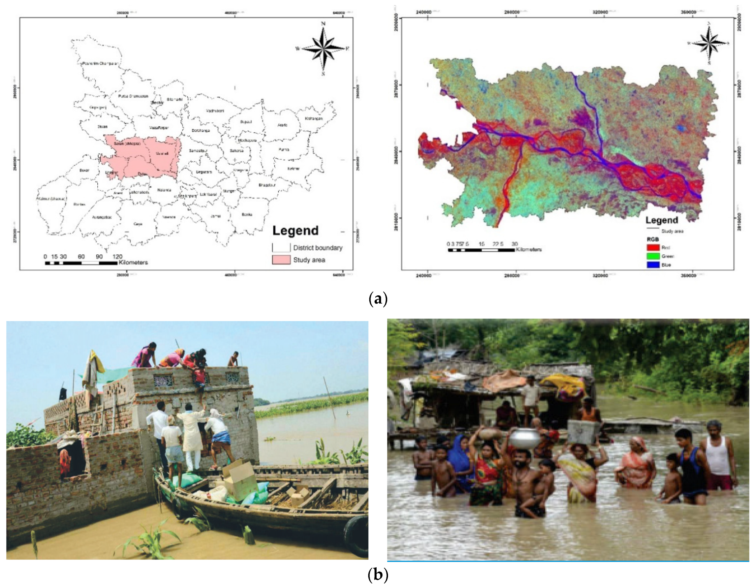
2.1. Study Area
2.2. Source of Data
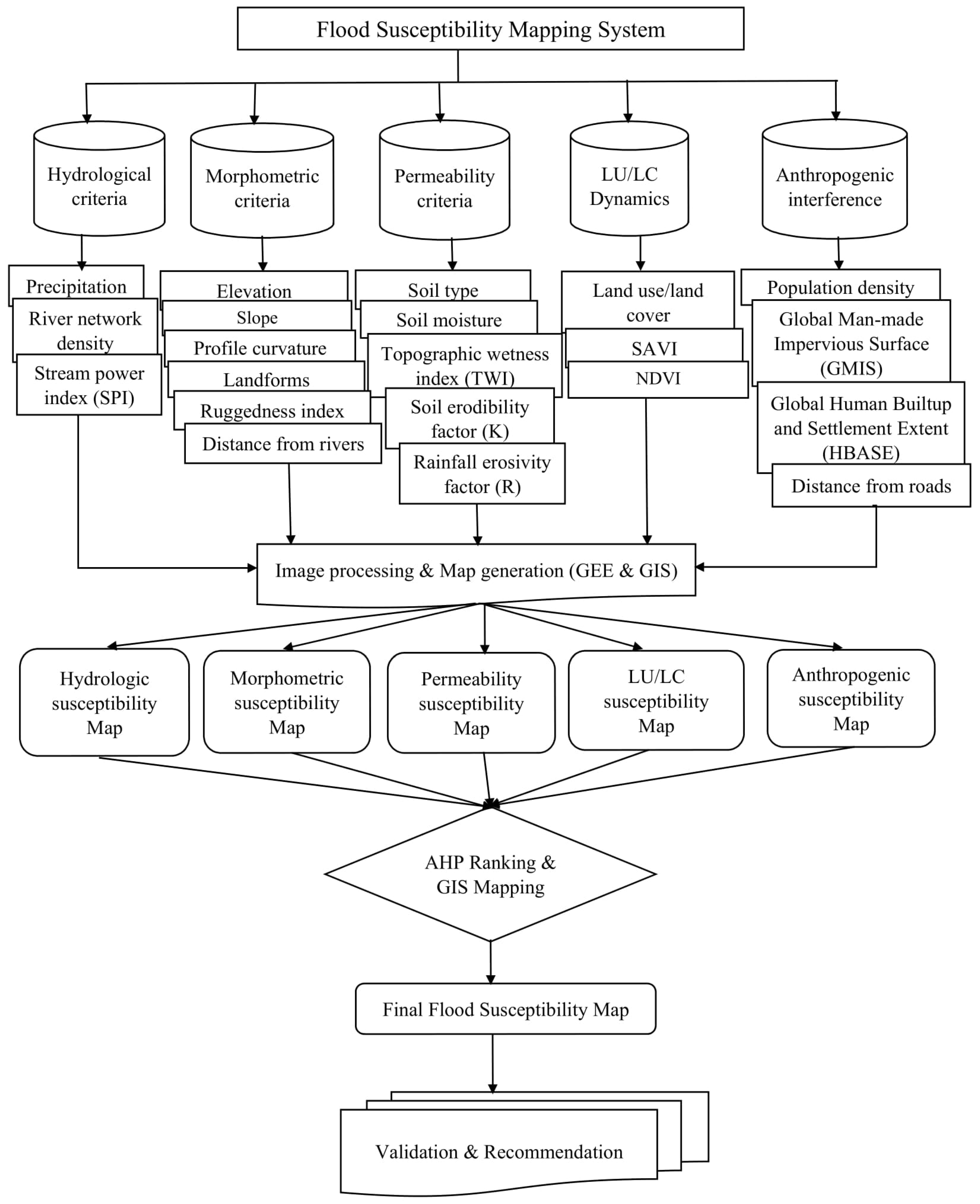
2.3. Flood Susceptibility Evaluation
2.3.1. Hydrological Criterion
2.3.2. Morphometric Criterion
2.3.3. Permeability
2.3.4. LU/LC Dynamics
2.3.5. Anthropogenic Interference
2.4. AHP Modeling Approaches
2.5. Validation of the Susceptibility Map
3. Results and Discussion
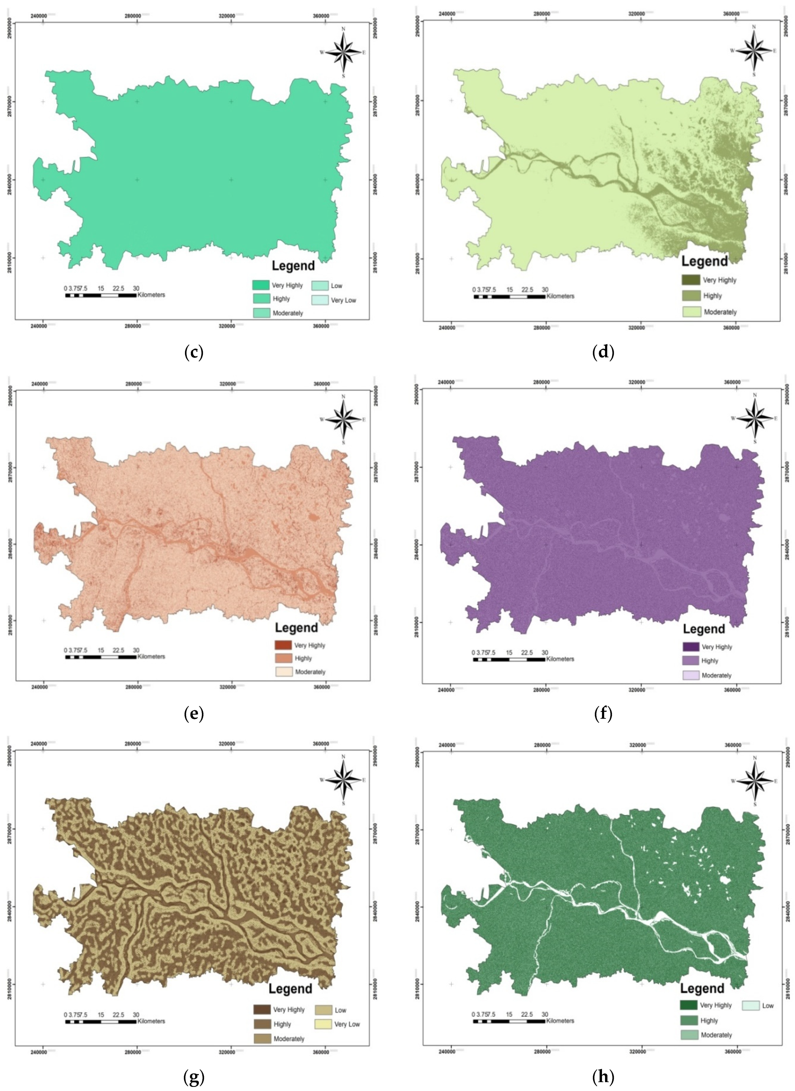
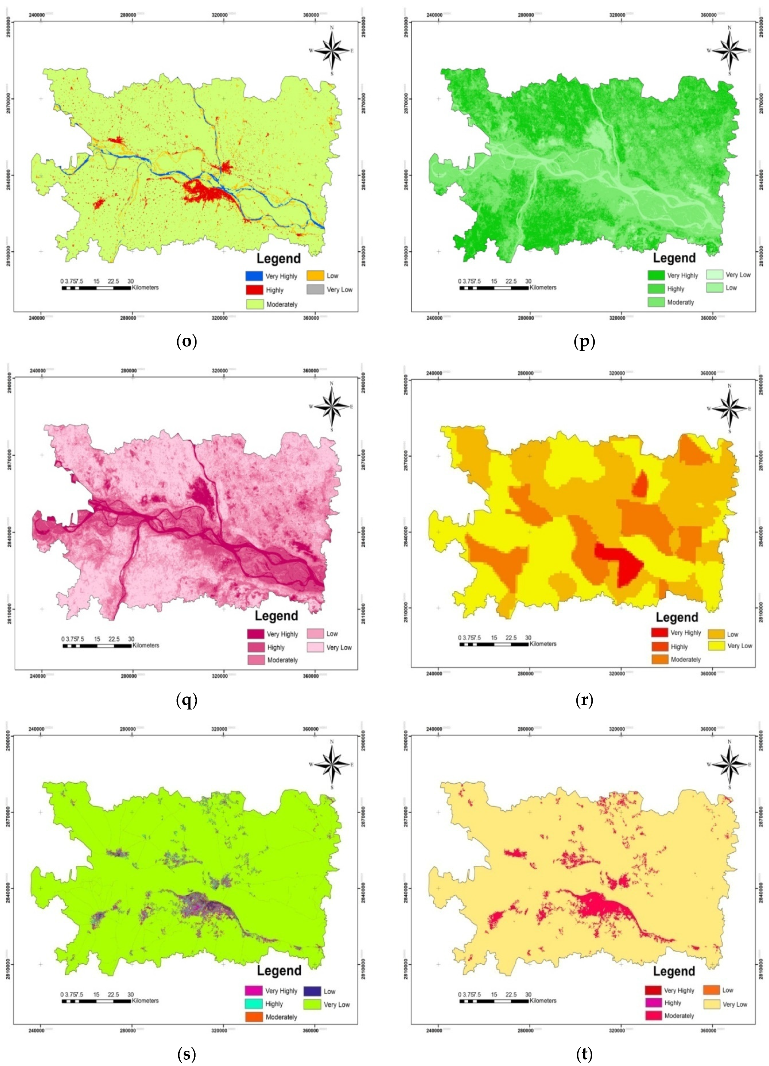
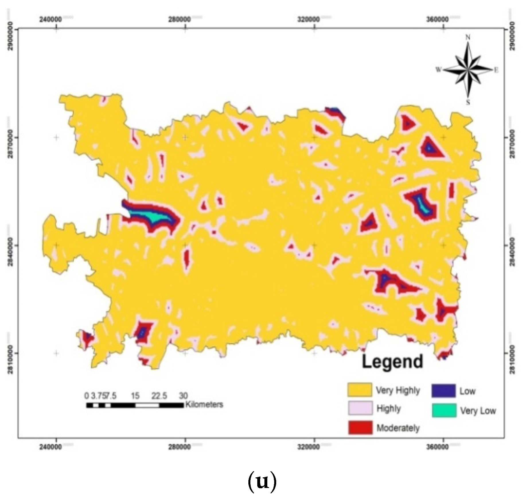
3.1. Flood Susceptibility Mapping
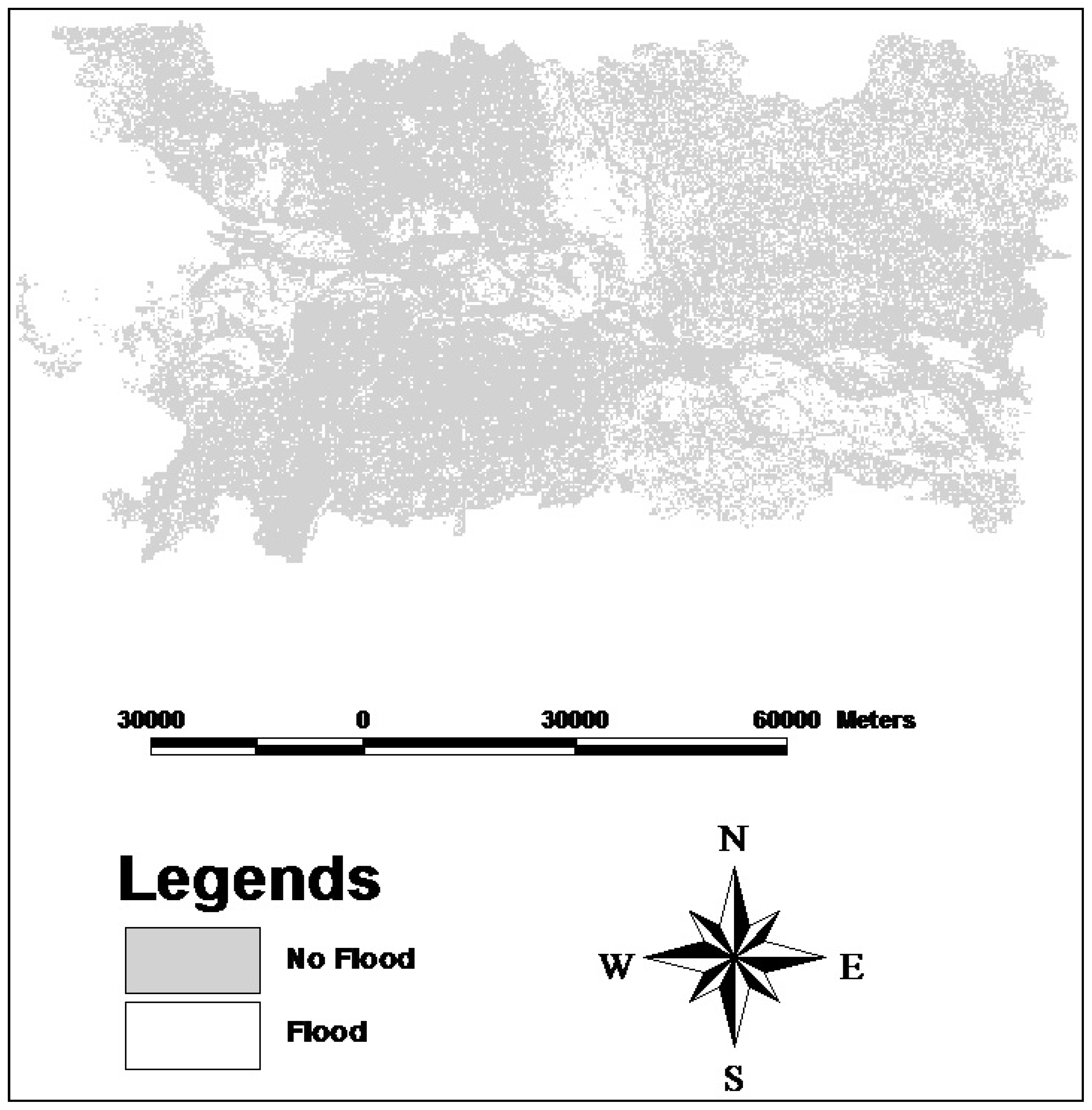
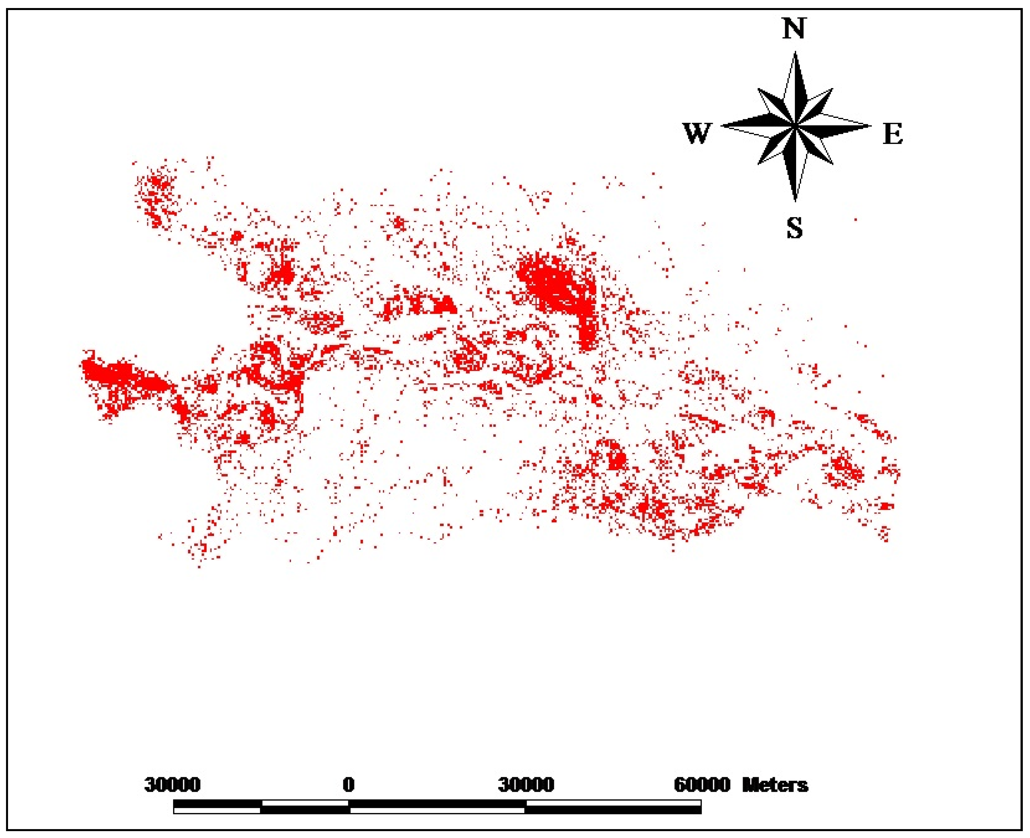
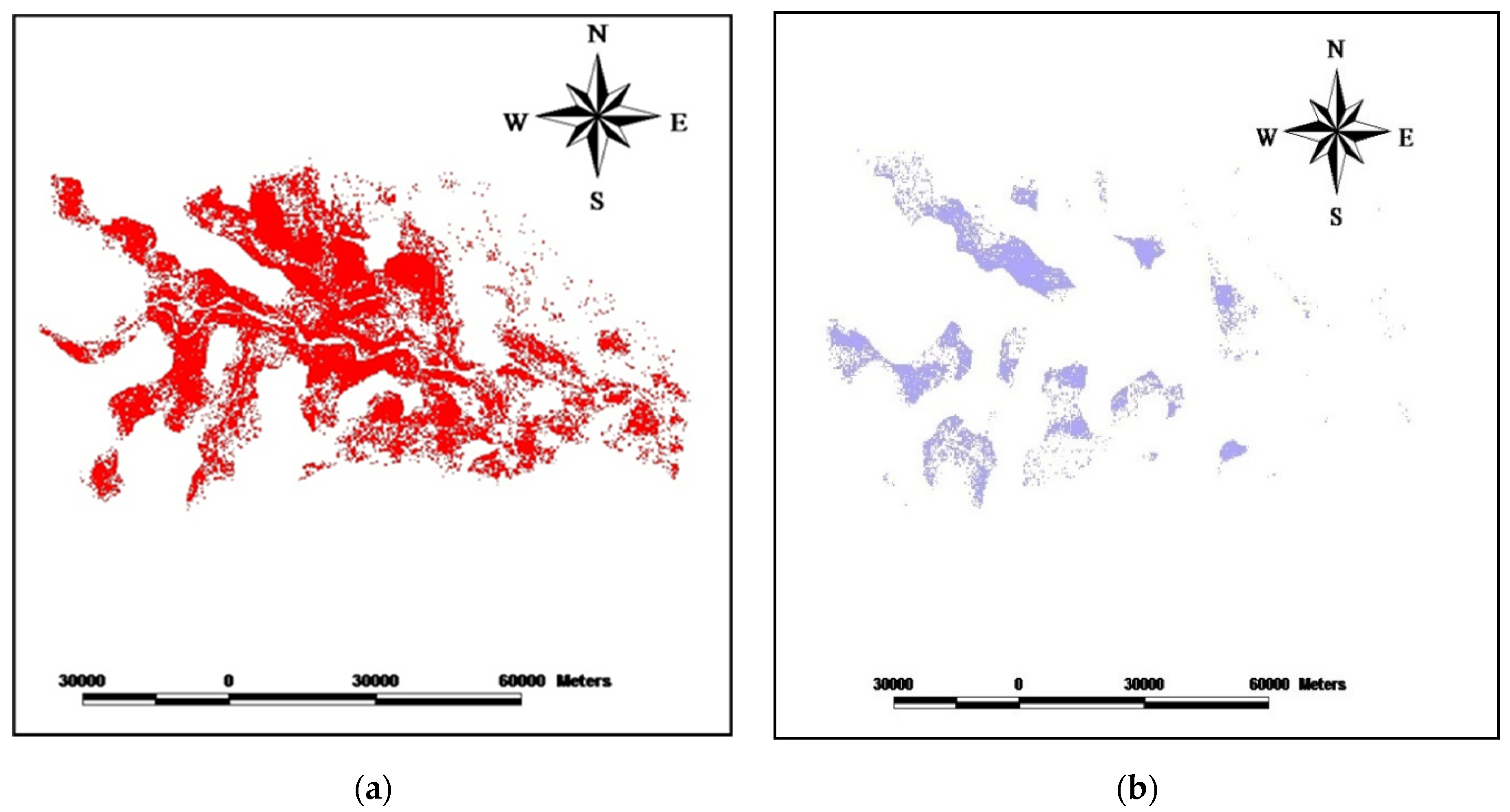
3.2. Validation with Sentinel 1 C Images
3.3. Flood Susceptible Zone near the River
3.4. Discussion
4. Conclusions
Author Contributions
Funding
Acknowledgments
Conflicts of Interest
References
- Giordan, D.; Notti, D.; Villa, A.; Zucca, F.; Calo, F.; Pepe, A. Low cost, multiscale and multi-sensor application for flooded area mapping. Nat. Hazards Earth Syst. Sci. 2018, 18, 1493–1516. [Google Scholar] [CrossRef]
- Sofia, G.; Roder, G.; Dalla Fontana, G.; Tarolli, P. Flood dynamics in urbanised landscapes: 100 years of climate and humans’ interaction. Sci. Rep. 2017, 7, 40527. [Google Scholar] [CrossRef] [PubMed]
- Smith, A.; Bates, P.D.; Wing, O.; Sampson, C.; Quinn, N.; Neal, J. New estimates of flood exposure in developing countries using high-resolution population data. Nat. Commun. 2019, 10, 1814. [Google Scholar] [CrossRef] [PubMed]
- Souissi, D.; Zouhri, L.; Hammami, S.; Msaddek, M.H.; Zghibi, A.; Dlala, M. GIS-based MCDM-AHP modeling for flood susceptibility mapping of arid areas, southeastern Tunisia. Geocarto Int. 2019, 35, 991–1017. [Google Scholar] [CrossRef]
- Pradhan, B. Flood susceptible mapping and risk area delineation using logistic regression, GIS and Remote sensing. J. Spat. Hydrol. 2009, 9, 1–18. [Google Scholar]
- Siahkamari, S.; Haghizadeh, A.; Zeinivand, H.; Tahmasebipour, N.; Rahmati, O. Spatial prediction of flood-susceptible areas using frequency ratio and maximum entropy models. Geocarto Int. 2018, 33, 927–941. [Google Scholar] [CrossRef]
- Shafapour-Tehrany, M.; Shabani, F.; NeamahJebur, M.; Hong, H.; Pourghasemi, H.R.; Xie, X. GIS-based spatial prediction of flood prone areas using standalone frequency ratio, logistic regression, weight of evidence and their ensemble techniques. Geomat. Nat. Hazards Risk 2017, 8, 1538–1561. [Google Scholar] [CrossRef]
- Liu, K.; Li, Z.; Yao, C.; Chen, J.; Zhang, K.; Saifullah, M. Coupling the k-nearest neighbor procedure with the Kalman filter for real-time updating of the hydraulic model in flood forecasting. Int. J. Sediment Res. 2016, 31, 149–158. [Google Scholar] [CrossRef]
- Dano, U.; Balogun, A.L.; Matori, A.N.; Wan Yusouf, K.; Rimi Abubakar, I.; Said Mohamed, M.; Pradhan, B. Flood Susceptibility Mapping Using GIS-Based Analytic Network Process: A Case Study of Perlis, Malaysia. Water 2019, 11, 615. [Google Scholar] [CrossRef]
- Li, Y.; Martinis, S.; Wieland, M.; Schlaffer, S.; Natsuaki, R. Urban Flood Mapping Using SAR Intensity and Interferometric Coherence via Bayesian Network Fusion. Remote Sens. 2019, 11, 2231. [Google Scholar] [CrossRef]
- Darabi, H.; Choubin, B.; Rahmati, O.; Haghighi, A.T.; Pradhan, B.; Kløve, B. Urban flood risk mapping using the GARP and QUEST models: A comparative study of machine learning techniques. J. Hydrol. 2019, 569, 142–154. [Google Scholar] [CrossRef]
- Termeh, S.V.R.; Kornejady, A.; Pourghasemi, H.R.; Keesstra, S. Flood susceptibility mapping using novelensembles of adaptive neuro fuzzy inference system and metaheuristic algorithms. Sci. Total Environ. 2018, 615, 438–451. [Google Scholar] [CrossRef] [PubMed]
- Rahmati, O.; Zeinivand, H.; Besharat, M. Flood hazard zoning in Yasooj region, Iran, using GIS and multi-criteria decision analysis. Geomat. Nat. Hazards Risk 2016, 7, 1000–1017. [Google Scholar] [CrossRef]
- Oeurng, C.; Sauvage, S.; Sánchez-Pérez, J.M. Assessment of hydrology, sediment and particulate organic carbon yield in a large agricultural catchment using the SWAT model. J. Hydrol. 2011, 401, 145–153. [Google Scholar] [CrossRef]
- Choubin, B.; Moradi, E.; Golshan, M.; Adamowski, J.; Sajedi-Hosseini, F.; Mosavi, A. An ensemble prediction of flood susceptibility using multivariate discriminant analysis, classification and regression trees, and support vector machines. Sci. Total Environ. 2019, 651, 2087–2096. [Google Scholar] [CrossRef]
- Hong, H.; Tsangaratos, P.; Ilia, I.; Liu, J.; Zhu, A.X.; Chen, W. Application of fuzzy weight of evidence and data mining techniques in construction of flood susceptibility map of Poyang County, China. Sci. Total Environ. 2018, 625, 575–588. [Google Scholar] [CrossRef]
- Khosravi, K.; Pham, B.T.; Chapi, K.; Shirzadi, A.; Shahabi, H.; Revhaug, I.; Prakash, I.; Bui, D.T. A comparative assessment of decision trees algorithms for flash flood susceptibility modeling at Haraz watershed, Northern Iran. Sci. Total Environ. 2018, 627, 744–755. [Google Scholar] [CrossRef]
- Wang, Y.; Fang, Z.; Hong, H.; Peng, L. Flood susceptibility mapping using convolutional neural network frameworks. J. Hydrol. 2020, 582, 124482. [Google Scholar] [CrossRef]
- Jahangir, M.H.; Reineh, S.M.M.; Abolghasemi, M. Spatial predication of flood zonation mapping in Kan River Basin, Iran, using artificial neural network algorithm. Weather Clim. Extrem. 2019, 25, 100215. [Google Scholar] [CrossRef]
- Duan, Q.; Sorooshian, S.; Gupta, V. Effective and efficient global optimization for conceptual rainfall-runoff models. Water Resour. Res. 1992, 28, 1015–1031. [Google Scholar] [CrossRef]
- Bahrami, S. Global Ensemble Stream Flow and Flood Modeling with Application of Large Data Analytics, Deep Learning and GIS. Unpublished Master’s Thesis, University of Naved, Reno, NV, USA, 2019; p. 210. [Google Scholar]
- Tellman, B.; Kuhn, C.; Max, S.A.; Sullivan, J. Dynamic Flood Vulnerability Mapping with Google Earth Engine. In Proceedings of the American Geophysical Union Fall Meeting, San Francisco, CA, USA, 14–18 December 2015; pp. 5523–5527. [Google Scholar]
- Liu, C.C.; Shieh, M.C.; Ke, M.S.; Wang, K.H. Flood Prevention and Emergency Response System Powered by Google Earth Engine. Remote Sens. 2018, 10, 1283. [Google Scholar] [CrossRef]
- Vojtek, M.; Vojteková, J. Flood Susceptibility Mapping on a National Scale in Slovakia Using the Analytical Hierarchy Process. Water 2019, 11, 364. [Google Scholar] [CrossRef]
- Yahaya, S.; Ahmad, N.; Abdalla, R.F. Multicriteria analysis for flood vulnerable areas in Hadejia-Jama’are River basin, Nigeria. Eur. J. Sci. Res. 2010, 42, 71–83. [Google Scholar]
- India Water Portal. Bihar Floods 2008 Archived 1 February 2009 at the Wayback Machine. 2009. Available online: https://www.indiawaterportal.org/ (accessed on 2 February 2020).
- GhorbaniNejad, S.; Falah, F.; Daneshfar, M.; Haghizadeh, A.; Rahmati, O. Delineation of groundwater potential zones using remote sensing and GIS-based data-driven models. Geocarto Int. 2017, 32, 167–187. [Google Scholar]
- Shahabi, H.; Shirzadi, A.; Ghaderi, K.; Omidvar, E.; Al-Ansari, N.; Clague, J.J.; Geertsema, M.; Khosravi, K.; Amini, A.; Bahrami, S.; et al. Flood Detection and Susceptibility Mapping Using Sentinel-1 Remote Sensing Data and a Machine Learning Approach: Hybrid Intelligence of Bagging Ensemble Based on K-Nearest Neighbor Classifier. Remote Sens. 2020, 12, 266. [Google Scholar] [CrossRef]
- Fernández, D.S.; Lutz, M.A. Urban flood hazard zoning in Tucumán Province, Argentina, using GIS and multicriteria decision analysis. Eng. Geol. 2010, 111, 90–98. [Google Scholar] [CrossRef]
- Beven, K.J.; Kirkby, M.J.A. Physically based, variable contributing area model of basin hydrology/Un modèle à base physique de zone d’appel variable de l’hydrologie du basin versant. Hydrol. Sci. J. 1979, 24, 43–69. [Google Scholar] [CrossRef]
- Bilskie, M.V.; Hagen, S.C.; Medeiros, S.C.; Passeri, D.L. Dynamics of sea level rise and coastal flooding on a changing landscape. Geophy. Res. Lett. 2014, 41, 927–934. [Google Scholar] [CrossRef]
- Kourgialas, N.N.; Karatzas, G.P. Flood management and a GIS modelling method to assess flood-hazard areas—A case study. Hydrol Sci. J. 2011, 56, 212–225. [Google Scholar] [CrossRef]
- Tehrany, M.S.; Pradhan, B.; Jebur, M.N. Flood susceptibility mapping using a novel ensemble weights-of-evidence and support vector machine models in GIS. J. Hydrol. 2014, 512, 332–343. [Google Scholar] [CrossRef]
- Malinowski, R.; Groom, G.; Schwanghart, W.; Heckrath, G. Detection and Delineation of Localized Flooding from WorldView-2 Multispectral Data. Remote Sens. 2015, 7, 14853–14875. [Google Scholar] [CrossRef]
- CIESIN. Center for International Earth Science Information Network, Gridded Population of the World (GPWv3); CIESIN, Columbia University, and Centro Internacional de Agricultura Tropical: Palisades, NY, USA, 2005. [Google Scholar]
- Jebur, M.N.; Pradhan, B.; Tehrany, M.S. Optimization of landslide conditioning factors using very high-resolution airborne laser scanning (LiDAR) data at catchment scale. Remote Sens. Environ. 2014, 152, 150–165. [Google Scholar] [CrossRef]
- Diwakar, S.K.; Nagarkoti, J. Performance of WRF (ARW) over River Basins under Flood Met Office, Patna during Flood Season-2014; Indian Meteorological Department: New Delhi, India, 2016; p. 30. [CrossRef]
- FMIS. Flood Management Information System (FMIS), Water Resource Department, Bihar. 2019. Available online: http://fmis.bih.nic.in/mapWRD_INUN.html (accessed on 8 May 2019).
- Dube, M. Bihar Floods: A Report on Bihar Floods 2016; Bihar Disaster Management Authority, Government of Bihar: Patna, India, 2018; p. 36.
- Drobot, R. Methodology for Determining Torrential Catchments in Which Human Settlements Are Exposed to Flash Floods; Technical University of Civil Engineering: Bucharest, Romania, 2007. (In Romanian) [Google Scholar]
- Amin, K. Application of Remote Sensing and GIS in Flash Flood Hazard Mapping and Hydraulic Design (Case Study of Wadi Dahdah, Saudi Arabia). 2019. Available online: https://www.academia.edu/20126182/Application_of_Remote_Sensing_and_GIS_for_Floodplain_mapping_and_Hydraulic_design (accessed on 1 January 2020).
- Al-Saady, Y.I.; Al-Suhail, Q.A.; Al-Tawash, B.S.; Othman, A.A. Drainage network extraction and morphometric analysis using remote sensing and GIS mapping techniques (Lesser Zab River Basin, Iraq and Iran). Environ. Earth Sci. 2016, 75, 1243. [Google Scholar] [CrossRef]
- Musy, A.; Higy, C. Hydrology. A Science of Nature; CRC Press, Taylor & Francis Group, Science Publishers: Enfield, NH, USA, 2011. [Google Scholar]
- Ochoa, P.; Fries, A.; Mejía, D.; Burneo, J.; Ruíz-Sinoga, J.; Cerdà, A. Effects of climate, land cover and topography on soil erosion risk in a semiarid basin of the Andes. Catena 2016, 140, 31–42. [Google Scholar] [CrossRef]
- Renard, K.G.; Foster, G.R.; Weesies, G.A. Predicting soil erosion by water: A guide to conservation planning with the revised universal soil loss equation (RUSLE). In Agriculture Handbook Number 703; USDA-ARS: Washington, DC, USA, 1997; p. 404. [Google Scholar]
- Goffi, A.; Stroppiana, D.; Brivio, P.A.; Bordogna, G.; Boschetti, M. Towards an automated approach to map flooded areas from Sentinel-2 MSI data and soft integration of water spectral features. Int. J. Appl. Earth Obs. Geoinf. 2020, 84, 101951. [Google Scholar] [CrossRef]
- Tucker, C.J. Red and photographic infrared linear combinations for monitoring vegetation. Remote Sens. Environ. 1979, 8, 127–150. [Google Scholar] [CrossRef]
- Huete, A.R. A soil-adjusted vegetation index (SAVI). Remote Sens. Environ. 1988, 25, 295–309. [Google Scholar] [CrossRef]
- Center for International Earth Science Information Network—CIESIN—Columbia University (CIESIN). Gridded Population of the World, Version 4 (GPWv4): Basic Demographic Characteristics, Revision 11; NASA Socioeconomic Data and Applications Center (SEDAC): Palisades, NY, USA, 2018; Available online: https://sedac.ciesin.columbia.edu/data/collection/gpw-v4 (accessed on 10 May 2019). [CrossRef]
- Pesaresi, M.; Ehrilch, D.; Florczyk, A.J.; Freire, S.; Julea, A. GHS Built-Upgrid, Derived from Landsat, Multitemporal (1975, 1990, 2000, 2014) (versionR2015); European Commission, Joint Research Centre (JRC): Ispra, Italy, 2019; Available online: http://data.europa.eu/89h/jrc-ghsl-hs_built_ldsmt_globe_r2015b (accessed on 21 April 2019).
- Ayalew, L.; Yamagishi, H. The application of GIS-based logistic regression for landslide susceptibility mapping in the Kakuda–Yahiko Mountains, Central Japan. Geomorpho 2005, 65, 15–31. [Google Scholar] [CrossRef]
- Singha, C.; Swain, K.C. Land Suitability Evaluation Criteria for Agricultural crop selection: A Review. Agric. Rev. 2016, 37, 125–132. [Google Scholar] [CrossRef]
- Saaty, T.L. The Analytical Hierarchy Process; McGraw Hill: New York, NY, USA, 1980. [Google Scholar]
- Luu, C.; Von Meding, J.; Kanjanabootra, S. Assessing flood hazard using flood marks and analytic hierarchy process approach: A case study for the 2013 flood event in Quang Nam, Vietnam. Nat. Hazards 2018, 90, 1031–1050. [Google Scholar] [CrossRef]
- Saaty, T.L.; Vargas, G.L. Models, Methods, Concepts, and Applications of the Analytic Hierarchy Process. Int. Ser. Oper. Res. Manag. Sci. 2001, 32, 93. [Google Scholar] [CrossRef]
- Drobne, S.; Lisec, A. Multi-attribute decision analysis in GIS: Weighted linear combination and ordered weighted averaging. Informatica 2009, 33, 459–474. [Google Scholar]
- Singha, C.; Swain, K.C.; Saren, B.K. Land Suitability Assessment for Potato Crop using Analytic Hierarchy Process Technique and Geographic Information System. J. Agric. Eng. 2019, 56, 78–87. Available online: http://www.isae.in/journal_jae.aspx (accessed on 10 August 2020).
- Al-Abadi, A.M.; Shahid, S.; Al-Ali, A.K.A. GIS-based integration of catastrophe theory and analytical hierarchy process for mapping flood susceptibility: A case study of Teeb area, Southern Iraq. Environ. Earth Sci. 2016, 75, 687. [Google Scholar] [CrossRef]
- Santangelo, N.; Santo, A.; Di Crescenzo, G.; Foscari, G.; Liuzza, V.; Sciarrotta, S.; Scorpio, V. Flood susceptibility assessment in a highly urbanized alluvial fan: The case study of Sala Consilina (southern Italy). Nat. Hazards Earth Syst. Sci. 2011, 11, 2765–2780. [Google Scholar] [CrossRef]
- Seejata, K.; Yodying, A.; Wongthadam, T.; Mahavik, N.; Tantanee, S. Assessment of flood hazard areas using Analytical Hierarchy Process over the Lower Yom Basin, Sukhothai Province. Procedia Eng. 2018, 212, 340–347. [Google Scholar] [CrossRef]
- Tanga, X.; Lib, J.; Liuc, M.; Liud, W.; Hong, H. Flood susceptibility assessment based on a novel random Naïve Bayes method: A comparison between different factor discretization. Catena 2019, 189, 104536. [Google Scholar] [CrossRef]
- Chen, W.; Li, Y.; Xue, W.; Shahabi, H.; Li, S.; Hong, H.; Bin Ahmad, B. Modeling flood susceptibility using data-driven approaches of naïve Bayes tree, alternating decision tree, and random forest methods. Sci. Total Environ. 2019, 701, 134979. [Google Scholar] [CrossRef]
- Sahana, M.; Rehman, S.; Sajjad, H.; Hong, H. Exploring effectiveness of frequency ratio and support vector machine models in storm surge flood susceptibility assessment: A study of Sundarban Biosphere Reserve, India. Catena 2020, 189, 104450. [Google Scholar] [CrossRef]


| Year | Human | Animals | Year | Human | Animals |
|---|---|---|---|---|---|
| 2019 | 1885 | 755 | 2005 | 58 | 4 |
| 2018 | 1476 | 643 | 2004 | 885 | 3272 |
| 2017 | 1521 | 792 | 2003 | 251 | 108 |
| 2016 | 1254 | 5383 | 2002 | 489 | 1450 |
| 2013 | 1201 | 140 | 2001 | 231 | 565 |
| 2008 | 2534 | 845 | 2000 | 336 | 2568 |
| 2007 | 1287 | 126 | 1999 | 243 | 136 |
| 2006 | 36 | 31 |
| SL No. | Data Type | Description | Source |
|---|---|---|---|
| 1 | DEM | ASTER DEM (30 m) | usgs.gov.in |
| 2 | Landforms | Global ALOS Landforms (30 m) | USGS/Google Earth Engine |
| 3 | Precipitation (mm/day) | TRMM (0.25°) | https://giovanni.gsfc.nasa.gov/giovanni/ |
| 4 | Soil data | Soil Region and sub order associations of India; RF 1:7,000,000 | NBSS and LUP, Nagpur |
| 5 | Soil moisture | SMAP L-band radiometer data, version 1.0 beta (40 km) | https://www.mosdac.gov.in/ |
| Soil erodibility (K) and rainfall erosivity (R)factor | RUSLE-based Global Soil Erosion Modelling platform (GloSEM; version 1.1), 25 km | https://esdac.jrc.ec.europa.eu/content/globalsoilerosion | |
| 6 | Landsat 8 Images | LANDSAT/LC08/C01/T1_TOA (30 m) | USGS/Google Earth Engine |
| 7 | Land cover | COPERNICUS/Landcover/100 m/Proba-V/Global | https://developers.google.com/earth-engine/datasets |
| 8 | Population Density | The Gridded Population of the World, Version 4 (GPWv4) (30 arc s) | https://sedac.ciesin.columbia.edu/data/collection/gpw-v4 |
| 9 | GMIS | Global Man-made Impervious Surface (Landsat, v1) | https://sedac.ciesin.columbia.edu/data/set/ulandsat-gmis-v1 |
| 10 | HBASE | Global Human Built-up and Settlement Extent (Landsat, v1) | https://sedac.ciesin.columbia.edu/data/set/ulandsat-hbase-v1 |
| 11 | Road network | Road network in Bihar | https://www.openstreetmap.org/export#map=9/25.4172/85.1660 |
| Flood Causative Criterion | Susceptibility Class Ranges and Ratings | |||||
|---|---|---|---|---|---|---|
| Unit | Very High (5) | High (4) | Moderate (3) | Low (2) | Very Low (1) | |
| (A) Hydrologic criterion | ||||||
| Precipitation | mm | >7.50 | 7.0–7.50 | 6.50–7.0 | 6.0–6.50 | <6.0 |
| River network density | km/km2 | >1.53 | 1.26–1.52 | 1.00–1.25 | 0.70–0.99 | 0–0.69 |
| Stream power index (SPI) | level | 0–0.005 | 0.006–0.642 | 0.643–0.990 | 0.990–1.500 | >1.500 |
| (B) Morphometric criterion | ||||||
| Elevation | m | 0–20 | 20–50 | 50–100 | 100–150 | >150 |
| Slope | (°) | 0.0–2 | 2.1–5.0 | 5.1–15.0 | 15.1–35.0 | >35 |
| Profile curvature | radians/m | 0–0.25 | 0.26–0.90 | 0.91–2.5 | 2.56–3.00 | 3.00–3.50 |
| Landforms | level | Valley, Valley (narrow) | Lower slope (flat) | Upper slope (warm) | Upper slope, Upper slope (flat) | Peak/ridge (warm) |
| Ruggedness index | level | 0.11–0.32 | 0.33–0.42 | 0.43–0.51 | 0.52–0.60 | 0.60–0.88 |
| Distance from rivers | m | <200 | 200–500 | 501–1000 | 1001–1500 | >2000 |
| (C) Permeability | ||||||
| Soil type | level | Silty clay | Limestone and Marly, Limestone and Dlomies, Limestone Marly, and Gypsum | Alluvium, Silty sediments and Quaternary sediments | Sandy clay sand and conglomerate | Coarse sand |
| Soil Moisture | Average % | 30.01–35.0 | 25.01–30.00 | 20.01–25.00 | 15.01–20.00 | 0–15.00 |
| Topographic wetness index (TWI) | level | >20.01 | 15.01–20.00 | 10.01–15.00 | 0.001–10.00 | <0.001 |
| Soil erodibility factor (K) | level | >0.175 | 0.170–0.175 | 0.133–0.169 | 0.107–0.132 | <0.106 |
| Rainfall erosivity factor (R) | level | >5000 | 4500–5000 | 4200–4500 | 4000–4200 | <4000 |
| (D) Landcover Dynamics | ||||||
| Landuse and landcover (LU/LC) | level | River, urban | Agriculture land | Wet land, shrubs, bare land | Low vegetation | Mixed forest |
| SAVI | level | −0.50 to −0.30 | −0.29 to −0.22 | −0.22 to −0.13 | −0.12 to −0.02 | −0.02 to 0.14 |
| NDVI | level | >−0.02 | −0.02 to 0.30 | 0.31–0.40 | 0.41–0.50 | 0.51–0.65 |
| (E) Anthropogenic interference | ||||||
| Population density | Person/km2 | >8000 | 6001–8000 | 4001–6000 | 2001–4000 | 2000 |
| Human built-up extent | level | >200 | 151–200 | 101–150 | 51–100 | 0–50 |
| Impervious area | % | >150 | 101–150 | 51–100 | 21–50 | 0–20 |
| Distance to road network | m | 0–25 | 26–50 | 51–100 | 101–150 | >150 |
| Hydrological Criterion | Morphometric Criterion | Land Cover Dynamics | Permeability | Anthropogenic Interference | Weightage | |
|---|---|---|---|---|---|---|
| Hydrological criterion | 1 | 3 | 5 | 6 | 8 | 0.497 |
| Morphometric criterion | 0.33 | 1 | 3 | 4 | 7 | 0.259 |
| Land cover dynamics | 0.2 | 0.33 | 1 | 2 | 5 | 0.128 |
| Permeability | 0.167 | 0.25 | 0.5 | 1 | 3 | 0.079 |
| Anthropogenic interference | 0.125 | 0.143 | 0.2 | 0.333 | 1 | 0.037 |
| Criteria | Very High, sq km | % | High, sq km | % | Moderate, sq km | % | Low, sq km | % | Very Low, sq km | % |
|---|---|---|---|---|---|---|---|---|---|---|
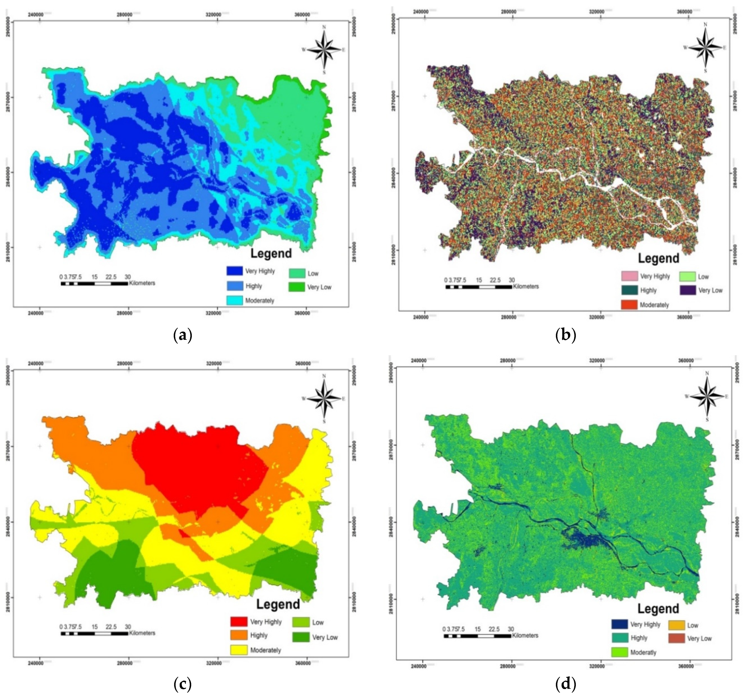
| Hydrologic | 2057.73 | 27.8 | 2531.3 | 34.3 | 1324.36 | 17.9 | 1355.2 | 18.3 | 119.44 | 1.62 |
| Morphometric | 405.83 | 5.49 | 1389.1 | 18.8 | 1965.14 | 26.6 | 2118.7 | 28.7 | 1509.28 | 20.4 |
| Permeability | 1513.60 | 20.5 | 1773.4 | 24.0 | 2084.08 | 28.2 | 1104.0 | 14.9 | 912.94 | 12.4 |
| Land cover dynamics | 314.20 | 4.3 | 5117.9 | 69.2 | 1897.84 | 25.6 | 57.42 | 0.78 | 0.55 | 0.01 |
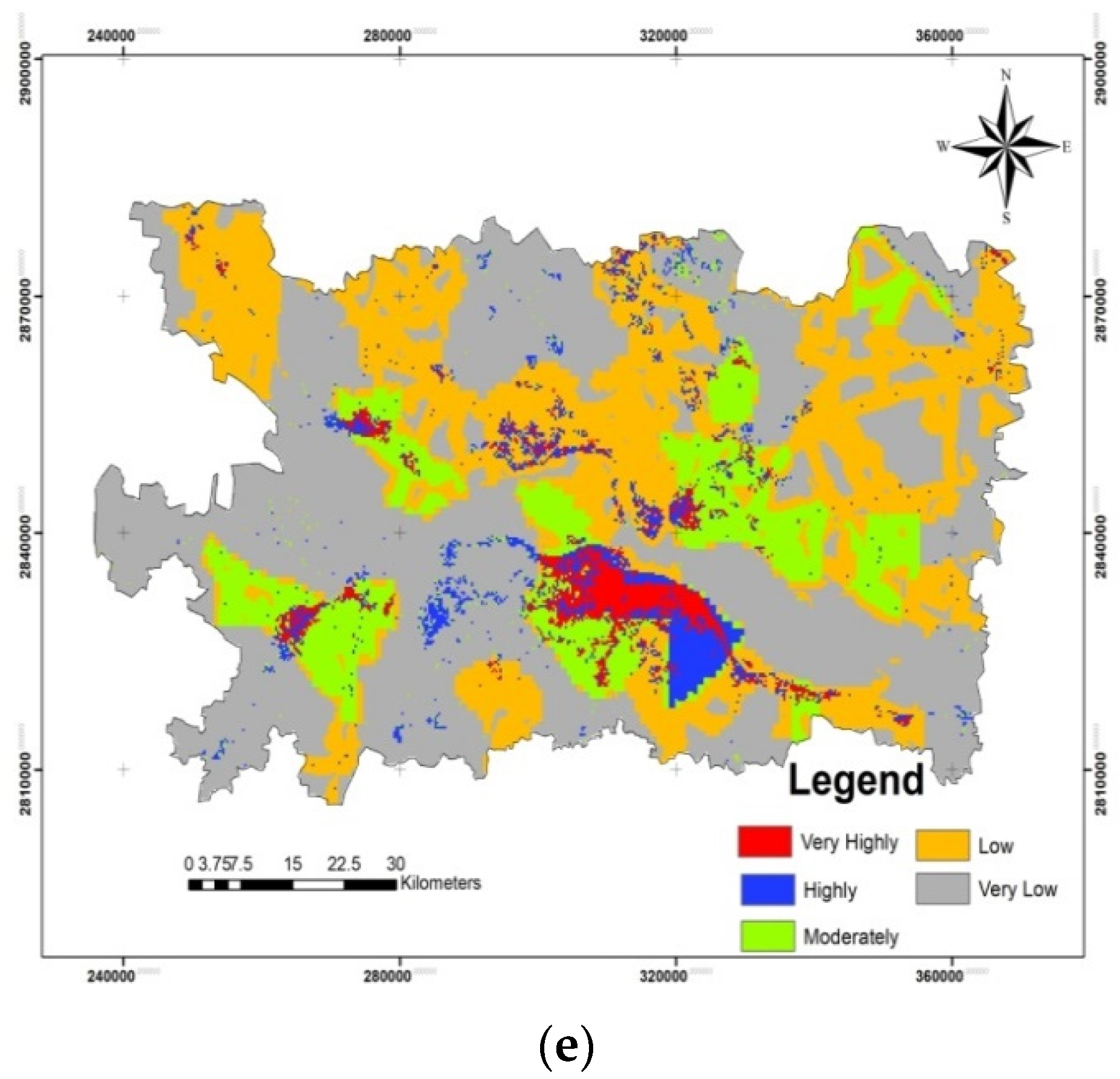
| Anthropogenic | 159.290 | 2.2 | 294.22 | 3.98 | 906.82 | 12.2 | 2346.3 | 31.7 | 3681.27 | 49.8 |
| Final flood susceptibility | 1002.710 | 13.6 | 1978.9 | 26.7 | 1956.17 | 26.5 | 1536.6 | 20.8 | 913.49 | 12.4 |
Publisher’s Note: MDPI stays neutral with regard to jurisdictional claims in published maps and institutional affiliations. |
© 2020 by the authors. Licensee MDPI, Basel, Switzerland. This article is an open access article distributed under the terms and conditions of the Creative Commons Attribution (CC BY) license (http://creativecommons.org/licenses/by/4.0/).
Share and Cite
Swain, K.C.; Singha, C.; Nayak, L. Flood Susceptibility Mapping through the GIS-AHP Technique Using the Cloud. ISPRS Int. J. Geo-Inf. 2020, 9, 720. https://doi.org/10.3390/ijgi9120720
Swain KC, Singha C, Nayak L. Flood Susceptibility Mapping through the GIS-AHP Technique Using the Cloud. ISPRS International Journal of Geo-Information. 2020; 9(12):720. https://doi.org/10.3390/ijgi9120720
Chicago/Turabian StyleSwain, Kishore Chandra, Chiranjit Singha, and Laxmikanta Nayak. 2020. "Flood Susceptibility Mapping through the GIS-AHP Technique Using the Cloud" ISPRS International Journal of Geo-Information 9, no. 12: 720. https://doi.org/10.3390/ijgi9120720
APA StyleSwain, K. C., Singha, C., & Nayak, L. (2020). Flood Susceptibility Mapping through the GIS-AHP Technique Using the Cloud. ISPRS International Journal of Geo-Information, 9(12), 720. https://doi.org/10.3390/ijgi9120720