Density-Based Spatial Clustering and Ordering Points Approach for Characterizations of Tourist Behaviour

 , , , , and
Abstract
1. Introduction
2. Materials and Methods
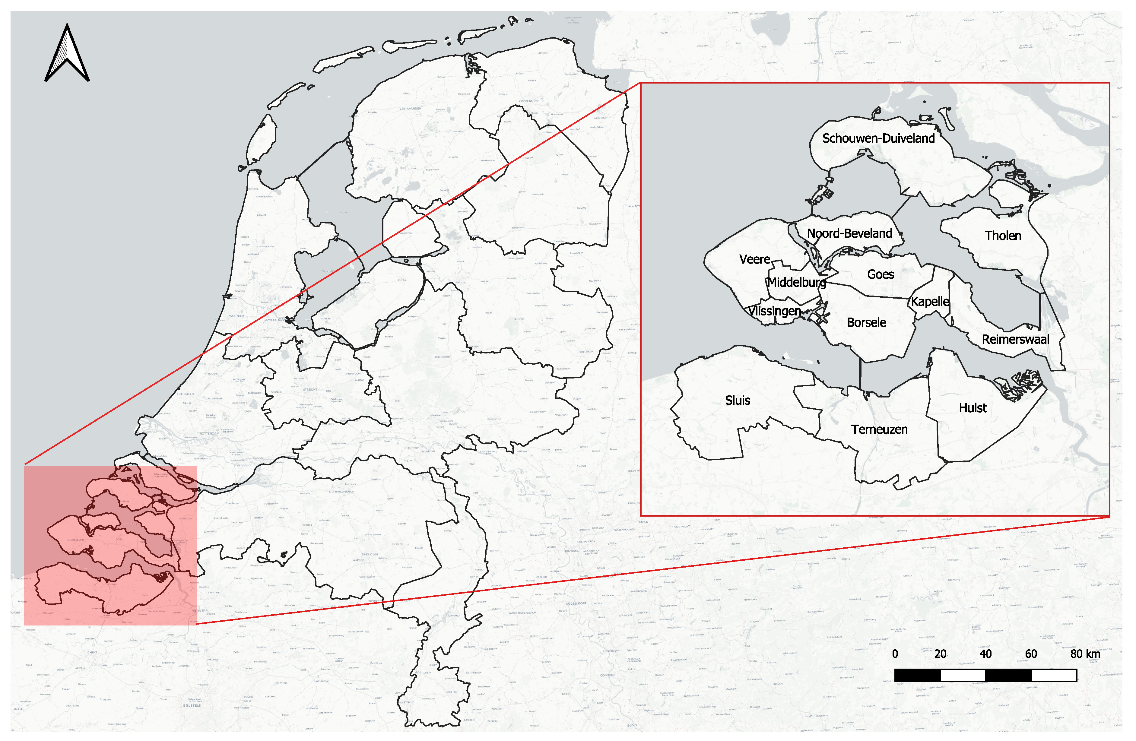
2.1. Geographical Study Area
2.2. Dataset
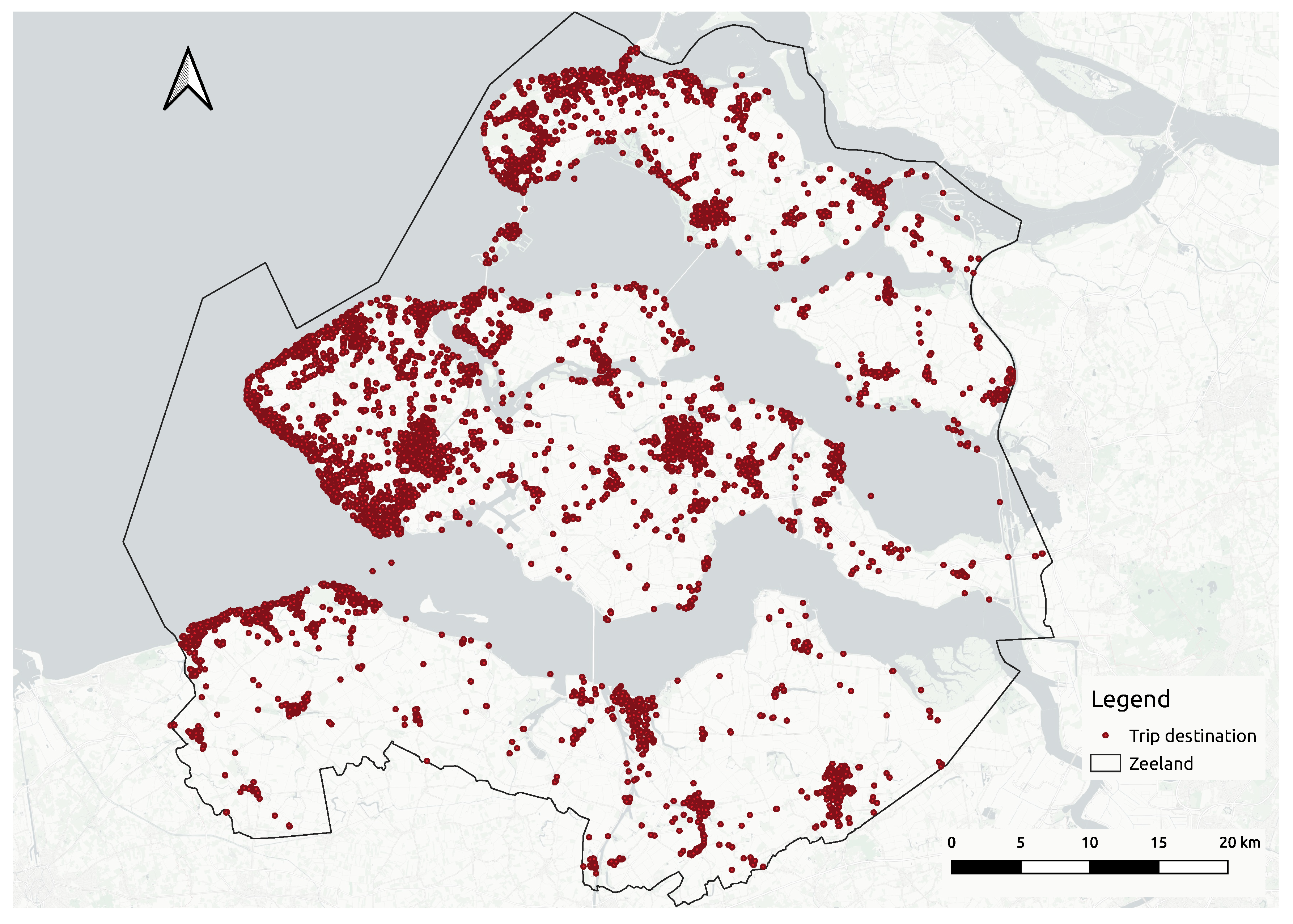
- Crowdsourced tourist dataset. The data were collected by the mobile crowdsourced application provided by the official regional tourist information agency VVV Zeeland (Province of Zeeland, The Netherlands). The target users were tourists visiting the province from May to September 2017. During this period, a total of 10,597 users downloaded the application, of which 1505 contributed their data. The active users contributed 124,725 trips (travelled path from the trip origin to the trip destination location), and 151,612 trip segments (parts of the trip made by single transport mode). In the dataset, each record represents a trip segment. A detailed description of attributes collected for each trip segment is given in Table 1.
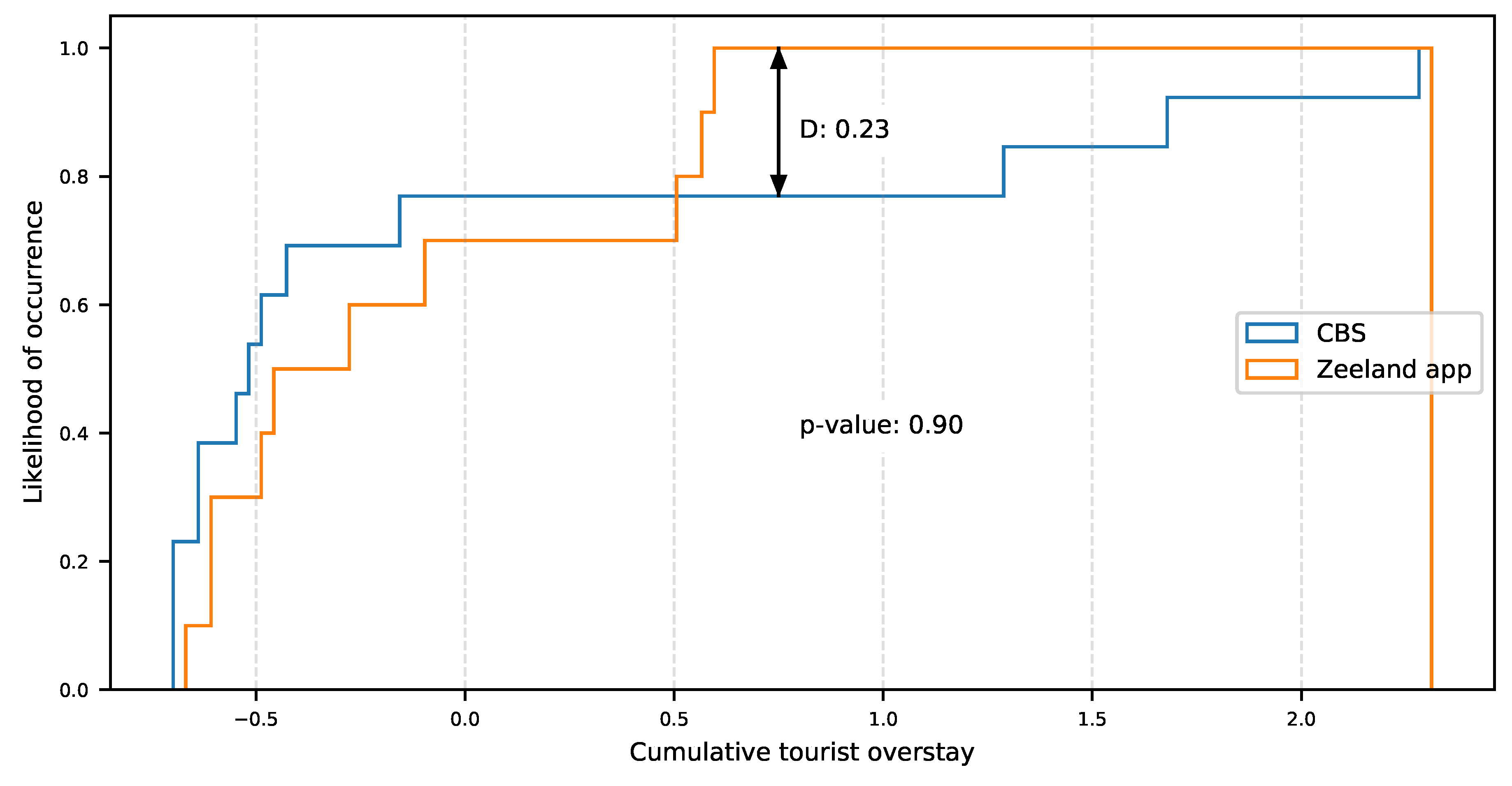
- CBS dataset. This dataset consists of the statistics published by CBS about the tourists in accommodations of the Province of Zeeland [24]. The time period considered in the comparison is from July to September 2017. This external data source is used to measure the representativeness of the crowdsourced data.
- Land-use of The Netherlands. This dataset consists of the land-use file from The Netherlands published by CBS [25]. It contains digital geometry of land use such as traffic areas, buildings, and recreation areas. This external data source is used to complement the dataset to be able to to give a data-driven interpretation to the results. Table 2 shows the dataset fields.
- Validation dataset. NBTC-NIPO Research is a research company that specializes in vacation, leisure, and business travel research. One of their research projects is the Continuous Holiday Research, known in Dutch as ContinuVakantieOnderzoek (CVO). This project is a large-scale consumer survey into holiday behaviour in The Netherlands. In CVO 2015, which was carried out from 1 October 2014 to 30 September 2015, people who spent a tourist holiday in Zeeland were asked whether they undertook certain activities during their holiday. The top 10 of the activities of Dutch overnight tourists in Zeeland is shown in Table 3. In this research, this external data source is used to validate the interpretation of the results.
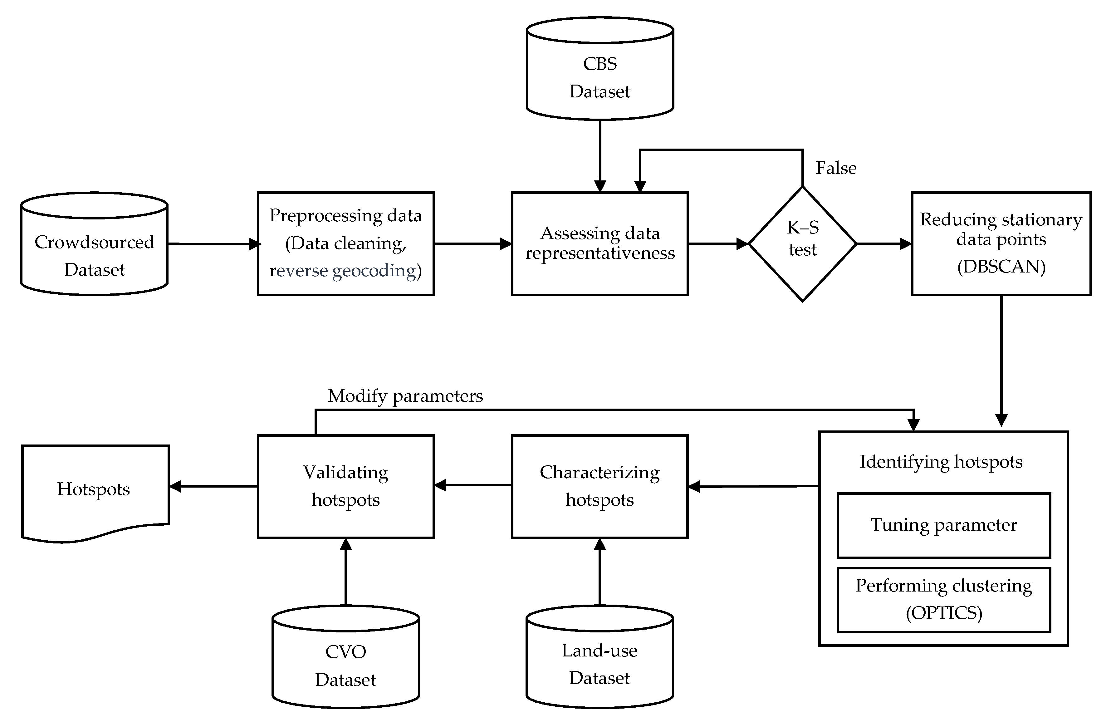
2.3. Methodology
2.3.1. Preprocessing Dataset
2.3.2. Dataset Representativeness
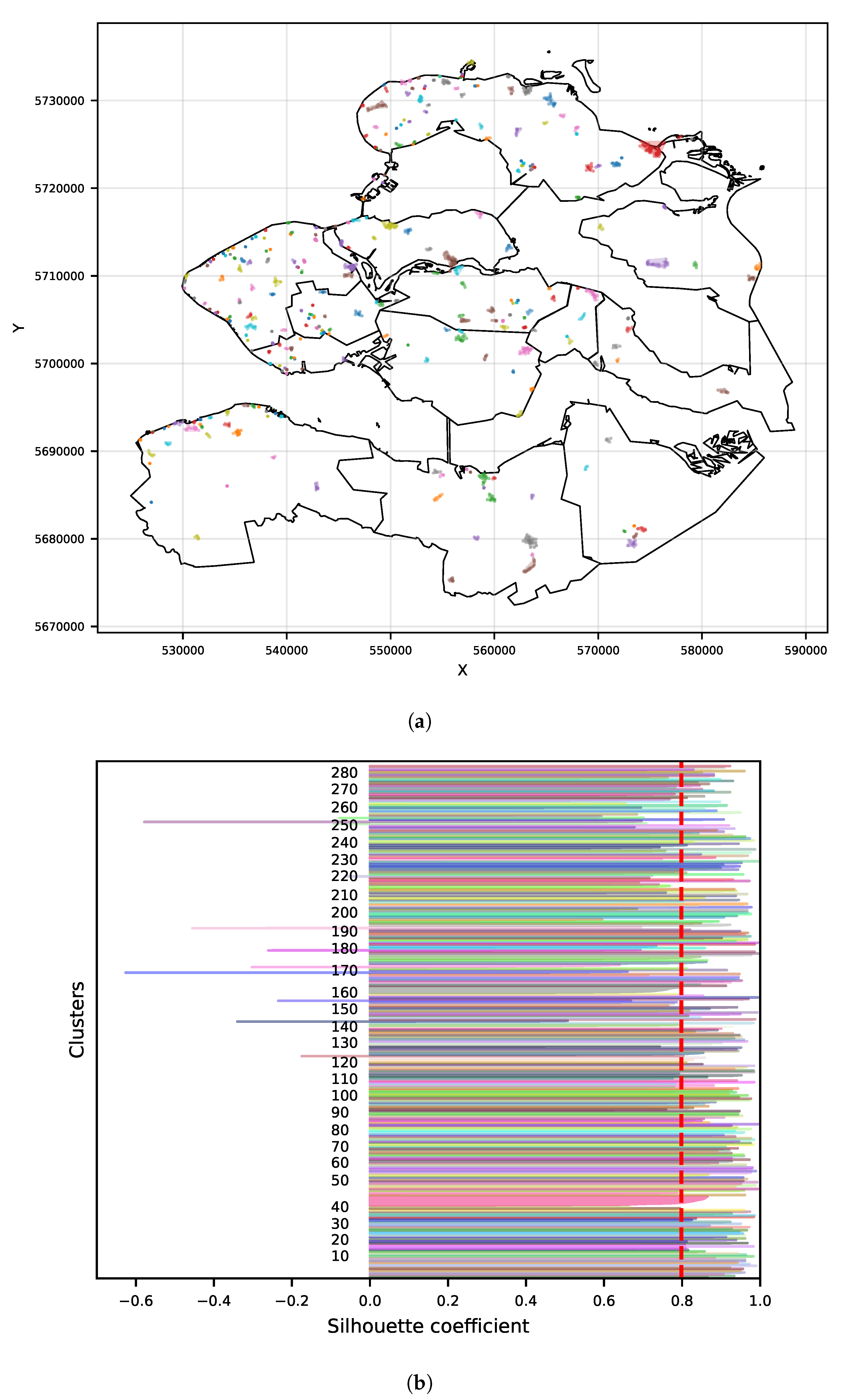
2.3.3. Clustering Analysis
2.3.4. Data-Driven Characterization and Validation
3. Results
3.1. Inbound Travel Analysis for Representativeness
3.2. Experiment
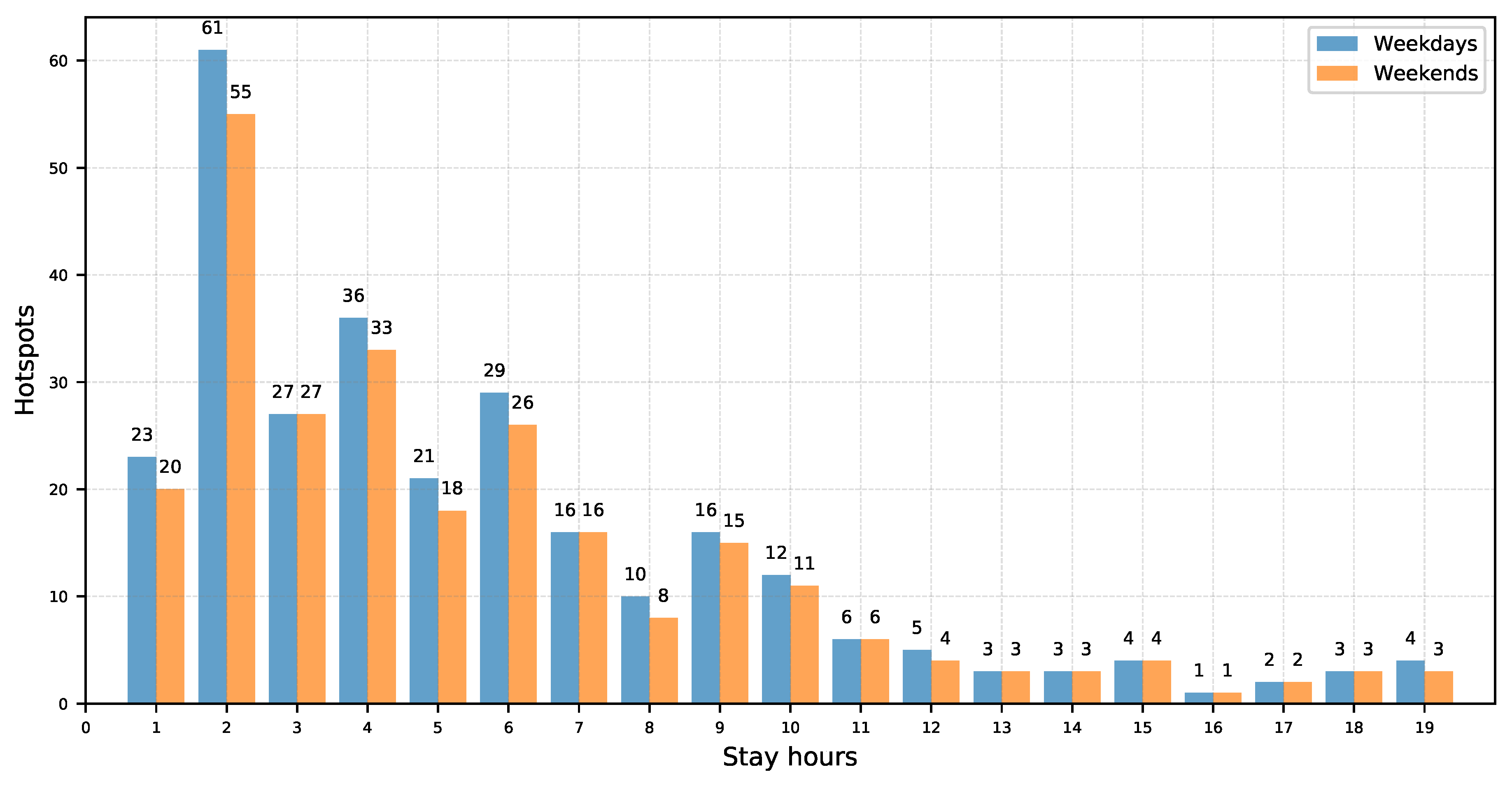
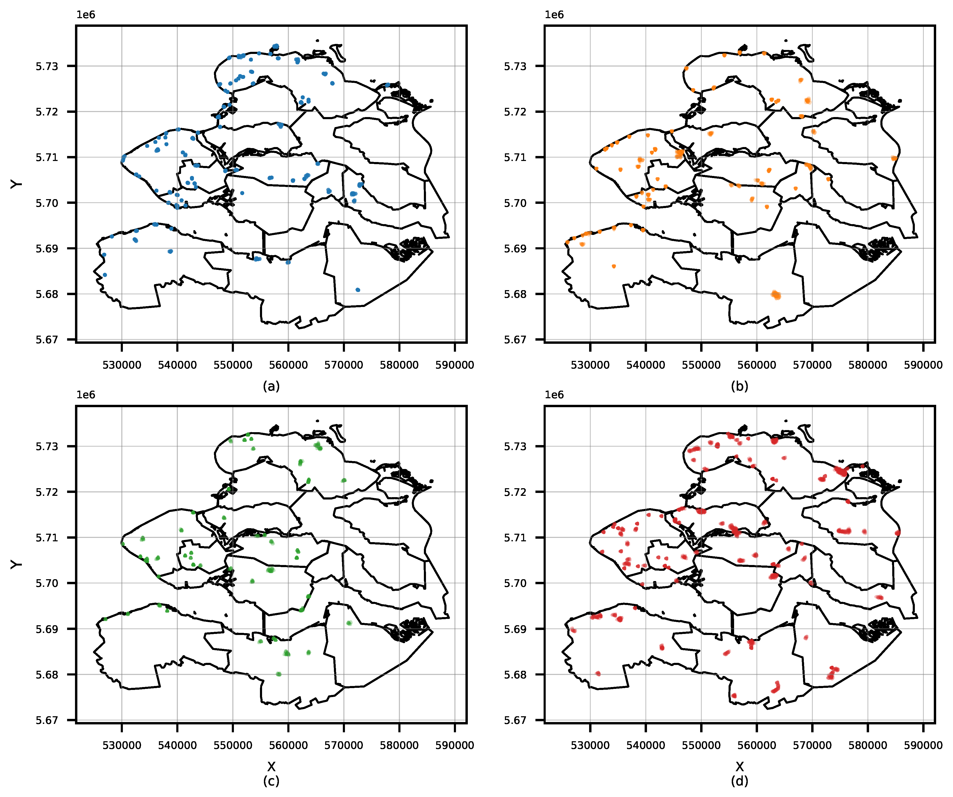
3.3. Tourist Hotspot Data-Driven Insights
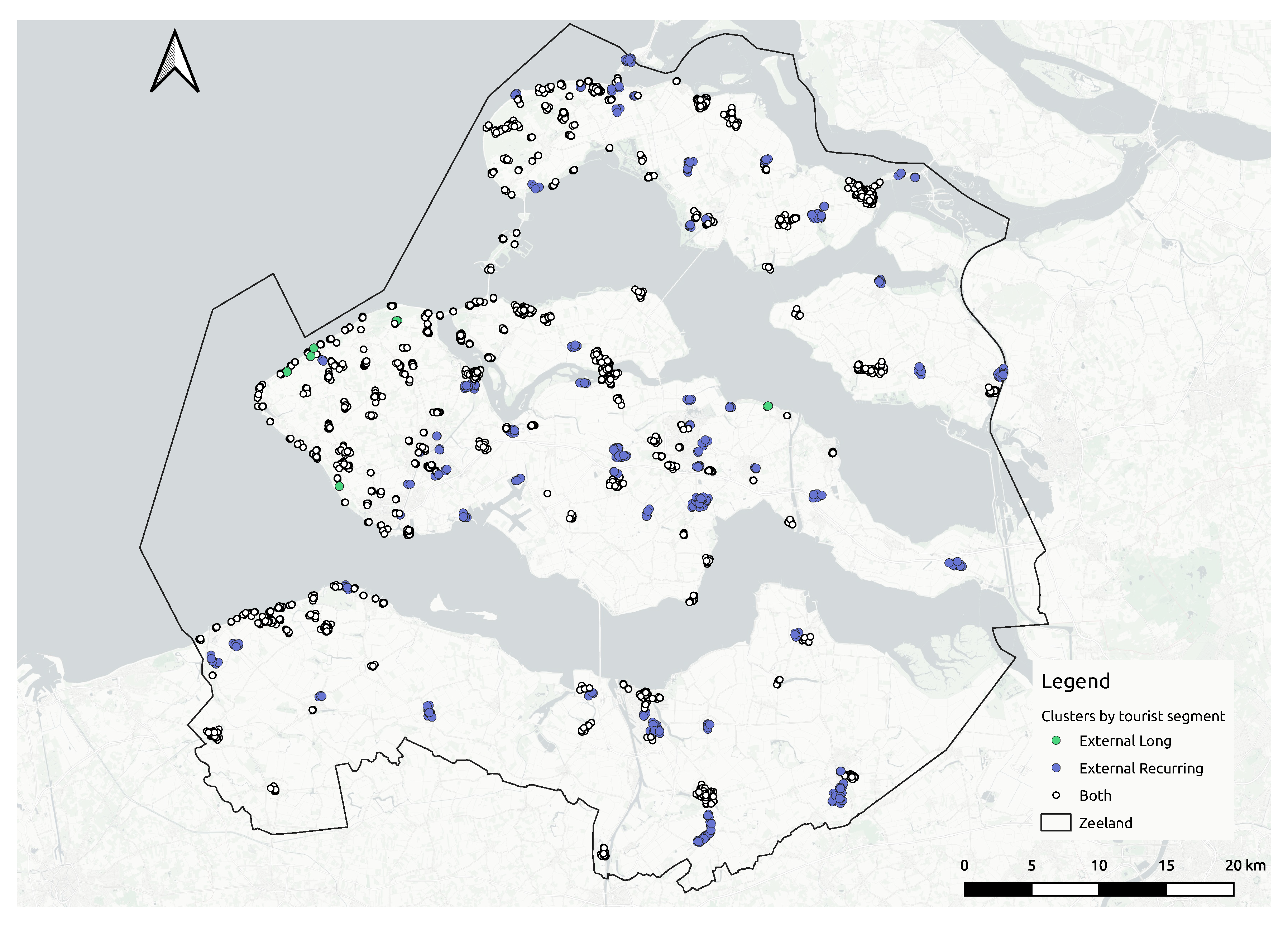
3.4. Crowdsourced Tourist Campaign Insights
4. Discussion
5. Conclusions
Author Contributions
Funding
Acknowledgments
Conflicts of Interest
References
- OECD. OECD Tourism Trends and Policies 2020; OECD Publishing: Paris, France, 2020. [Google Scholar] [CrossRef]
- Tkaczynski, A.; Rundle-Thiele, S.R.; Beaumont, N. Segmentation: A tourism stakeholder view. Tour. Manag. 2009, 30, 169–175. [Google Scholar] [CrossRef]
- Bloom, J.Z. MARKET SEGMENTATION: A Neural Network Application. Ann. Tour. Res. 2005, 32, 93–111. [Google Scholar] [CrossRef]
- Hardy, A.; Hyslop, S.; Booth, K.; Robards, B.; Aryal, J.; Gretzel, U.; Eccleston, R. Tracking tourists’ travel with smartphone-based GPS technology: A methodological discussion. Inf. Technol. Tour. 2017, 17, 255–274. [Google Scholar] [CrossRef]
- Kellner, L.; Egger, R. Tracking tourist spatial-temporal behavior in urban places, a methodological overview and GPS case study. In Information and Communication Technologies in Tourism 2016; Springer: Cham, Switzerland, 2016; pp. 481–494. [Google Scholar]
- Frochot, I. A benefit segmentation of tourists in rural areas: A Scottish perspective. Tour. Manag. 2005, 26, 335–346. [Google Scholar] [CrossRef]
- Hu, B.; Yu, H. Segmentation by craft selection criteria and shopping involvement. Tour. Manag. 2007, 28, 1079–1092. [Google Scholar] [CrossRef]
- Ahas, R.; Aasa, A.; Mark, Ü.; Pae, T.; Kull, A. Seasonal tourism spaces in Estonia: Case study with mobile positioning data. Tour. Manag. 2007, 28, 898–910. [Google Scholar] [CrossRef]
- Rodríguez, J.; Semanjski, I.; Gautama, S.; Van de Weghe, N.; Ochoa, D.; Rodríguez, J.; Semanjski, I.; Gautama, S.; Van de Weghe, N.; Ochoa, D. Unsupervised Hierarchical Clustering Approach for Tourism Market Segmentation Based on Crowdsourced Mobile Phone Data. Sensors 2018, 18, 2972. [Google Scholar] [CrossRef]
- Michail, A.; Gavalas, D. Bucketfood: A Crowdsourcing Platform for Promoting Gastronomic Tourism. In Proceedings of the 2019 IEEE International Conference on Pervasive Computing and Communications Workshops (PerCom Workshops), Kyoto, Japan, 11–15 March 2019; pp. 9–14. [Google Scholar]
- Download Zeeland App—VVV Zeeland. Available online: https://www.vvvzeeland.nl/en/service/zeeland-app/ (accessed on 5 October 2020).
- Ahas, R.; Aasa, A.; Roose, A.; Mark, Ü.; Silm, S. Evaluating passive mobile positioning data for tourism surveys: An Estonian case study. Tour. Manag. 2008, 29, 469–486. [Google Scholar] [CrossRef]
- Yang, C.; Clarke, K.; Shekhar, S.; Tao, C.V. Big Spatiotemporal Data Analytics: A research and innovation frontier. Int. J. Geogr. Inf. Sci. 2019, 34, 1075–1088. [Google Scholar] [CrossRef]
- Wu, C.; Yang, Z.; Xu, Y.; Zhao, Y.; Liu, Y. Human mobility enhances global positioning accuracy for mobile phone localization. IEEE Trans. Parallel Distrib. Syst. 2014, 26, 131–141. [Google Scholar] [CrossRef]
- Spangenberg, T. Development of a mobile toolkit to support research on human mobility behavior using GPS trajectories. Inf. Technol. Tour. 2014, 14, 317–346. [Google Scholar] [CrossRef]
- Semanjski, I.; Bellens, R.; Gautama, S.; Witlox, F. Integrating big data into a sustainable mobility policy 2.0 planning support system. Sustainability 2016, 8, 1142. [Google Scholar] [CrossRef]
- González, M.C.; Hidalgo, C.A.; Barabási, A.L. Understanding individual human mobility patterns. Nature 2008, 453, 779–782. [Google Scholar] [CrossRef] [PubMed]
- Fayyad, U.; Piatetsky-Shapiro, G.; Smyth, P. From data mining to knowledge discovery in databases. AI Mag. 1996, 17, 37–53. [Google Scholar]
- Versichele, M.; de Groote, L.; Claeys Bouuaert, M.; Neutens, T.; Moerman, I.; Van de Weghe, N. Pattern mining in tourist attraction visits through association rule learning on Bluetooth tracking data: A case study of Ghent, Belgium. Tour. Manag. 2014, 44, 67–81. [Google Scholar] [CrossRef]
- Semanjski, I.; Ramachi, M.; Gautama, S. Detection of Points of Interest from Crowdsourced Tourism Data. In Computational Science and Its Applications–ICCSA 2019; Misra, S., Gervasi, O., Murgante, B., Stankova, E., Korkhov, V., Torre, C., Rocha, A.M.A., Taniar, D., Apduhan, B.O., Tarantino, E., Eds.; Springer International Publishing: Cham, Switzerland, 2019; pp. 203–216. [Google Scholar]
- Tang, L.; Gao, J.; Ren, C.; Zhang, X.; Yang, X.; Kan, Z. Detecting and Evaluating Urban Clusters with Spatiotemporal Big Data. Sensors 2019, 19, 461. [Google Scholar] [CrossRef]
- Atiencia, Y.; Cruz, E.; Vaca, C.; Zambrano, L. Spatio-temporal Analysis: Using Instagram Posts to Characterize Urban Point-of-interest. In Proceedings of the 2020 Seventh International Conference on eDemocracy eGovernment (ICEDEG), Buenos Aires, Argentina, 22–24 April 2020; pp. 114–119. [Google Scholar]
- Trendrapport Toerisme, Recreatie en Vrije Tijd. 2019. Available online: https://www.cbs.nl/nl-nl/publicatie/2019/48/trendrapport-toerisme-recreatie-en-vrije-tijd-2019 (accessed on 10 September 2020).
- Centraal Bureau Voor de Statistiek—StatLine—Overnight Accommodation; Guests, Country of Residence, Type, Region. Available online: https://opendata.cbs.nl/#/CBS/en/dataset/82059ENG/table (accessed on 8 July 2020).
- Dataset: CBS Bestand Bodemgebruik. 2015. Available online: https://www.pdok.nl/introductie/-/article/cbs-bestand-bodemgebruik (accessed on 10 September 2020).
- De Customer Journey Cycle in Zeeland. Available online: https://kwaliteit.toerismevlaanderen.be/de-customer-journey-cycle-in-zeeland (accessed on 10 September 2020).
- Rhys, H.I. Machine Learning with R, the Tidyverse, and mlr, 1st ed.; Manning Publications Co.: Shelter Island, NY, USA, 2020; p. 536. [Google Scholar]
- Ester, M.; Kriegel, H.P.; Sander, J.; Xu, X. A density-based algorithm for discovering clusters in large spatial databases with noise. In Proceedings of the Second International Conference on Knowledge Discovery and Data Mining, Portland, OR, USA, 2–4 August 1996; pp. 226–231. [Google Scholar]
- Zhou, A.; Zhou, S.; Cao, J.; Fan, Y.; Hu, Y. Approaches for scaling DBSCAN algorithm to large spatial databases. J. Comput. Sci. Technol. 2000, 15, 509–526. [Google Scholar] [CrossRef]
- Ankerst, M.; Breunig, M.M.; Kriegel, H.P.; Sander, J. OPTICS: Ordering Points to Identify the Clustering Structure. SIGMOD Rec. (ACM Spec. Interest Group Manag. Data) 1999, 28, 49–60. [Google Scholar] [CrossRef]
- Bryant, A.; Cios, K. RNN-DBSCAN: A Density-Based Clustering Algorithm Using Reverse Nearest Neighbor Density Estimates. IEEE Trans. Knowl. Data Eng. 2018, 30, 1109–1121. [Google Scholar] [CrossRef]
- Kisilevich, S.; Mansmann, F.; Keim, D. P-DBSCAN: A density based clustering algorithm for exploration and analysis of attractive areas using collections of geo-tagged photos. In Proceedings of the 1st International Conference and Exhibition on Computing for Geospatial research & Application, Washington, DC, USA, 21–23 June 2010; pp. 1–4. [Google Scholar]
- Schubert, E.; Sander, J.; Ester, M.; Kriegel, H.P.; Xu, X. DBSCAN Revisited, Revisited: Why and How You Should (Still) Use DBSCAN. ACM Trans. Database Syst. 2017, 42. [Google Scholar] [CrossRef]
- Hu, Y.; Gao, S.; Janowicz, K.; Yu, B.; Li, W.; Prasad, S. Extracting and understanding urban areas of interest using geotagged photos. Comput. Environ. Urban Syst. 2015, 54, 240–254. [Google Scholar] [CrossRef]
- Birant, D.; Kut, A. ST-DBSCAN: An algorithm for clustering spatial–temporal data. Data Knowl. Eng. 2007, 60, 208–221. [Google Scholar] [CrossRef]
- Devkota, B.; Miyazaki, H.; Witayangkurn, A.; Kim, S.M. Using Volunteered Geographic Information and Nighttime Light Remote Sensing Data to Identify Tourism Areas of Interest. Sustainability 2019, 11, 4718. [Google Scholar] [CrossRef]
- Vu, H.Q.; Li, G.; Law, R.; Ye, B.H. Exploring the travel behaviors of inbound tourists to Hong Kong using geotagged photos. Tour. Manag. 2015, 46, 222–232. [Google Scholar] [CrossRef]
- Rousseeuw, P.J. Silhouettes: A graphical aid to the interpretation and validation of cluster analysis. J. Comput. Appl. Math. 1987, 20, 53–65. [Google Scholar] [CrossRef]
- Dubes, R.; Jain, A.K. Validity studies in clustering methodologies. Pattern Recognit. 1979, 11, 235–254. [Google Scholar] [CrossRef]
- Rodríguez Echeverría, J.; Gautama, S.; Van de Weghe, N.; Ochoa, D.; Ortiz Jaramillo, B. Efficient use of geographical information systems for improving transport mode classification. In DATA ANALYTICS 2018: The Seventh International Conference on Data Analytics, Athens, Greece, 18–22 November 2018; Bhulai, S., Kardaras, D., Semanjski, I., Eds.; International Academy, Research and Industry Association (IARIA): Wilmington, DE, USA, 2018; pp. 130–135. [Google Scholar]
- Filip Biljecki, H.L.; van Oosterom, P. Transportation Mode-based Segmentation and Classification of Movement Trajectories. Int. J. Geogr. Inf. Sci. 2013, 27, 385–407. [Google Scholar] [CrossRef]
- Gong, H.; Chen, C.; Bialostozky, E.; Lawson, C.T. A GPS/GIS method for travel mode detection in New York City. Comput. Environ. Urban Syst. 2012, 36, 131–139. [Google Scholar] [CrossRef]
- Basiri, A.; Haklay, M.; Foody, G.; Mooney, P. Crowdsourced geospatial data quality: Challenges and future directions. Int. J. Geogr. Inf. Sci. 2019, 33, 1588–1593. [Google Scholar] [CrossRef]
- Leao, S.Z.; Lieske, S.N.; Pettit, C.J. Validating crowdsourced bicycling mobility data for supporting city planning. Transp. Lett. 2019, 11, 486–497. [Google Scholar] [CrossRef]
- Bubalo, M.; van Zanten, B.T.; Verburg, P.H. Crowdsourcing geo-information on landscape perceptions and preferences: A review. Landsc. Urban Plan. 2019, 184, 101–111. [Google Scholar] [CrossRef]
- Ghose, A.; Ipeirotis, P.G.; Li, B. Designing ranking systems for hotels on travel search engines by mining user-generated and crowdsourced content. Mark. Sci. 2012, 31, 493–520. [Google Scholar] [CrossRef]
- Yuan, Y.; Wei, G.; Lu, Y. Evaluating gender representativeness of location-based social media: A case study of Weibo. Ann. GIS 2018, 24, 163–176. [Google Scholar] [CrossRef]
- Omvang Toerisme in Zeeland 2018—Projectenportfolio. Available online: https://www.projectenportfolio.nl/wiki/index.php/KCKT_Publication_PR_00006 (accessed on 8 July 2020).
- Weinberg, J.D.; Freese, J.; McElhattan, D. Comparing Data Characteristics and Results of an Online Factorial Survey between a Population-Based and a Crowdsource-Recruited Sample. Sociol. Sci. 2014, 1, 292–310. [Google Scholar] [CrossRef]
- Van Gheluwe, C.; Lopez, A.J.; Gautama, S. Error sources in the analysis of crowdsourced spatial tracking data. In Proceedings of the 2019 IEEE International Conference on Pervasive Computing and Communications Workshops (PerCom Workshops), Kyoto, Japan, 11–15 March 2019; pp. 183–188. [Google Scholar]


| Variable | Acronym | Description |
|---|---|---|
| User’s ID | userid | Unique identifier assigned to the device during the installation of the Zeeland app. A user is linked with only one device. |
| Start time | start | Timestamp when the trip segment started. |
| End time | end | Timestamp when the trip segment ended. |
| Mode of transportation | mode | Mode of transportation used in the trip segment. |
| Distance | distance | Distance traveled between the trip segment’s starting and ending points measured in meters. |
| Waypoints | waypoints | Trajectory of geographic locations (latitude, longitude) followed from the trip segment’s starting until ending point. Additionally, every geography location contains the timestamp when the measure was gathered. |
| Duration | duration | Duration of the trip segment measured in seconds. |
| Field | Acronym | Description |
|---|---|---|
| Property’s ID | BG2015 | Unique identifier of a property. |
| Land-use level 1 | Hoofdgroep | Level-1 description of the land-use of a property. It represents the main land-use. |
| Land-use level 2 | Omschrijvi | Level-2 description of the land-use of a property. |
| Length of the property | Shape_Leng | Representative of the length of the geometry’s property. |
| Area of the property | Shape_Area | Representative of the length of the geometry’s property. |
| Rank | Purpose | Tourists |
|---|---|---|
| 1 | Visit to the beach | 82% |
| 2 | Eating out | 70% |
| 3 | Take walks | 66% |
| 4 | Fun shopping | 37% |
| 5 | Swimming | 35% |
| 6 | Bike rides | 35% |
| 7 | Visit to nature reserve | 29% |
| 8 | Visits to interesting buildings | 29% |
| 9 | Sunbathing | 15% |
| 10 | Visit to the museum | 9% |
| Variable | Acronym | Description |
|---|---|---|
| User’s ID | userid | Unique identifier of the user. |
| Destination location | destiny | Geographic location (latitude, longitude) of the trip’s destination. |
| Municipality origin | municipality_o | Municipality where the trip started. In case the trip started out from the area is set up as empty. |
| Municipality destination | municipality_d | Municipality where the trip destination is located. |
| Arrival time | end | Timestamp when the trip ended. |
| Weekend | weekend | Represents whether or not the trip occurred during a weekend. |
| Stay time | stay | Represents how long time (hours) exists between the arrival time and the starting time of the next registered trip. |
| Tourist segment | segment | Represents the user tourist profile: External long, External recurring. |
| Variable | Acronym | Description |
|---|---|---|
| Longitude | longitude | Represents the longitude component from the geographic location in UTM coordinate system. |
| Latitude | latitude | Represents the latitude component from the geographic location in UTM coordinate system. |
| Level 1 | Area (%) | Level 2 | Hotspots |
|---|---|---|---|
| Agriculture | 36.85 | Other agricultural use | 17 |
| Airport | 0.01 | Airport | 1 |
| Built | 2.21 | Allotment | 1 |
| Residential area | 68 | ||
| Retail and catering | 26 | ||
| Socio-cultural provision | 3 | ||
| Business premises | 1.02 | Business premises | 23 |
| Dry natural terrain | 1.04 | Dry natural terrain | 49 |
| Forest | 1.11 | Forest | 3 |
| Highway | 1.78 | Highway | 24 |
| Recreation | 1.31 | Day recreation area | 9 |
| Leisure recreation | 36 | ||
| Park and public garden | 3 | ||
| Sports field | 5 | ||
| Semi-built | 1.01 | Building site | 4 |
| Cemetery | 1 | ||
| Semi-paved other terrain | 13 | ||
| Water | 49.77 | Estuary | 1 |
| Wet natural terrain | 1.86 | Wet natural terrain | 1 |
Publisher’s Note: MDPI stays neutral with regard to jurisdictional claims in published maps and institutional affiliations. |
© 2020 by the authors. Licensee MDPI, Basel, Switzerland. This article is an open access article distributed under the terms and conditions of the Creative Commons Attribution (CC BY) license (http://creativecommons.org/licenses/by/4.0/).
Share and Cite
Rodríguez-Echeverría, J.; Semanjski, I.; Van Gheluwe, C.; Ochoa, D.; IJben, H.; Gautama, S. Density-Based Spatial Clustering and Ordering Points Approach for Characterizations of Tourist Behaviour. ISPRS Int. J. Geo-Inf. 2020, 9, 686. https://doi.org/10.3390/ijgi9110686
Rodríguez-Echeverría J, Semanjski I, Van Gheluwe C, Ochoa D, IJben H, Gautama S. Density-Based Spatial Clustering and Ordering Points Approach for Characterizations of Tourist Behaviour. ISPRS International Journal of Geo-Information. 2020; 9(11):686. https://doi.org/10.3390/ijgi9110686
Chicago/Turabian StyleRodríguez-Echeverría, Jorge, Ivana Semanjski, Casper Van Gheluwe, Daniel Ochoa, Harm IJben, and Sidharta Gautama. 2020. "Density-Based Spatial Clustering and Ordering Points Approach for Characterizations of Tourist Behaviour" ISPRS International Journal of Geo-Information 9, no. 11: 686. https://doi.org/10.3390/ijgi9110686
APA StyleRodríguez-Echeverría, J., Semanjski, I., Van Gheluwe, C., Ochoa, D., IJben, H., & Gautama, S. (2020). Density-Based Spatial Clustering and Ordering Points Approach for Characterizations of Tourist Behaviour. ISPRS International Journal of Geo-Information, 9(11), 686. https://doi.org/10.3390/ijgi9110686