1. Introduction
Finding the fastest path in a road network is a common task that needs to be solved in various applications such as transportation, route planning, or disaster risk managing (see, for example, [
1,
2,
3,
4]).
For routing applications, OpenStreetMap (OSM) road data are frequently used. The main reason for this is that OSM is one of the best-known volunteered geographic information projects and features free data available worldwide and real-time updates [
5,
6]. However, OSM data have some disadvantages concerning the road network data quality due to the participatory character of the OSM project [
1,
3,
4,
6,
7]. The completeness varies significantly between the different countries worldwide, both in terms of the feature completeness and the attribute completeness [
7].
Most routing applications ask for the link travel time as a parameter since information about the road network is crucial. According to Stanojevic et al. [
8], the link travel time is the average time that it takes a vehicle to pass a road segment. The average speed information together with the length of a road segment can be used to calculate the respective road segment’s link travel time. We consider a road segment similar to an edge of the road network in a topological representation of the network.
In the OSM road network, neither the link travel time nor the average speed information, necessary for routing applications, is directly available. Alternatively, the maximum speed information for a road segment is often used if provided. However, 92.2% of all road kilometers worldwide in the 2019 OSM road network lack the maximum speed information [
9]. Solely approximately ten countries have more than 40% of the road networks kilometers tagged with the maximum speed information. The completeness of the maximum speed information is higher in urban areas than in rural areas [
9,
10,
11,
12]. If the maximum speed information is available, this information sometimes is multiplied with a factor to approximate the average speed as input for routing applications. If the maximum speed information is missing, fixed speed information for each road class is assumed [
5]. The latter creates discontinuous jumps at transitions between different road classes, which causes adverse effects for routing applications. To avoid these jumps, we recently proposed a Fuzzy Framework for Speed Estimation (Fuzzy-FSE) to estimate the average speed on rural roads relying on multiple input features of the OSM road network [
9]. Although the Fuzzy-FSE performs well, its prediction accuracy depends highly on the rules’ individual design and the underlying expert knowledge.
The average speed information varies between rural and urban areas since different conditions have to be considered. In rural areas, the average speed is mainly influenced by the road quality, the road slope, or the road width. These parameters can all be deduced from OSM road data. Approximating the average speed of roads in urban areas would require information such as temporal aspects of traffic. This information cannot be deduced from OSM road data.
1.1. Motivation and Objective
Our study is motivated by the aspect that in the OSM road network data, 92.2% of all road kilometers worldwide have missing maximum speed information, especially in rural areas. The OSM road network also does not provide the average speed information. Moreover, the Fuzzy-FSE, as the only available approach to predict for average speed prediction based on OSM road network data, needs much domain-knowledge. As a result, the Fuzzy-FSE is not generally applicable to different regional datasets.
Therefore, we aim at imputing the OSM road network data with average speed information by applying machine learning (ML) approaches solely on OSM road network input data. Our objective is to provide a more generalized data-driven approach to predict this speed information that currently does not exist. The predicted speed information, then, can be used in routing applications. This intention naturally leads to a general but intriguing question:
Can purely data-driven ML approaches predict the average speed of rural road segments when trained on generic inhomogeneous OSM road network data? To address this overall question, we develop a ML estimation framework following a typical ML processing pipeline and investigate the underlying input data. Furthermore, we use the same datasets as Guth et al. [
9] to compare our ML estimation framework’s predictions and the results derived by the Fuzzy-FSE. The reference data included in these datasets are average speed values extracted from the Google Directions API (GD-API).
In contrast to the Fuzzy-FSE approach, we also investigate the ability of the ML estimation framework to link the OSM road network input data to GD-API data without further domain-knowledge. The average speed reference data acquired from GD-API are characterized by speed values with a large variance per road class (see
Section 2.1) and cause heterogeneous datasets. These heterogeneous datasets occur even within individual regions, which is a challenging task for the ML estimation framework’s applicability. Moreover, we begin to evaluate the proposed ML estimation framework’s possible generalization capacity by combining different regional datasets.
Concerning the mentioned aspects and challenges, we summarize our primary objective as follows: we aim to design an estimation framework, including existing ML approaches, that yields a robust average speed prediction against various variabilities in the OSM road network input data. This estimation framework needs to handle a limited number of heterogenous training data for the ML approaches. We freely provide the implementation of our entire methodological workflow with an exemplary dataset on GitHub [
13]. The main contributions linked to the study’s objective are summarized in the following:
the development of an estimation framework for average speed in rural road networks inspired by a typical ML pipeline as a methodology;
a detailed investigation and evaluation of the potential of the estimation framework based on the heterogenous OSM road network input features to predict average speed;
the selection of the most important features for the estimation of the average speed based on the ML models;
a novel approach to apply Self-Organizing Maps (SOMs) as a unsupervised ML approach to generate new features;
an application of the methodology on two distinct study regions in Chile and Australia and the presentation of the respective results;
the comparison of the regression performance of the estimation framework with the Fuzzy-FSE predictions.
In
Section 1.2, the research background is briefly stated. We present the different levels of the estimation framework for average speed in road networks in
Section 2. This section includes the proposed methodological procedure with the description of the three different datasets, the preprocessing steps and the dataset splittings, the feature level with generating additional features, and the model level. The regression results are presented in
Section 3. Subsequently, we assess and evaluate the performance of the estimation framework (
Section 4). In
Section 5, the presented study is concluded, combined with an outlook of further studies.
1.2. Research Background
In the following, we briefly summarize the research background. As our study focuses on estimating average speed information based on OSM road network data, we first take a glance at possibilities to calculate average speed values, the link travel times, with OSM data. Furthermore, we present a ML application using OSM data to solve different classification tasks.
There exist numerous routing applications based on OSM road network data. Examples are the OpenRouteService [
14], the Open Source Routing Machine (OSRM) [
5], the OpenTripPlanner [
15], and YOURS [
16]. All of these examples have to overcome the challenge of estimating average speed to derive link travel times. The OSRM, the OpenTripPlanner, and YOURS use the information from the OSM tag
maxspeed to calculate link travel time if this tag is available. If the maximum speed information is missing, predefined speed limits for each country are applied [
17]. Details on these surrogate information sources can be found in the OSM Wiki. Other tag information such as the road type and the number of lanes are used to derive fixed speed values for each road class. The OpenRouteService seems to be based on a more complex travel time calculation as it features additional information like the slope or type of a route. However, the exact calculation is not transparent.
In the research community, few studies exist that address link travel time in the OSM road network. Stanojevic et al. [
8] use origin-destination and timestamp information generated by a taxi fleet and OSM road data to calculate link travel times. Their estimation proves to have 60% lower errors in urban regions than OSRM. Further, Steiger et al. [
18] include real-time traffic data into the OpenRouteService to improve the estimation in urban regions. Generally, most research studies focus on the estimation of travel time in urban regions.
Concerning the combination of ML approaches and OSM data, some studies have been conducted, mainly dealing with supervised classification tasks. For example, OSM data and ML approaches are used for semantic labeling of earth observation images [
19]. Deep neural networks are applied to OSM data to leverage OSM data for semantic labeling of aerial and satellite images. Schultz et al. [
20] use sixty tags in OSM data to allocate a Corine Land Cover level 2 land use classification. The potential for rapid land use and land cover mapping based on time-series Landsat satellite images and OSM data is evaluated in Johnson and Iizuka [
21]. Besides, ML approaches are used to solve classification tasks addressing the OSM data quality. For example, Jilani et al. [
22] focus on assessing OSM data quality while Kaur and Singh [
23] improve the OSM data quality. Jilani et al. [
22] address the semantic accuracy of OSM street network data by training a ML model to learn the geometry and topology of distinct street classes. Subsequently, the trained model is applied to correct the semantic class of the streets. Kaur and Singh [
23] use a ML model with OSM attributes such as road length to improve the OSM data quality by detecting and correcting errors within the OSM data. In this case, they consider missing or incorrect attributes of nodes and ways in the OSM network as errors. In a further study, the extrapolation of missing street names is addressed with ML approaches that can learn the OSM road network’s topology and semantic [
24]. A few studies focus on the correction of specific OSM tags with supervised ML techniques, the detection of errors in OSM, and generally improving the OSM data quality in terms of attribute accuracy and consistency (see, for example, [
25,
26,
27]).
ML approaches are not yet applied for regression tasks or even for estimating average speed information, respectively, travel times. Only one approach exists, which can be used to estimate the average speed of rural roads with only OSM road network data [
9]. This approach relies on domain knowledge and is called a Fuzzy Framework for Speed Estimation (Fuzzy-FSE). The Fuzzy-FSE is not categorized as a solely data-driven approach, in contrast to ML approaches. It relies on fuzzy control with the input parameters road class, road slope, road surface, and link length originated from the OSM road network and optionally, a freely available digital elevation model (DEM). A rule and knowledge base describing the output member functions and a Fuzzy Control System calculating the output average speeds are the two parts of the Fuzzy-FSE.
2. Datasets and Methodology in the Estimation Framework
In general, we can apply several approaches when using machine learning (ML) for regression tasks (see, for example, [
28,
29,
30]). The selected approaches depend on the available reference data and the quality or amount of the available data. For the underlying regression task of estimating the average speed for distinct road segments with solely OSM road network data, we rely on an estimation framework to condense suitable ML approaches (see
Figure 1). This framework structures the task in four levels by following a typical ML pipeline and embraces our study’s methodology. (1) In the dataset level, we describe the used dataset and, more specifically, the OSM input data and the corresponding reference data. (2) The data level contains the preprocessing and the dataset splitting necessary for the ML models’ training and evaluation. (3) At the feature level, we apply unsupervised dimensionality reduction, unsupervised clustering, and feature selection. (4) The model level contains supervised learning, model selection, the optimization of the hyperparameters, and the model evaluation metrics. The code of the estimation framework for an exemplary dataset is freely available on GitHub [
13]. Note that due to copyrights, we cannot publish the original reference data. Therefore, we generated simulated reference data (for details see [
13]).
We utilize the mathematical notation according to Chapelle et al. [
31], where
denotes a set of
N input datapoints
for all
. Every datapoint
, in our case, every road segment, consists of
M input features (see
Table 1). For the regression of the average speed values, the target values of the reference data are continuous meaning
. As reference data, average speed values are available for selected input datapoints. We apply supervised and unsupervised learning models on all three datasets in the proposed estimation framework (see
Figure 1). Further, we apply unsupervised learning approaches on the feature level and adding the generated features to the input data. For the supervised learning approaches,
with
are the average speed values of the datapoints
(road segments), and the training set is given as pairs
. From now on, we refer to the combination of input features and desired output data as a datapoint. The applied variable naming conventions are summarized in
Table A1.
2.1. Datasets
For a reliable estimation of the average speed in road networks with ML approaches, several datasets are required to train and evaluate the selected models. We rely on datasets that include mainly OSM road network data due to their free and worldwide availability. The datasets represent the first level of the estimation framework, as shown in
Figure 1. In this study, we consider three datasets: the BM dataset (Chile), the NNSW dataset (Australia), and the combined dataset (Chile and Australia). Each of these datasets includes the condensed OSM road network data and average speed values. The latter is extracted from the Google Directions API (GD-API) and serves as reference data (or ground truth data).
The first dataset consists of OSM road network data for the BioBío, Ñuble, and Maule (BM) regions in central Chile. The Ñuble region is a relatively new region that was created in 2018 by splitting the former BioBío region into two separate regions. Thus, the BM dataset is the same as in [
9], even though it now consists of three regions. The second dataset includes OSM road network data for the statistical divisions Mid-North Coast, Richmond-Tweed, and Northern in the north of New South Wales in Australia (NNSW). A third, combined, dataset is formed by merging both datasets. The study regions in Chile and Australia are comparable in size but are at different development stages. Guth et al. [
9] present the characteristics of these regions in a more detailed manner. In the following, we briefly summarize the main characteristics and differences between the three datasets.
In contrast to Chile, Australia’s road infrastructure is developed further and contains a wide range of paved and high-level roads. In Chile, many unpaved roads exist where the average speed is low compared to the same road classes in more developed countries concerning the road infrastructure. Both regions feature large rural areas that are sparsely populated. Part of the study region in Chile is located in the Andes so that the range of slopes for the BM dataset is vast compared to the less mountainous NNSW region.
The regions are chosen because they demonstrate the applicability of the data-driven estimation framework in geographically diverse regions. Furthermore, the OSM road network data’s quality and availability differ in both regions. The OSM road network dataset for NNSW is more complete and contains further additional information than the BM dataset. Note that we compare the ML estimated average speed values with the purely knowledge-based Fuzzy estimated speed values of Guth et al. [
9]. Nevertheless, the generalization capabilities are demonstrated by applying the framework to the combined dataset.
The dataset is partitioned in input data and reference data as the desired output for the applicability of the ML models. The input data and the reference data, respectively, and the target variable are explained in the following section.
2.1.1. OSM Road Network Data as Input Features
The OSM road data as a road network are structured hierarchically in
motorway, trunk, primary, secondary, tertiary, unclassified with their respective link roads
motorway_link, trunk_link, primary_link, secondary_link, tertiary_link. Similar to Guth et al. [
9], further existing road classes are not considered in this estimation framework. Details on the hierarchy of road classes in the OSM road network are presented in [
4,
32].
To estimate average speed in road networks with ML approaches, each road segment of the OSM road network dataset is regarded as one datapoint. This road segment’s respective available attributes are the input features of the estimation task and are listed in
Table 1. In this study, we rely on the input features
class_id, end_latitude, end_longitude, length, region_id, sinuosity, slope_1, slope_2, start_latitude, start_longitude, support_points_km, surface_id. Besides, we extract our own input features by applying, for example, unsupervised clustering on the feature level of the estimation framework (third level in
Figure 1).
Table 2 provides an overview of the OSM road network data of all three datasets. The distribution of the available road data over all road classes is represented. The surface information in OSM is classified into the two main categories,
paved and
unpaved. In some cases, more detailed surface information is available such as
asphalt. If available, we use the more detailed surface information in the estimation framework. In the NNSW dataset, the attribute
surface has the following tags:
unpaved (34.52% of road kilometers),
asphalt (22.09% of road kilometers),
no information (21.42% of road kilometers),
paved (8.59% of road kilometers),
gravel (7.60% of road kilometers),
dirt (2.86% of road kilometers),
concrete (1.09% of road kilometers),
ground (0.86% of road kilometers) and
compacted (0.72% of road kilometers). All other values are featured in less than 0.1% of road kilometers in NNSW.
In the BM dataset, the attribute surface has the following tags: unpaved
(55.15% of road kilometers), paved (17.16% of road kilometers), no information (16.93% of road kilometers), asphalt (8.69% of road kilometers), gravel (1.26% of road kilometers), concrete (0.31% of road kilometers), ground (0.19% of road kilometers) and dirt (0.13% of road kilometers). All other values are featured in less than 0.1% of road kilometers in the BM regions.
Since the combined dataset is a merge of both regional datasets, each attribute’s amounts over all road classes are proportional to the BM and the NNSW dataset.
2.1.2. Average Speed Information as Reference Data and Target Variable
As target variables and, therefore, reference data, we rely on average speed information extracted by the GD-API. The GD-API requires two locations as input points and provides the distance in meters between these locations, the travel time in seconds at a given time, and the coordinates of the points on the road closest to the input point coordinates. Google Maps and its underlying road and traffic information are the basis of the GD-API service. Although many challenges occur when fusioning Google Maps data and OSM road network data (see, for example, [
9,
34]), the GD-API extracted average speed information represents the best choice of reference data in this context. Thus, we assume the GD-API generated average speed values of the respective road segment as reference data despite possible small discrepancies. The average speed distribution for each road class of the reference data is illustrated in
Figure 2. The average speed values vary widely within each road class. The occurring variance of the reference data is a challenging task for the ML regression. We assume that the smaller the range of the average speed values are, the better the ML models can link the OSM road network data such as the
class_id or the
surface_id with the respective average speed values.
2.2. Data Level
The data level is the second level of the presented estimation framework. It is divided into preprocessing (
Section 2.2.1) and dataset splitting (
Section 2.2.2).
2.2.1. Preprocessing
After analyzing the datapoints of all three datasets individually, we excluded any road segment that has one of the following characteristics: the distance between either the start or the end points on the road segment in the input and reference data is larger than 50 m, the lengths of the road segment in input and reference data differ in more than 20%, the road segment is shorter than 600 m, as well as when the GD-API request has returned an error or an empty set. Except for the 600 m threshold, these safeguards are applied to eliminate incorrect data and inconsistencies between the two data sources. Outlier detection is performed in analogy to Guth et al. [
9] to ensure compatibility. Note that we remove the road segments shorter than 600 m since for shorter road segments, the average speed values extracted by GD-API are less accurate due to conversions of the travel time in seconds (for details, see Section 3.3 in Guth et al. [
9]). The raw OSM road network data are minimized to the tags and input features described in
Section 2.1.1.
As a last preprocessing step, we standardize the datasets (standard-scaler, [
35]) to ensure the independence of the ML model training from the scale of the input features.
2.2.2. Dataset Splitting
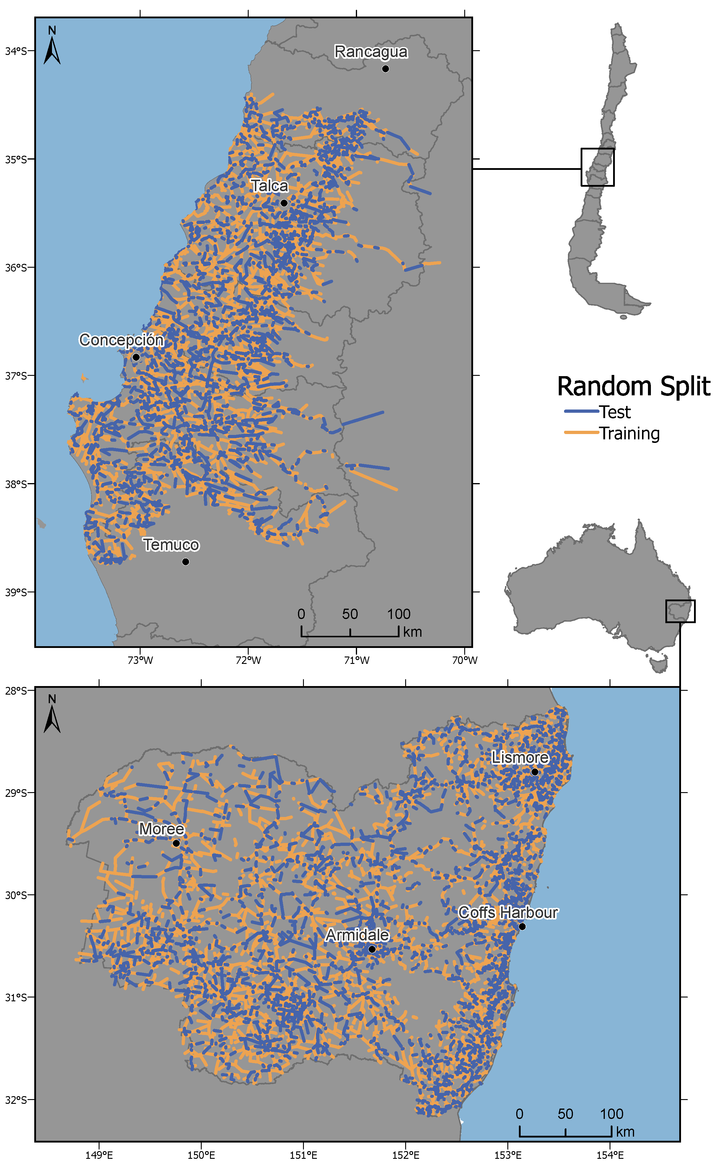
The three datasets (BM, NNSW, and the combination of both) are shuffled, and each dataset is split afterwards randomly into two subsets to evaluate our selected ML models’ generalization ability. The two arising subsets are the training and the test subset.
Each training subset contains 70% of the full dataset’s datapoints, while each test subset consists of the remaining 30% datapoints (see
Figure 3).
Figure 4 visualizes the spatial distribution of the random split for the BM dataset and the NNSW dataset.
Figure 3 shows the corresponding distribution of the target values (average speed) for the training and the test subsets of all datasets.
Table 3 shows the distribution of counts between the three datasets.
2.3. Feature Level
In the presented estimation framework (see
Figure 1), the feature level represents the third level and consists of unsupervised dimensionality reduction, unsupervised clustering, and feature selection. We focus on two approaches: we extract new features with the Principal Component Analysis (PCA, [
36]) as a standard approach of unsupervised dimensionality reduction and we generate new features with a novel approach applying Self-Organizing Maps (SOMs, [
37,
38,
39]) as unsupervised clustering.
The PCA transforms the OSM road network input data (see
Table 1) orthogonally according to the variance along newly found axes, the principal components. The largest variance characterizes the first component. The variance of the subsequent components decreases. Hence, the first few of the principal components contain most of dataset’s variance. We rely on two PCA components, which are computed from the OSM road network input data with the scikit-learn Python package [
35].
Clustering approaches group datapoints based on a predefined similarity metric, mostly in an unsupervised manner. We apply SOMs, which are a shallow type of artificial neural network [
37] consisting of an input layer and a two-dimensional (2D) grid as an output layer. The two layers are fully connected, and the neurons on the output grid are linked to each other based on a neighborhood relationship. This neighborhood relationship determines that any change of one output neuron affects all neurons in its neighborhood on the output grid. In addition to the comprehensible visualization of the SOM’s 2D output grid, the SOM is unsusceptible to overfitting of the training dataset.
To generate new features with the SOM, we apply the unsupervised SOM clustering of Riese et al. [
39] using the SuSi Python package [
40]. Kohonen [
37], Riese and Keller [
38] and Riese et al. [
39] describe the unsupervised SOM algorithm in detail. The unsupervised SOM clusters the OSM road network data in a 2D output grid by finding the best matching unit (BMU) based on the Euclidean distance. Subsequently, we pick the row and column values of the BMU position as new features. These features are named
som_bmu_column and
som_bmu_row. Besides, we partition the SOM output clusters by a k-means clustering with the number of unique
class_id values as the number of clusters. Finally, two additional features are generated,
som_column_clustered and
som_row_clustered, as the k-means cluster centers’ position. The SOM-generated features do not necessarily correspond with a real-world characteristic of the underlying data. Nevertheless, such a correspondence often exists. Besides, the SOM-generated features encompass a more condensed and generalized representation of a given segment, just like the PCA’s principal components. For a more in-depth analysis and examples for the generated features, see
Section 4.1.
In total, we obtain different combinations of input features for the ML models and each dataset.
Table 4 summarizes the combinations that we apply as input features for the ML models and further discuss in this study.
2.4. Model Level
We select appropriate ML models to estimate the average speed information on rather heterogeneous input features extracted from OSM road network data. These ML models are included in the estimation framework (see
Figure 1, fourth level). The selected models (see
Table A2) range from a simple Linear regression model (Linear) to more sophisticated regression models such as Support Vector Machines (SVM), Adaptive Boosting (AdaBoost), Bagging regression (Bagging), Gradient Boosting (GB), Extremely Randomized Trees (ET), Ridge regression (Ridge) up to models capable of unsupervised as well as supervised learning like Self-Organizing Maps (SOM) (see, for example, [
28]). Most of the selected supervised regression models are associated with tree-based regression based on decision trees (DTs). They consist of a root and a leave node that are linked by branches. Generally, DT split the training dataset at every branch and generate subsets depending on, for example, the OSM road network input features [
41].
While the SOM on the feature level (see
Section 2.1) is applied in an unsupervised manner, the SOM on the model level serves as a supervised regression model. In this specific case, the supervised SOM weights are characterized by the same dimension as the target variable, the average speed values. These weights are one-dimensional. Eventually, the combination of the unsupervised and the supervised SOM is able to fulfill the supervised regression task due to a selection of the BMU for each road segment and linkage of the selected BMU to a specific estimation (for a detailed description, see, for example, [
39]).
The hyperparameters of the respective regression models are summarized in
Table A2. The hyperparameters are chosen before the training phase of a ML model. We obtain the hyperparameters by a Basic grid search in conjunction with some manual tuning. During the training phase, the ML models of the estimation framework are trained on the three different training datasets which arise from the three datasets: BM dataset, NNSM dataset, and the combined dataset. The training phase’s objective is to link the OSM road network input features plus the combination with different newly generated features (see
Section 2.3) to the average speed values. As mentioned before, all ML models, except for the SOM regressor, perform the training phase solely supervised.
During the subsequent test phase, the estimation framework’s trained models predict average speed values based on the OSM road network input features plus the combination with different newly generated features of each of the three test datasets. The predicted average speed values (model prediction) are compared to the reference values of the average speed. The performance of the estimation framework is evaluated for each selected ML model based on two metrics. We apply the root mean squared error (RMSE) and the coefficient of determination
. The former returns an error measure in the target variable unit, km/h, while the latter serves as a relative measure.
returns values between 0 and 1, whereby
(here:
) indicates that the ML model prediction agrees perfectly with the data. The DT-based models generate the importance of the input features, the feature importance, as additional information. This importance is calculated with the
Gini importance or
Mean Decrease in Impurity for every feature
according to Equation (
1) (see [
42,
43]):
with the number of trees
used by the tree-based model, the k-th tree in the model
, the proportion
of the samples reaching node
t, the impurity decrease
of the split
s at the node
t, the number of samples
in the node
t, the subset of learning samples
falling into the node
t, the label
of the node
t, and the left and right child nodes,
and
, of the node
t.
3. Results
In this section, we focus on the estimation framework’s performance to predict the average speed values, the impact of the selected input features (see
Table 4), and the comparison between the predicted and reference values of the average speed. Besides, we compare our ML estimation framework results with the rule-based Fuzzy-FSE prediction that requires domain-knowledge [
9] for the BM dataset and the NNSW dataset. Furthermore, no ML-based approach currently exists that we can use for our comparison. As a result, the Fuzzy-FSE is not generally applicable to different regional datasets.
The regression results for the average speed estimation on all datasets with the Basic input features and the combined input features Basic + SOM are summarized in
Table 5. We provide the estimation framework results with the minimized feature input, the SOM and PCA features, in
Table A3.
Amongst all selected models, ET achieves the best regression results on the three datasets with the different input feature modes. RF, Bagging, GB, as well as partly SVM result in a moderate regression combined with the Basic and Basic + SOM input features. Our estimation framework predicts the average speed values with scores in the range of 78.39% to 80.43% based on the OSM road network input data (Basic input features) depending on the regional datasets.
Concerning the combined dataset, the SVM, the Linear Regression, the Ridge Model, and the SOM deliver better results with the Basic input features combined with the SOM features. The other models perform better with the Basic input features. In this specific mode of input features, the best performance of is achieved by ET. For the Basic and Basic + SOM input features modes, the RMSE ranges for all models between 10.35 km/h to 14.36 km/h, while the lowest RMSE value belongs to the ET model.
Without any additional input features, the ET represents the best regressor for predicting average speed values with
in the BM dataset. It performs slightly weaker (
) in the case of the Basic input features combined with the SOM generated input features. Although the
scores are lower than the combined dataset scores, the best RMSE of the estimation framework is achieved by the ET on the BM dataset with
km/h. In sum, the ML estimation framework’s regression performance outperforms the rule-based prediction of the Fuzzy-FSE [
9] with almost 5 percentage points to the best regressor.
Focusing on the NNSW dataset, the estimation framework performs similarly to the BM dataset. Again, ET is better than other regression models and reaches
with the Basic input features. On average, the average speed prediction performance on the NNSW dataset with the estimation framework is worse than the prediction with the other two datasets’ input features. The majority of the ML models outperform the rule-based Fuzzy-FSE [
9] prediction of average speed on the NNSW dataset.
Figure 5 exemplifies the regression results of the ET model compared to the reference data on the test subset of the combined dataset. The speed deviation between the predicted and the true speed values is calculated and colored. Negative values, colored in red and orange, signify lower predicted speed values than reference speed values. This deviation facilitates the compatibility of the regression performance regarding a specific road segment on a regional scale. Concerning the estimation of average speed, ET slightly underestimates then overestimates the average speed. An overestimation occurs mainly further away from the coastal areas, the hinterlands of the BM, and of the NNSW region.
In addition to the formal investigations of the estimation performance, we designed a study to analyze the ET regressors’ performance behavior for the amount of labeled data. We create a change by removing labeled datapoints to simulate missing labels of the training dataset and thus in the training phase. Therefore, the changes of the
and
score of the best regression model (ET) are plotted in
Figure 6. The prediction quality decreases for the
score from above 80% to approximately 75% and increases for the
score from lower than 10 km/h up to approximately
km/h when 80% labels of the combined dataset’s training subset are missing. When estimating average speed with OSM road network data, the ET model performs with 80% missing labels, similarly to the rule-based Fuzzy-FSE [
9], which is applied to the entire training subset.
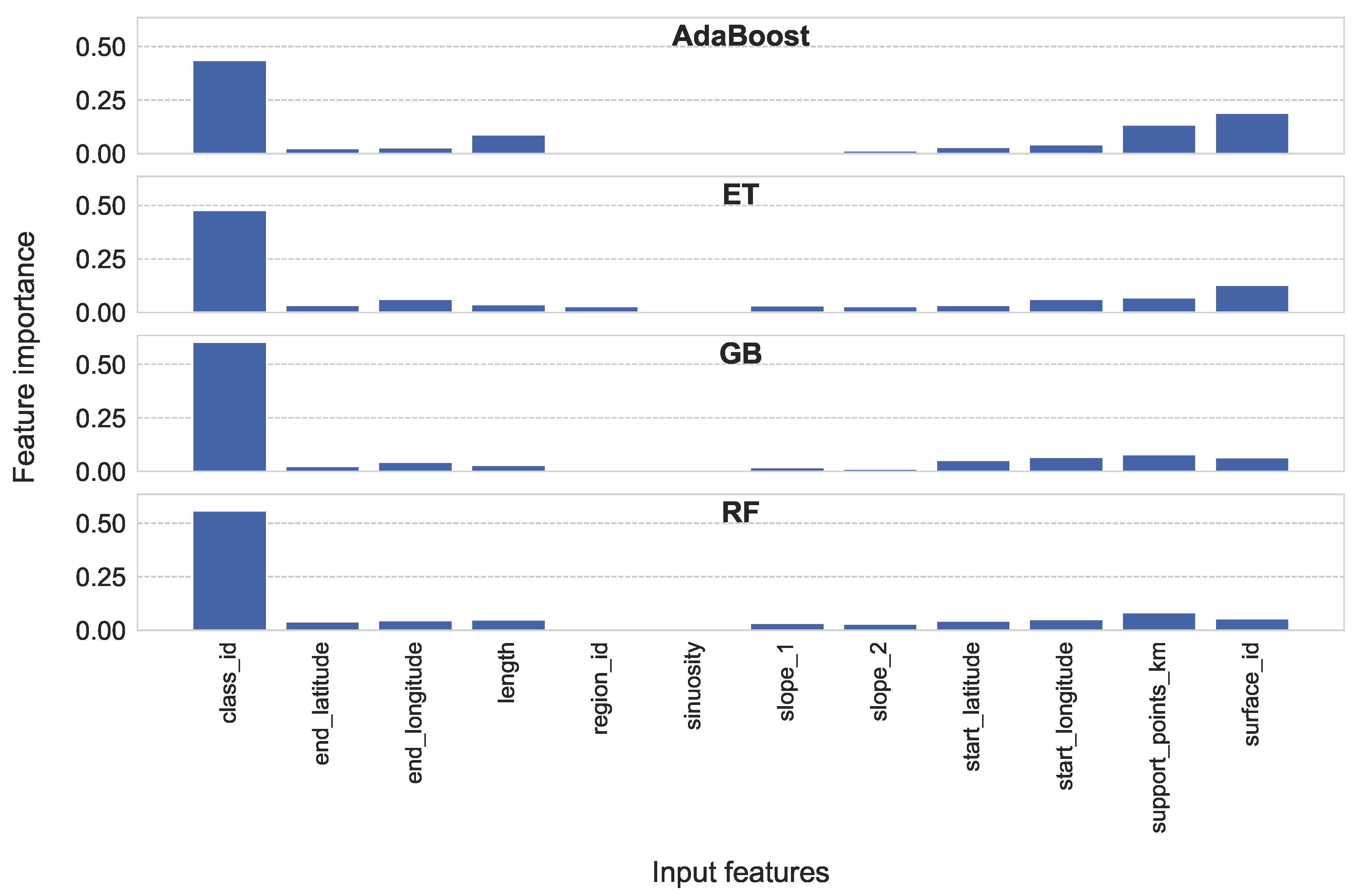
We show the feature importance distribution for the Basic input features in
Figure 7. The combination of Basic input features with the four SOM generated input features is given in
Figure 8 for the tree-based regression models, AdaBoost, ET, GB, and RF.
The most important feature for all DT regressors is the class_id. Additional features are rated differently by the four models. Concerning the four SOM generated features, these features are the second most important features for the four models when included.
4. Discussion
One main methodological objective is to investigate the potential of predicting average speed given only OSM road network input data. So far, little attention has been paid to usingg ML in the context of estimating average speed information, respectively, travel times, with OSM datasets. ML approaches can perform regressions without applying further (domain-)knowledge of the road segment that needs to be tagged with the average speed information. Generally, these approaches are data-driven without the need to engineer new features based on domain knowledge, such as, for example, the Fuzzy-FSE approach.
Our estimation framework is applied to three datasets covering two distinct regions in Chile and Australia and a wide range of average speed values per road class (see
Figure 2). We set up different combinations of input features: Basic, Basic + SOM, SOM, and PCA (see
Table 4). Therefore, we can evaluate and analyze the prediction results depending on the dataset and the applied input feature.
First, we discuss the performance and applicability of the estimation framework in
Section 4.1. Additionally, we summarize the essential findings concerning the different datasets and input feature modes. Second, estimation framework’s performance is compared with the Fuzzy-FSE on the BM and NNSW dataset from a general perspective (see
Section 4.2). Third, we consider the tree-based regressors’ feature importance and compare the important features with the input parameters of the Fuzzy-FSE with the input parameters of the the Fuzzy-FSE rules in
Section 4.3. Finally, we discuss constraints regarding the applicability of our ML-based estimation framework (see
Section 4.4).
4.1. Performance and Applicability of the Estimation Framework
When evaluating our estimation framework, we focus on its performance and applicability rather than on a regional analysis of the underlying datasets. In general, the regression results of the estimation framework indicate its applicability when predicting average speed based on the OSM road network. Our framework performs without systematic errors (see
Table 5 and
Table A3, and
Figure 5), although, for some ML models, the hyperparameter tuning could be slightly improved. This finding is emphasized by the random distribution of the average speed deviations for the combined dataset and the Basic input feature mode in
Figure 5.
Regarding the three datasets used for the ML models, the estimation framework improves its performance on the combined dataset due to the increase of datapoints. The ET model always provides the best regression results. ET generates its best result of the
score on the combined dataset with the Basic OSM road network input features, although the best RMSE score occurs on the BM dataset. This effect seems plausible since a larger amount of datapoints characterizes the combined dataset, but simultaneously, the data are more heterogeneous than the BM data (see
Figure 2). In the BM dataset, the range of the speed values (see
Figure 3) is smaller than in the NNSW dataset, which might be one reason for the better estimation performance of the framework on the BM dataset.
Concerning the different input feature modes, we find that the Basic mode with solely the OSM road network input features leads to the best overall regression performance. Using only the SOM generated input features or the two PCA input features, the regional datasets’ regression results are better with the PCA input features. However, on the combined dataset, the SOM generated input features are more valuable for the estimation framework due to the capability of the SOM to deal with heterogeneous datasets. This aspect is also recognizable when looking at
Table A3, where the SOM generated features alone embody enough information to enable the ET model to achieve
and RMSE
.
Figure 9 illustrates these results exemplary for the BM dataset. Herein, the generated
som_column and
som_row are colored according to two meaningful real-world characteristics, the road class and the average speed. After the training process of the unsupervised SOM is completed, the dominant road classes (
Figure 9, right) and the average speed values (
Figure 9, left) for every single SOM node are shown. Note that the applied SOM clusters the OSM road network input data in an unsupervised manner. We added the respective road class labels and the average speed information only to visualize the clusters. These different clusters are generated by similar classes or similar average speed values. Therefore, we gain information about similarities between the road classes or speed values. Besides, differences between datapoints of the same classes can be recognized. For both cases, the generated SOM structure resonates with the human intuition that the road class and the average speed are essential factors when classifying roads. However, we can recognize that some roads are clustered differently from other roads of the same type or speed profile. This finding shows that the interclass variance is relatively high and a massive task for any ML model to handle. The variance increases when looking at the same plots for the combined dataset (see
Figure 10). We find out that the more significant variance results in even more fissured regions in the 2D SOM’s output grid. Nevertheless, the overall structure still suits human intuition and is highly interpretable, which is one advantage of unsupervised SOM clustering.
Generating average speed reference data is time-consuming and costly, which often leads to sparse training data. Therefore, we investigate the ET regressor’s behavior on the combined dataset with the Basic input features by simulating missing labels in the training dataset by gradually reducing the number of training datapoints (see
Figure 6). The
scores decrease from above 80% to 78% while the missing labels increase from 0% to 60%. This finding indicates that we can use half of the training dataset’s labeled data on the combined dataset to predict the average speed with acceptable accuracy for two different regions. To generalize the investigation on the number of labeled datapoints, we need to generate additional datasets of different regions.
The average speed is predicted well for different regional datasets and a combined dataset by most regression models. This finding is documented based on the best regression results of
in the range of 76.38% to 80.43%. The ET regressor achieves RMSE scores between 1.89 km/h to 2.33 km/h lower than the RMSE of the Fuzzy-FSE. The excellent performance is a consequence of, among others, the selection of the appropriate ML models and the random split between training and test subsets (see
Figure 3). Since the average speed values are linked to specific road classes, we tend to be misled that each
class_id might contain values in close range to each other. Indeed, as shown in
Figure 2, the speed profile of the individual road classes’ speed profile varies largely, and the road classes of the different regional datasets are difficult to compare with each other. Concerning the variety of average speed values as a target variable, the ML-based estimation framework shows a first impression of its generalization capability. To fully evaluate and verify the potential generalization capability, the estimation framework has to be applied to additional datasets of different regions worldwide. Thus, the estimation framework predicts the average speed of road segments with OSM road network data. No additional data and domain knowledge is employed or needed. Furthermore, a more sophisticated tuning of hyperparameters could slightly improve the already good regression results.
4.2. Comparing the Performance of the Estimation Framework and the Fuzzy-FSE on the BM and NNSW Dataset
When comparing our estimation framework’s performance to the recently implemented Fuzzy-FSE, we find that the Fuzzy-FSE with domain knowledge performs better on the BM and NNSW dataset than our framework in the PCA and SOM modes of input features. Apart from this, the estimation framework outperforms the Fuzzy-FSE estimation on the BM and NNSW dataset with the Basic and Basic + SOM input feature mode. We further want to add that the Basic input features resemble the input data used for the Fuzzy-FSE.
Figure 11 exemplifies the speed deviation between the estimation error of the Fuzzy-FSE and the ET regressor with Basic input features on the BM and NNSW test subset. The individual errors are calculated as follows:
Fuzzy_error = Fuzzy-FSE prediction - reference speed values and
ET_error = ET prediction - reference speed values. The average speed deviation is defined as
Fuzzy_error - ET_error. This speed deviation allows the comparison of possible systematic errors from a regional perspective. As shown in
Figure 11, a random distribution of the deviations in the two regions occurs mainly in the NNSW region’s hinterland and the coastal area of the BM region. The deviation between the prediction errors is relatively small in the coastal region of NNWS and along the Ruta 5 in central BM. The inferior estimation performance of the Fuzzy-FSE becomes visible, especially in the central and western road segments of the test subset’s NNSW data. Again, the estimation framework’s better performance and the Fuzzy-FSE on the BM dataset is documented (see
Figure 11, upper map).
4.3. Analysis of the DT’s Feature Importance
The feature importance of the DT models enables us to investigate, to understand, and to link the OSM road network data with the average speed of road segments. We note that we analyze the feature importance primarily from a ML perspective. The shape of the feature importance plots (see
Figure 7 and
Figure 8) is relatively similar to a few standard features highlighted for each DT regressor. Regarding the feature importance of the DT models on the combined dataset with Basic as well as Basic + SOM input features, an important feature is the
class_id. This importance is identified as related to the average speed of a road segment and is similar to the valuable input parameters
road class of the Fuzzy-FSE. Besides, from a human understanding, the
class_id seems the best feature to sort average speed information. For the Basic input feature mode and the AdaBoost and ET model, the second important feature is the
surface_id. GB and RF list
support_points_km as the second important feature. However, their regression performance is weaker than the regression performance of the ET model. Again, the
surface_id is used as an input parameter to create the membership function in the Fuzzy-FSE. Hence, the tree-based regressors’ feature importance and the input parameters of the Fuzzy-FSE show some resemblance. From a human perspective, the importance of the
surface_id makes sense, since the surface of a road segment can vary even in the same road class.
When using the SOM generated input features for the regression task, all tree-based regressors, except for the RF regressor, rank the som_row_clustered feature as the second important feature following the class_id. This finding, combined with the regression result of , demonstrates that the SOM generated features embody enough information to enable the ET to a good regression performance. Generally, the other input features are more dispensable for the DT regressors.
4.4. Estimation Framework Constraints
Despite the strong performance of the estimation framework, few limitations exist and need to be discussed. As a first constraint, our framework relies on the dataset level on OSM road network data, which is freely available, and on GD-API reference data. The latter is not freely available.
Furthermore, we assume that the GD-API generates average speed values of road segments applicable as reference data but are also characterized by small discrepancies concerning the OSM road data. This matching discrepancy constitutes the second constraint. Since the ML models’ performance is affected by the accuracy and correctness of the reference data, the regression results of the selected regressor could be increased with a better match of OSM road network data and average speed values.
The third constraint is related to the principle distinction between rural and urban road networks. As mentioned before, our objective is solely the prediction of the average speed of rural road segments. The presented framework is not designed to predict the average speed in urban road networks. Since the estimation of average speed in urban regions depends on additional parameters such as traffic, our estimation framework needs to be adapted fundamentally to handle this regression task. For example, road segments shorter than 600 need to be included in the dataset. The main reason for this is that the urban road network consists mainly of such short roads. Besides, different input features, such as traffic data would be required.
As a fourth limitation, we point out that our estimation framework is designed as an initial step towards a generic, data-driven approach to estimate the average speed solely with OSM road network data. Our study demonstrated the ability of the proposed ML-based estimation framework to exemplary predict average speed for different, region-independent datasets. To verify the generalization, we need to modify and enhance the estimation framework and apply it to many more datasets. For example, some ML models do not handle the regional discrepancies in the BM and NNSW dataset well. These models could be replaced by more sophisticated ML approaches that can simultaneously cope with larger datasets.
5. Conclusions and Outlook
In this paper, we develop and evaluate an estimation framework for average speed in rural road networks based on a typical ML workflow and OSM road network data. This ML estimation framework is the first data-driven approach for predicting the average speed with only OSM road network data as input. The estimation framework is applied on road segments of three datasets covering different regions: the BM dataset, the NNSW dataset, and the combined dataset. We describe the datasets’ characteristics and the generation of average speed reference data based on Goggle Directions API. Two distinct unsupervised ML approaches, SOM and PCA, are included in the estimation framework to generate new input features. Especially, the SOM-based features offer a more in-depth insight into the data while also being capable of clustering the data in a meaningful way. A detailed evaluation of the regression performance with different modes of input features for each regression model is presented. We visualize the regression results of the best ML model for the two study regions. Besides, we compare the prediction performance of the ML-based estimation framework with the prediction performance of our recent Fuzzy-FSE, which is based on rules and domain-knowledge and the only available approach for this regression task.
As demonstrated, most of our selected ML models can handle the regression task on the different and heterogeneous datasets well. Thus, we can estimate average speed solely with OSM road network input features. In the context of predicting average speed, ML provides a data-driven alternative to the commonly applied approaches in routing applications such as fixed speed profiles and the rule-based Fuzzy-FSE, which relies on domain-knowledge. Furthermore, our framework’s estimation performance outperforms the performance of the Fuzzy-FSE on the two individual datasets and the combined dataset. We conclude that the ML model Extremely Randomized Trees (ET) is the most beneficial model regarding the underlying regression tasks. Additionally, the unsupervised SOM is capable of handling heterogeneous datasets to embody enough information in the generated input features to enable the ET model to achieve good regression results. Overall, the best performance of the estimation framework is achieved by the ET model on the combined dataset. One major advantage of our framework is the applicability to a diversity of road segments in terms of their road classes and their regional affiliation. However, the estimation framework is designed to predict the average speed of rural roads. Therefore, our framework needs to be adapted if it is applied to the estimation of the average speed of urban roads.
To conclude, this contribution is an initial step towards a generic approach to the estimate average speed of different road segments with OSM road network data as input. This finding is emphasized since road segments of two different regions in Chile and Australia are included in the study as exemplary datasets. The estimation framework can be used, for example, in routing engines when it is set up beforehand on data of the study area. Besides, it functions as a tool for the OSM road network data imputation to generate missing average speed values. Further studies and investigations in critical infrastructure could also benefit from a more accurate estimation of average speed values. Any modification of the fundamental methodological parts (see
Figure 1, data level to model level) would solely improve the already good estimation performance. However, further adjustments of the estimation framework and its implementation can be approached. For example, the ML models included in the estimation framework can be reduced to the most efficient models. Besides, a combination of a rule-based Fuzzy approach and decision trees, FuzzyDT, can be investigated to learn the Fuzzy rules during a training phase. Investigations can also focus on a more generic estimation of average speed based on our framework. These generalization abilities can be enabled when considering several road segments of many more regions worldwide. Including more data would foster the use and evaluation of deep learning models. For this purpose, some prerequisites are essential such as (a) reference data of further road segments covering additional regions, (b) enhancing our estimation framework for generalization, and (c) applying the framework to new OSM road network data to evaluate its generalization abilities.


