UrbanWater: Integrating EPANET 2 in a PostgreSQL/PostGIS-Based Geospatial Database Management System

Abstract

Incorporating data stored in a geographical information system (GIS) within the development of hydraulic simulation models is crucial for operating, updating, and hence redesigning water supply systems (WSS). Building and updating hydraulic models can be both time and resource consuming; moreover, the need to update infrastructure cadastral information makes the model itself outdated. In addition, typical dispersion of data across several databases requires extra effort to maintain the whole system and ensure it is properly assembled. Albeit there are some GIS-based hydraulic modelling solutions available, they typically use external connections to assemble all components resulting in additional costs and less flexibility. In order to be able to establish a single fully integrated data model towards global characterization of a WSS and associate hydraulic simulation, this paper proposes the specific implementation of an EPANET 2 model in PostgreSQL along with PostGIS extension. The system developed enables the construction of the model, hydraulic simulation, and storage of results within a single database. Required procedures and functions were coded either in pgSQL or Python and their execution were carried out using SQL statements. Finally, a case study was selected in order to test the system proposed. Results show that an integrated approach indeed allows the expedited creation of more realistic hydraulic models based on the stored cadastral information.

1. Introduction

1.1. Motivation

The design of management and operation methodologies for effective urban water supply systems (WSS) must take into consideration geographical information systems (GIS), which constitute an integrating platform of different sorts of information [1,2]. According to Shamsi [3], about 80% of the information potentially used by the water utility industry in operating a WSS is susceptible to being georeferenced. As such, a GIS approach may provide a WSS water utility with a set of opportunities, such as reduction in operational costs, reduction in response times, regularization of functional and/or structural failures, identification of investment priorities and establishment of contingency plans, amongst others.

The computational capacity increment of computers and the implementation of robust numerical methods for the determination of variables, such as flow and pressure, made hydraulic models a very much feasible and useful tool. However, its construction and update may well become resource consuming and a complex and long process—factors that impose a systematized use of such models principally among modellers of small dimension utilities.

Infrastructural cadastral information can be used in a GIS for the construction and maintenance of hydraulic simulation models. This avoids information redundancy and enhances model consistency. Georeferenced data characterizing physical components of a WSS (e.g., type of material, diameter, length and installation date of pipes, geolocation and operational state of valves), which can be stored in a GIS, constitute crucial components towards the construction of a hydraulic model. However, their continuous update turns a given hydraulic model into a misadjusted and consequently less accurate one. The link between GIS data and hydraulic models is of the upmost importance and ideally, a given hydraulic model should be dynamically readjusted in real time.

Some commercial solutions are currently available for WSS modelling provided with features that allow the establishment of links between GIS data, direct use of data, as well as data crossing. Nevertheless, those commercial solutions have been proven not to be totally effective as they are based on general approaches designed to cover a broad range of realities. In addition, in some instances, those commercial packages do not make modelling results immediately available to all sorts of users. Furthermore, some situations require specific procedures, for instance for the detection and correction of topological inconsistencies, or even for the evaluation of the overall completeness of the generated model. Typically, such procedures are not available in those software commercial packages. Finally, commercial solutions always have additional costs related to software maintenance and licensing. Most of the time, the solution comes with the development of an appropriate unique GIS-based approach that, working as a specialist assistant, enables a seamless integration of heterogeneous data sources and makes their comprehension within a single integrated platform simple [2].

Nevertheless, the integration of hydraulic models in GIS bears several challenges related to [4]: level of data accuracy and precision required; different perceptions about the role of both GIS and hydraulic models; effective and selective distribution capacity of the modelling result; update and maintenance of the model itself. In literature, there are currently a wide range of open source specialized tools available, which have proven to be robust enough for the purposes above, representing a low cost option for the end user. We believe that a combined use of such tools, along with appropriate adjustments, enables the construction of seamless integrated GIS-based hydraulic model platforms. Such an integrated platform is fundamental for simulation purposes as it allows the derivation of most uncertain variables and the anticipation of the impacts of different long-term perspective scenarios [5].

1.2. Aim and Objectives

In order to address some limitations pointed out above, this paper aims at developing a geospatial database capable of storing infrastructure cadastral data referring to the main WSS components, and also capable of storing data required for the dynamic characterization and generation of hydraulic simulation models. It was also sought that features of the system hereby proposed could be used in a wide range of desktop GIS applications. In the light of the main aim above, fundamental objectives were identified as follows:

• To design a conceptual model that enables the characterization of the different WSS components as well as the identification of information required for the hydraulic modelling process;
• To define topological and connectivity rules for each type of entity to be modelled;
• To develop functions and procedures enabling hydraulic simulation based on both graphic and alphanumeric data stored in the GIS.

In order to accomplish the objectives above, a PostgreSQL object-relational database management system (DBMS) was used along with PostGIS spatial extension—both are open source tools. As for the hydraulic simulation, this was accomplished by using the programming kit of EPANET 2 [6].

2. Background

2.1. The Role of GIS in Water Supply Management

The main purpose of a WSS is to provide users with potable water with enough quality and quantity, seeking to guarantee at the same time adequate operational conditions in the event of emergency situations, such as urban fires. A typical WSS infrastructure consists of pipes, pumps, tanks, valves, flowmeters, air valves and other hydraulic components

From the management perspective of entities, relevance of GIS technology in WSS management becomes evident if one takes into consideration the nature of information continuously produced by such systems, the spatial distribution of their components and the spatial localization of consumers and demands [7,8,9]. According to USEPA [10], the nature of WSS information is principally geospatial; as such, its management involves the use, manipulation, and analysis of georeferenced data [11]. These may well refer to the localization of a consuming point, pipe crack, or may refer to the localization of sensitive consumers (e.g., hospitals, schools, restaurants, etc.). Development and maintenance of a well-organized and up-to-date infrastructural cadastre is time consuming and cumbersome [12], but constitutes a fundamental instrument to support efficient and effective decision making, to reduce operational costs, to reduce response times, to define investment priorities, to establish contingency plans, among others.

At a global scale, the evolution of GIS in the sanitation sector took place in the late 1980s of the 20th century. In the following decade, the use of GIS technology for infrastructure management or maintenance operations became much more common. Towards the end of the 1990s, the emerging commercial software packages with far friendlier interfaces made GIS a broader interdisciplinary technology, currently being used in a wide range of fields, such as hydraulic modelling and water quality evaluation [13], cited by [3].

According to Shamsi [3], GIS solutions have been mainly adopted towards mapping, monitoring, modelling and maintenance purposes of WSS. This is mainly due to the capabilities of GIS to characterize the whole system, to identify critical spots and to delineate alternative scenarios, and to schedule and register interventions (e.g., record of event, size, status, type of material, type of soil). GIS geoprocessing capabilities, such as overlapping and manipulation of different layers of information, enable more expeditious and effective geospatial analysis and planning operations. Topology is certainly a central defining feature of a GIS [14] and hence the consideration of topological properties in digital representation of a WSS guarantees connectivity between its components, enabling the generation and development of a topologically correct global hydraulic model—this is indeed one of the main focuses of this paper.

Finally, GIS may be seen as an integrating platform of information technologies. Such characteristic along with mobile communication of data capabilities allow the search and production in real time of georeferenced information, eventually enabling the usage of decision support tools. Altogether, the technological characteristics stated above may potentiate hydraulic modelling if implemented within a GIS environment.

2.2. Hydraulic Modelling and Its Integration into a GIS

The ability of determining computational flow and pressure in a given WSS has been always of great interest among the management of entities. This is crucial mainly for the planning, conception, and operational purposes of WSS capable to serve consumers efficiently and securely. In order to determine the variables above, different methods have been proposed so far, such as graphical methods, physical analogies, and mathematical modelling [15,16,17].

The emergence of personal computers in the 1980s of the 20th century, made mainframes redundant and hydraulic modelling became available to a broader range of target users. In addition, the possibility of modelling water quality as well as more complex WSS components (e.g., pumps, pressure relief valves), and also the possibility of using graphical interfaces in computational applications, largely prompted the usage of the hydraulic modelling approach by management entities [16]. In addition to water supply management, hydraulic modelling is an important tool for asset management activities, operational control plans for monitoring and improving water quality [1], definition of district metered area [18,19], establishment of water leaks programs [20,21,22,23], and failure risk analysis [24,25,26].

Typically, the construction of a WSS hydraulic model requires data and information spread across several different information systems, which may well turn into a complex and time-consuming process. Data required for the purpose strongly depend on the components considered in the WSS and on how their behavior is actually modelled. Overall, required data are related to [10] physical characteristics of the network components, water consumption data, height data, and operation rules. All data above can be stored and managed within a single platform—GIS.

Historically, the conception and implementation of hydraulic modelling in a GIS platform was prompted by users’ curiosity and expectations. Geographic representation accuracy and associate alphanumeric data accuracy and precision have been always privileged in GIS. In addition, connectivity representation (very much supported by GIS) is fundamental to hydraulic modelling. Moreover, computational capabilities, availability, sophistication and interoperability of several geographic information management applications provided GIS with the required maturity for its usage both as front-end and back-end in the context of hydraulic modelling.

The integration of these avenues, GIS and hydraulic modelling can be defined as the process in which insertion, deletion, or update operations of data stored in the system are reflected on the hydraulic model; in turn, results of the modelling process are managed and stored in the system too. Shamsi [27] established a three-level classification of hydraulic modelling: interchange, both systems are operated separately, information of interest is exchanged by a an intermediate file; interface, both systems are operated separately too, there is no need though for an information exchange file, a link is established between two systems based on protocols and compatibility structures; true integration, corresponds to the most sophisticated level of integration in which both systems operate as a single unit.

2.3. Topology and Connectivity Rules

When constructing the hydraulic model based on data stored in the geographic database, assuring connectivity between WSS components is fundamental for a consistent functional relation between those components. Defining and implementing topological rules can achieve this. Topology is indeed crucial to avoid connectivity errors and aims to represent how pipes, valves, and other accessories are connected in reality to form a single network. In order to explicitly represent and store spatial relationships and their properties, data topological frameworks are commonly used [14]. The topological representation of a geometric network that is behind a WSS may be accomplished by considering an abstraction based on the logic model of a graph, i.e., a network of nodes and edges.

For point features (e.g., valve, flow meter), the following rules should be established [28]: they must be located at the end of the graph’s edge and must intersect one of the points of a linear element’s boundary (e.g., pipe); an entity located at the end of a section must be of a single type and entity duplication is forbidden. Typical errors may consist of, for instance (see Figure 1), orphan nodes, snapping errors (such as under or overshoots), duplicate entities, non-segmentation of linear entities at the intersection point of its interior with the point.

For linear features (e.g., pipe), the following rules must be observed: such entities cannot self-overlap or self-intersect; overlapping linear entities can be allowed if these run in reality in parallel; each edge’s end must intersect a graph node; overlapping errors may be due to accidental digitalization of same spatial entity, or due to existing similar geometries associated with 2D nature of geospatial information; snapping errors may occur between an edge’s end and a WSS entity modelled by a node, or may also occur when the node is accidentally missing (see Figure 1).

Complementarily to general topological rules, it is recommended that the establishment of other rules reflect specific functional and connectivity characteristics of different entities and their interactions in real world cases. Such rules may be used to model situations such as two pipes with different diameter need a reduction cone, a T junction needs to be connected to three pipes.

3. Methodology

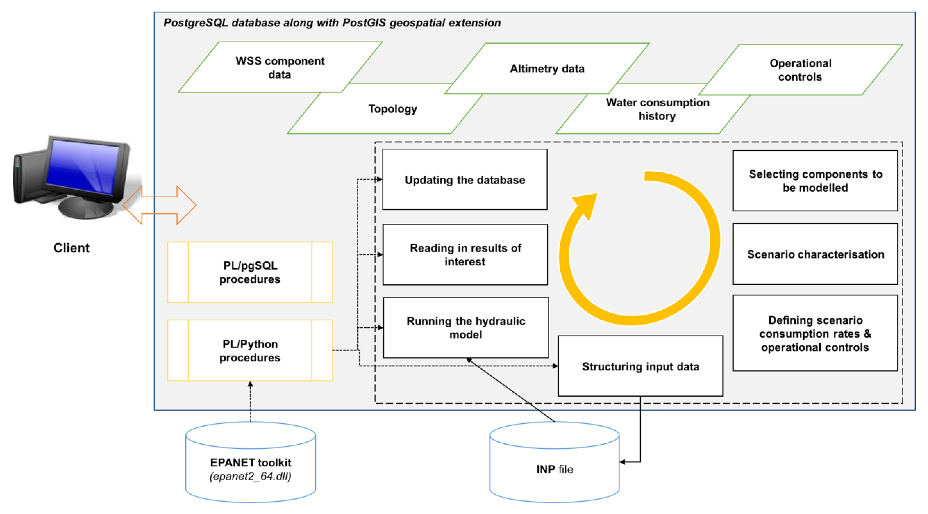
3.1. General Characteristics of the System Proposed

The system proposed in this paper is based on a client/provider approach in such a way that implemented functionalities are independent from the front-end used. As explained above, conceptual model development was based on the logical model supported by graph theory, and associate physical model was implemented in PostgreSQL 9.3 environment, along with PostGIS 2.1 spatial extension, enabling spatial object management. Spatial entities and associate relationships considered allow the characterization and management of infrastructure cadastral information; in turn, such information enables generation on the fly of hydraulic models based on EPANET 2 [6]. Several scenarios may be simulated, and respective results stored in the geospatial DBMS. These can be either displayed through mapping or accessed via tabular form (Figure 2).

Given the capabilities of the geospatial DBMS, several functions and procedures were developed in order to automatically populate attributes of interest, to validate connectivity rules, to update topological relationships, or to run hydraulic simulations. Such functions were in turn associated with other trigger procedures that prompt and run them every time a certain operation occurs (e.g., any insertion/deletion of spatial entities, or any other WSS update). These were all coded either in pgSQL or Python.

In order to run a specific hydraulic simulation, SQL instructions must be executed using the functions and procedures above plus respective input data, such as hydraulic options, time windows, water consumption values, topological information and heights, or physical characterization of geometric network components. The associated hydraulic model is then either generated from scratch or simply updated based on the data above, and the needed WSS code is specified.

3.2. Data Model

In the data model, main WSS entities are defined and their geospatial relationships are established in order to model real world ontologies and their interactions. As such, entities that enable physical characterization of the WSS, storage of geometric network topology as well as water consumption records for each connection are defined. For illustration purposes, Figure 3 depicts (just for the case of valves) attributes and domains considered to characterize a given scenario to be modelled and to specify temporal options, along with relations established to associate results with modelled components and with the respective scenario.

Table 1. Data model: main water supply system (WSS) geospatial components considered.

WSS Component	DB Table	GIS Geometry	Hydraulic Model
Fire hydrant	boca_incendio	Point/Polyline	✗
Borehole	captacao_subterranea	Point	Node
Pipe	conduta	Polyline	Arc
Water meter	contador	Point	Arc
Discharge	descarga	Point	✗
Pump	eletrobomba	Point	Arc
Tank inlet	entrada_reservatorio	Polyline	Arc
Hydraulic accessory (e.g., coupling, fitting, reducer)	equipamento_hidraulico	Point	✗
Fire hydrant	marco_incendio	Point	✗
Localised consumption	ponto_entrega_alta	Point	Node
Service line/Connection	ramal	Point/Polyline	✗
Tank	reservatorio	Polygon	Node
Control valve (e.g., pressure reducer)	valvula_controlo	Point	Arc
Check valve	valvula_retencao	Point	Arc
Valve	valvula_seccionamento	Point	Arc
Air valve	ventosa	Point/Polyline	✗

summarizes those WSS components considered, the associate relational table (as defined in [29,30]), the respective geometry used to represent them in a GIS platform, and which graph element is used to model them.

Database tabular attributes, associate domains, and default values were defined for each WSS entity. Given the existence of the same type of table fields for distinct entities and the need to implement mechanisms to validate domain values, domain masks were defined (e.g., operational state, conservation state, diameter of different components, among others).

In order to guarantee referential integrity between entities, database foreign keys were defined accordingly. In addition, in order to access data more efficiently, different GiST indices were established for database primary keys as well as for geometric attributes.

Required entities and respective spatial relationships for the modelling process enable the establishment of general options, the characterization of water consumption rates at graph node level, and the establishment of an operational control related to each simulated scenario. Database tables are also included in order to store WSS component attribute data and also simulation results (irrespective of static or dynamic simulation).

As an illustrative example, let us consider opcoes and cenario relational tables. These relations allow the completion of the characterization of each hydraulic simulation scenario. Each tuple of cenario relation allows the establishment of the simulation ID code, the code of the system to be modelled, the consumption units, continuous head loss equation, and the set of temporal options. The attribute referring to temporal options consists of a foreign key that refers to the primary key in op_tempo relational table (Figure 3 above) enabling the sharing of the set of temporal options tuple, and in turn establishes the entire simulation time window, hydraulic time step, pattern time step, report time step and other similar options.

Establishing two relational tables carries out the result storage referring to each modelling scenario. Such procedure is associated with each modelled component (Table 1 above). For each component, the relation whose prefix is inp_<nome componente> is bound to include data independent from the computation time of that component; in turn, hydraulic simulation results are included in the relation whose prefix is inp_rpt_<nome componente>.

For hydraulic model components represented by graph nodes, the attributes that were generically considered were consumption rate, head, and pressure. In turn, the attributes that were generically considered for graph edge entities were velocity, flow and head loss. Due to the fact that some WSS entities are modelled in GIS and in the hydraulic model differently (e.g., a valve is hydraulically modelled as an edge, and as a node in GIS), not only respective results were associated with those entities but also their upstream and downstream nodes. This way, when the hydraulic simulation is carried out, it is possible to directly manage those entities through their associate GIS geometry by searching and accessing their attributes and simulation results at once.

Considering WSS entities specified in a given scenario, calibration_param relational table enables the definition of new values distinct from those theoretically established beforehand for each hydraulic parameter. (e.g., roughness coefficient). The mentioned tuples aim at calibrating the hydraulic model.

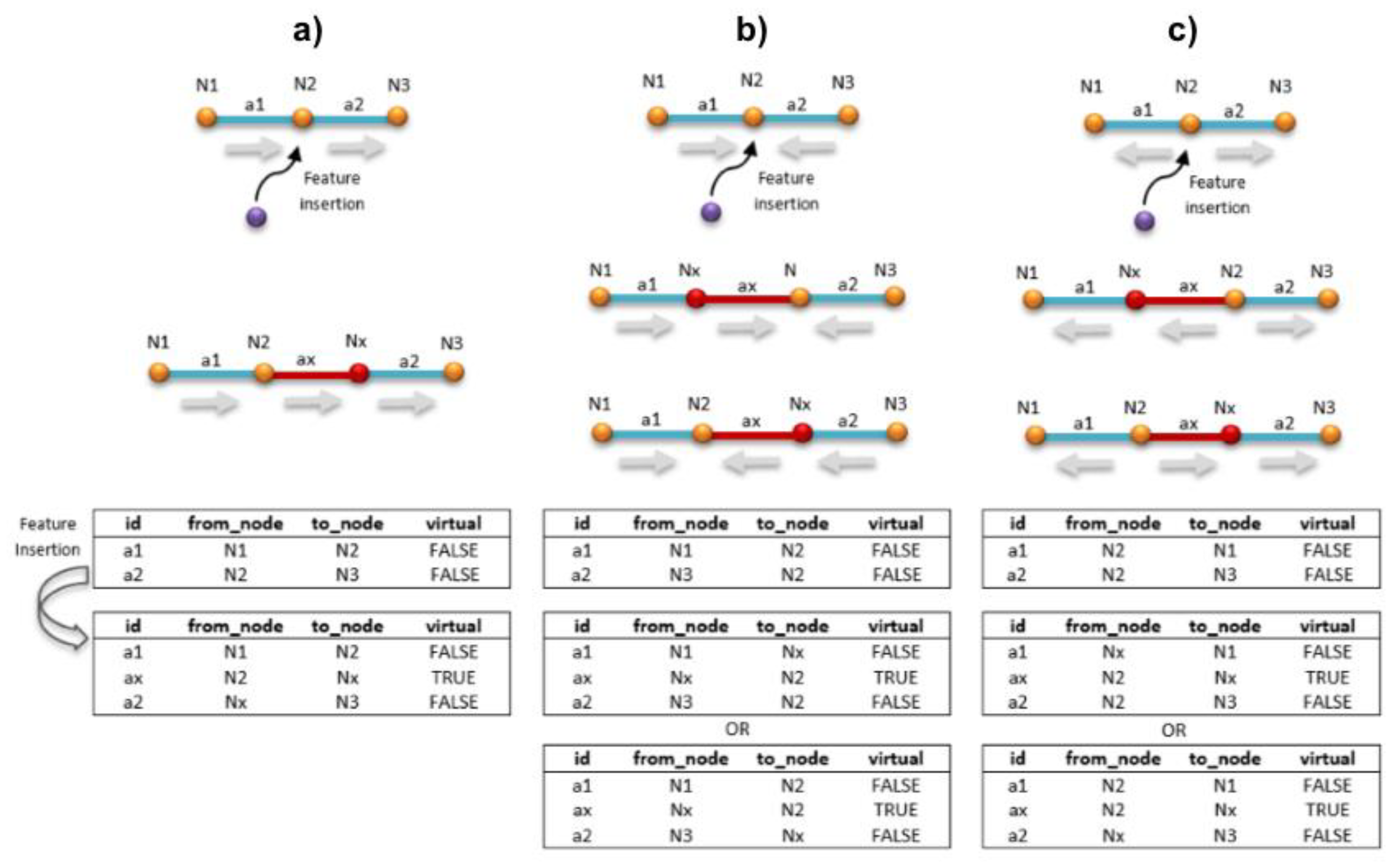
3.3. Topology: Connectivity Rules

The connectivity rules mentioned in Section 2.3 aim, for instance, to establish the maximum number of entities that a given entity can intersect to, to avoid the fact that more than one entity is located at a given node (e.g., a meter or a valve), to evaluate whether one or more vertices of a linear entity’s border (typically, a valve) can be removed or not or to evaluate the compatibility between geospatial information and the hydraulic model, among others. A set of 37 connectivity rules were implemented through different trigger procedures summarized in

Table 2. Trigger procedures referring to WSS components and meant to maintain the arc-node topological model as well as the case they are based on (which is function of the direction of adjacent pipes).

WSS Component	Trigger	Associate Trigger Procedure	Case
Pipe	inp_no_arco_ins inp_no_arco_upd inp_no_arco_del	inp_no_arco_ins inp_no_arco_upd inp_no_arco_del	-
Water meter	inp_no_arco	inp_no_arco_elementos_orientados	I
Control valve
Check valve
Pump	inp_no_arco	inp_no_arco_eletrobomba	I
Valve	inp_no_arco	inp_no_arco_valvulaseccionamento	II ou III

.

Trigger procedures designed and coded in PL/pgSQL are meant to undertake the validation of connectivity rules. For each relational table, a trigger procedure was implemented, prompting associate procedures and functions. Rules are checked for each tuple, taking into account the type of SQL operation involved (insert, update or delete), if a given rule is not matched, an exception is registered. Exceptions terminate transactions involved and associate updates are not accomplished. To illustrate this, algorithm 1 shows pipeConectivityRulesInsert() trigger procedure, this aims at validating respective connectivity rules for each tuple when their insertion into pipe relation occurs.

Algorithm 1. Pseudo code of the algorithm implemented to validate connectivity rules after a new pipe is inserted into the system.

Procedure pipeConectivityRulesInsert(): If IsSimple(NEW.geom)==TRUE And IsClosed(NEW.geom)==False    ptF = st_startpoint(NEW.geom)    ptT = st_endpoint(NEW.geom)    For each type of WSS component       Count number of intersected features by ptF       If Count > 0          Call Verify connectivity rules for intersected feature          If rules not verified             Raise Exception          End If       End If      Count number of intersected components by ptT       If Count > 0          Call Verify connectivity rules for intersected feature          If rules not verified             Raise Exception          End If       End If    End For each    Count pipes touched by ptF    Count pipes touched by ptT    If Count ptF>3 or Count ptT>3       Raise Exception    End If Return New Else    Raise Exception End If

Once the connectivity rule validation is carried out, entity representation in the geometric network is updated based on graph arc-node topology. The implementation of this is based on the premise that any infrastructural cadastral update leads to a global geometric network update too. Topological information maintenance was implemented in a coherent way so that computational time is reduced when the associate hydraulic model is generated.

As mentioned in the previous section, the geometric representation in GIS of some WSS components may differ from that in the hydraulic model (Table 1). As such, the consideration of mechanisms to update topological information in order to make both abstractions compatible were needed. As an example, entities such as control valve and pump, among others, are modelled as an additional arc in between two adjacent arcs corresponding to the two bits resulting from the pipeline split, due to topological consistency, an additional node is also required (Figure 4).

Given that certain WSS entities constitute one-way water flow components, associate trigger procedures reflect this characteristic, whose implementation is based on the respective GIS layer as well as entities’ alphanumeric attributes (e.g., type of pump). In cases like this, any topological information update is accomplished by running inp_arc_node “after trigger”, which is specified for each modelled relation and associate trigger procedure.

3.4. Representing WSS Components in the Hydraulic Model

For each WSS component, a corresponding representation in the hydraulic model was established according to their specific characteristics and hydraulic performance (see

Table 3. Entity(ies) considered to represent the WSS components within the hydraulic model.

WSS Component	Corresponding Entity(ies) in the Hydraulic Model
groundwater reservoir	Reservoir
pipe	Pipe
water meter	EPANET manual gpv General purpose valve (GPV) with a characteristic head loss curve
pump	Pump
tank inlet	Pressure sustaining valve followed by a check valve
localised consumption	Reservoir with fixed water level and pipe with unitary length
tank	Tank with variable water level linked to the network by a unitary pipe per water exit
control valve	Control valve
check valve	Check valve
valve	General purpose valve

).

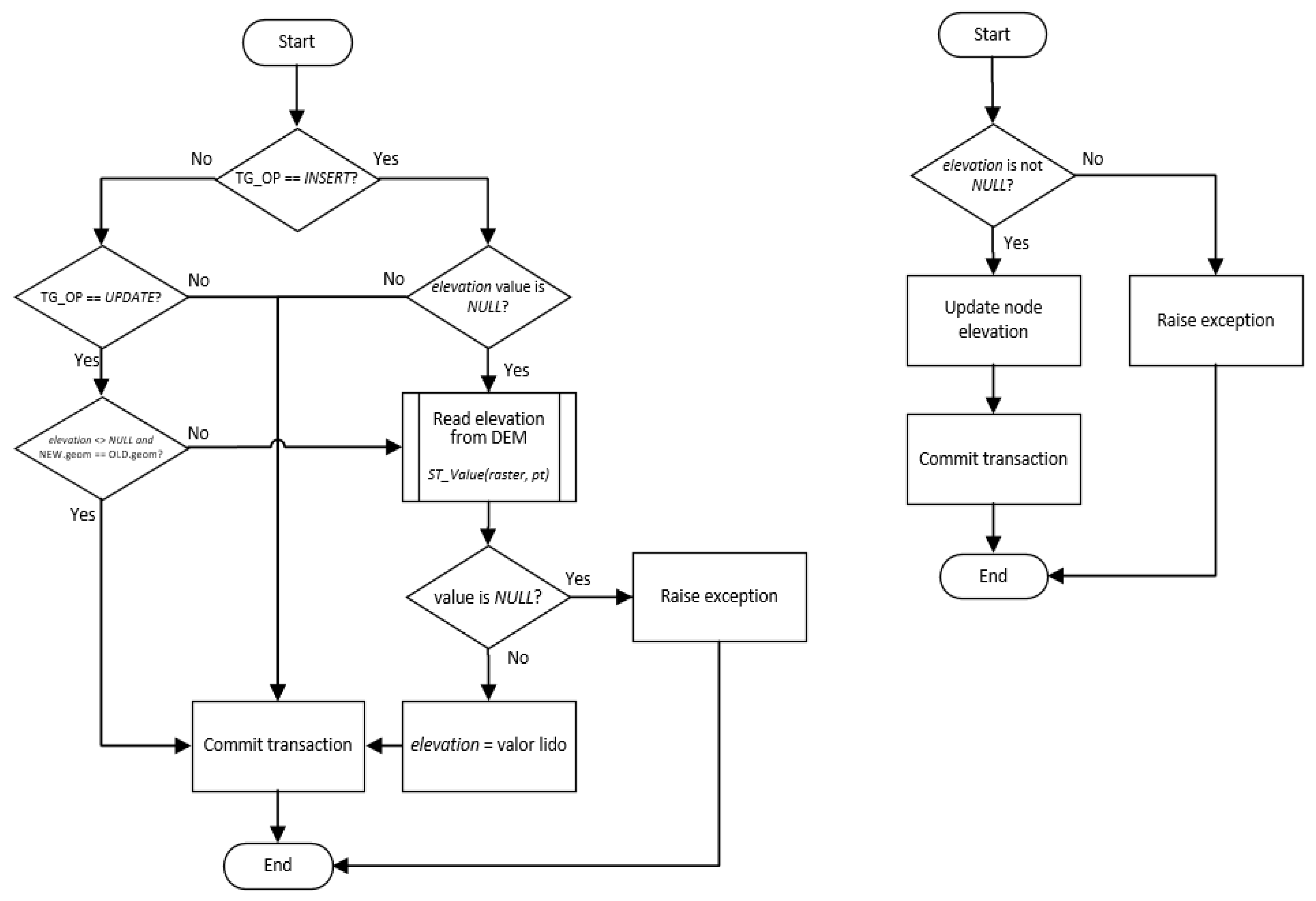
3.5. Height/Elevation Information

Including the Elevation attribute for all WSS components of point geometric type carried out the consideration of height information. In turn, as far as pipelines are concerned, such information was associated with their junction nodes.

Two different situations and respective methodologies may be identified beforehand. When an Elevation’s value is missing, it is retrieved by intersecting the associate WSS component with a raster format digital terrain model (DTM). This is accomplished by the elevation_insert trigger procedure (see Figure 5), which was implemented according to PostGIS functionalities in terms of raster data access and storage. By defining the elevation trigger procedure in the relevant relational tables, this is evoked by each tuple and by instructions of insert or update types. Another situation refers to height data update of a given junction node. This is accomplished based on a WSS component inserted at the same location and whose altitude value is not missing (elevation_updt trigger procedure, see Figure 5). In this case, node_elevation trigger was defined for each relational table coupling it with the respective trigger procedure.

3.6. Consumption Data

Water consumption data along with volume of water losses are meant to characterize the overall demand upon a WSS, both geospatial as well as temporal. The information above is indeed of major importance for the definition of the associate hydraulic modelling scenario. This is accomplished in practical terms by associating the different consumption figures, which occur along a pipeline section, with their respective nodes. In our system, the required relational tables for base consumption rate specification were defined for each node of a given scenario; in addition, in case of long-term simulations, specific relations were also implemented for the establishment of temporal patterns (see Figure 6).

The implementation approach adopted enables the specification for each node of a set of tuples representing consumption rates, cumulative among them, which may well have distinct patterns. Each pattern is characterized by a set of multiplicative factors that are defined in the Pattern_points relational table. This approach enables the structuring of information in such a way that it is easily accessible and can be inserted into INP file (see Section 3.8). INP file is responsible for prompting the static/dynamic hydraulic simulation run.

Water consumption characterization may be accomplished automatically based on a simplification of consumption rates consisting of the concentration of rates at the from-node and/or to-node of the corresponding pipeline section. junction_of_demand procedure (coded in PL/pgSQL) considers the intersection relation between the branch’s border and the pipeline section’s interior. This way, for each branch, the distance between its intersection point and the pipeline section from the node is calculated—the water consumption rate referring to that branch is then associated with the closest node (a junction node of the pipeline section). Such procedure is supported by st_line_locate_point function, in PostGIS spatial extension. In order to compute the consumption rate for each consumption, associate water meters, and their invoicing records are taken into account, which is characterized in the geospatial DBMS through the customer relationship management system (CRM).

Given a particular hydraulic scenario, the base consumption is computed then for each node and inserted into the Demand relational table. For the purpose, assign_demand procedure was developed based upon the procedure described above whose input parameters are as follows: the hydraulic scenario code, percentage of head losses in the system, total number of invoicing years taken into account for the average consumption evaluation, and also (in case of a dynamic hydraulic simulation) the consumption diagram—in cases where the consumption diagram is not available, consumption rates are computed then based on the amount of served population within the modelled geographic area.

3.7. Operational Controls

In order to reflect the WSS operating conditions in the hydraulic model (e.g., start and stop of a pump governed by a tank water level), operational_controls procedure was considered to enable the definition of simple controls (controls) or multiple condition controls (rules). Each tuple corresponds to a specific control, which is classified according to its type and is associated with a specific scenario as required by EPANET toolkit syntax. This is checked by validate_operational_control procedure coded in PL/Python.

3.8. Creating the Hydraulic Model and Running the Simulation—The INP File

After defining all entities and their attributes responsible for the management of the WSS, physical characterization information, height information, topological information, water consumption information, and operational controls, as well as hydraulic and temporal options for the given modelling scenario, it is possible to fill in all INP file sections. The INP file is generated by the cria_inp procedure (coded in PL/Python), whose input parameters are the hydraulic scenario code, and the geographic area code. SQL instructions to be carried out consist fundamentally of common selection procedures or through table joins, by selecting table fields present in different tables (projection) according to relevant information for purposes of section characterization. Data access is accomplished using plpy module, which is automatically imported when PL/Python is used in the DBMS. Each record is then written in the output file following the syntax rules of each section [31].

PostGIS functions are equally considered for the retrieval of relevant information. In characterizing [JUNCTIONS] section, both st_x and st_y functions enable the retrieval of (x,y) coordinate pair from the type of point geometry that characterizes each junction node.

PL/Python processa_inp procedure was implemented for the purpose of running the hydraulic modelling, either static or dynamic (see Figure 7). The procedure above is prompted by the INP file created beforehand and associate results are inserted thereafter in the database for each modelled component, this is carried out according to the temporal pace considered in the scenario in hand. For each component, (inp_<entity_name>) relational table is considered where data are independent from its initial state and from the computing period of time (e.g., diameter, length, altitude), (inp_rpt_<entity_name>) relational table is also considered aiming at storing corresponding results.

The hydraulic modelling is actually accomplished using the set of functions as follows, ENopenH – ENinitH – ENrunH – ENnextH – ENcloseH, also referring to ENgetxxx functions in order to access interim results of each computing stage (Figure 7). LoadLibrary method, of windll (ctypes module) class, enables the loading functions above through the EPANET toolkit.

4. Case Study: Casal-do-Ribeiro WSS

4.1. Using UrbanWater Plug-in

A hydraulic simulation, either static or dynamic, is achieved by running procedures described in Section 3 through appropriate SQL instruction sequences. For this purpose, the UrbanWater application was developed—a plug-in implemented in Python for Quantum GIS (QGIS) platform (Figure 8).

UrbanWater plug-in enables the specification of required parameters. It also enables the filtering of results stored in the database related to the respective simulation scenario. In addition, for node or edge-based feature class layers, it is possible to select which parameter the user wants to be mapped, in such case, associate display properties and legend are automatically updated accordingly. The interaction with PostSQL DBMS is undertaken through psycopg 2.5 adaptor for Python programming language.

In addition to enabling the generation of thematic maps based on the selected parameters, UrbanWater also has a feature that enables graph plots of results obtained for the different selected parameters in an active GIS layer (whose Python code implementation makes use of matplotlib library). For features represented in the hydraulic model by nodes, consumption rates, head, and pressure are presented; in turn, for edge-based features, the velocity, flow, and continuous head loss are shown along with results obtained for both upstream and downstream nodes.

4.2. Case Study Description

Casal-do-Ribeiro is a rural civil parish located in Ourém district (Leiria province, west-center of Portugal’s mainland). The WSS has its origin in a groundwater source (SL1) and the water is raised up to the main local reservoir through a submersible pump. The treated water is later distributed and gravitationally added up to Casal-da-Fonte pumping station. The adduction has an extension of 1.8 km, consisting mainly of PVC and HDPE materials. The distribution network has a total length of 39.1 km, consisting of PVC pipes (99.8%), where 50% of the diameters are less than or equal to 110 mm, the maximum diameter is 160 mm, with 846 customers, and 817 connections. Cadastre of the different WSS in Ourém district is stored in computer aided design (CAD) format (the geometric component) and the corresponding alphanumeric data are stored in Oracle 8i DBMS. A module implemented in Bentley MicroStation enables management and synchronization of information stored across both data sources. For our purposes, vector and alphanumeric data were joined and later exported to ESRI shapefile format for each entity of interest.

In order to facilitate data manipulation for each component, the data above were uploaded onto a PostgreSQL DBMS. Using SQL statements, domains and attributes of the different entities were adapted in terms of the proposed data model, as well as the validation and solving of conflicts resulting from non-compliance with connectivity rules and topological errors. The characterization of customer consumption related to each installation was obtained from the invoicing system based on 2012–2013 average daily consumption.

Given the fact that some implemented features require height data for each junction node, a digital terrain model (DTM) was generated and stored in raster format.

The associate modelling scenario was defined by considering all physical components that make up Casal-do-Ribeiro WSS, according to the existing cadastral information and the proposed data model. In order to take into account the largest volume of information possible (e.g., consumption rate patterns), a dynamic simulation approach was considered, which corresponded to a 72 hour duration time.

Operational controls related to the pumping equipment operation, derived from the implemented remote management system, were considered. Control valve parameters were established according to the maintenance records.

4.3. Running the Hydraulic Model

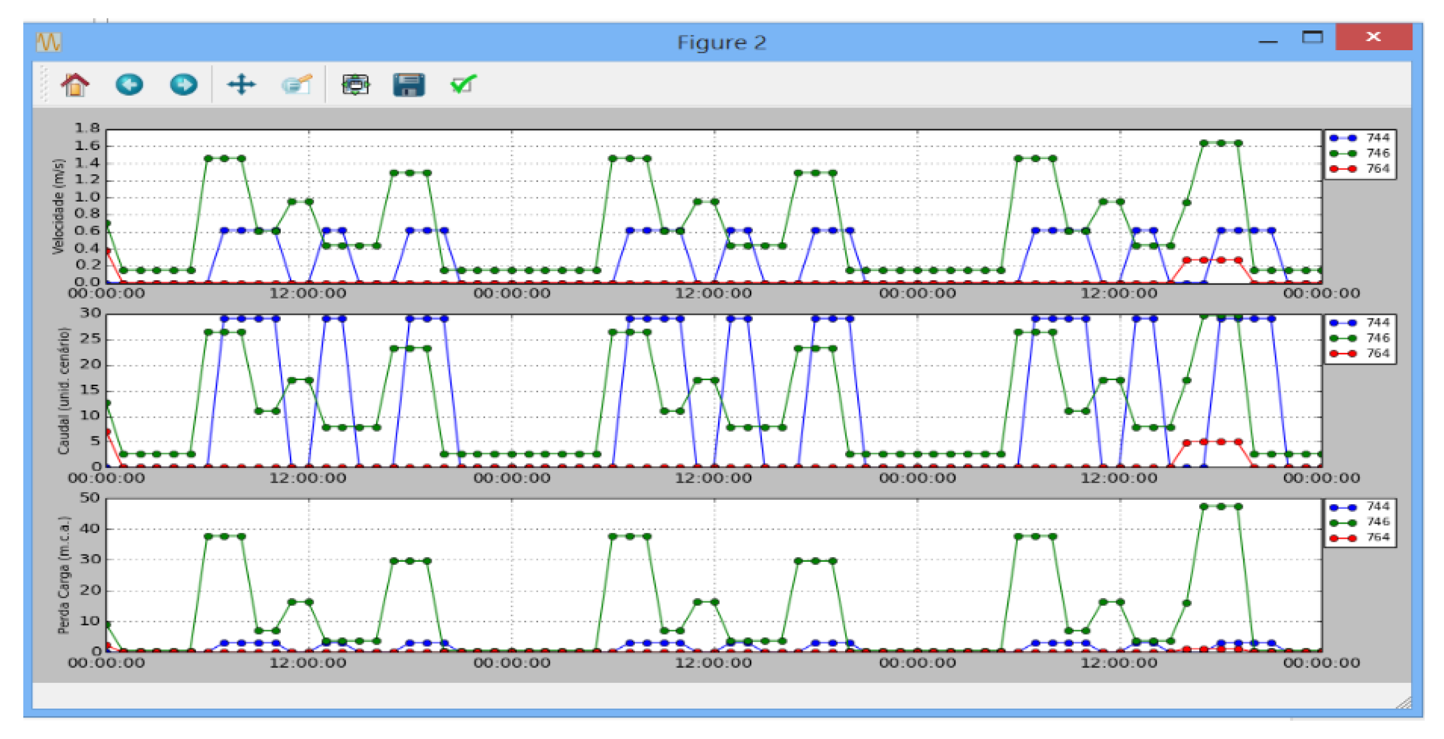
As explained above, creating the INP file, running the model, and processing the results are accomplished by defining and executing a series of different SQL statements. Firstly, a set of temporal options was defined by inserting the respective tuple into op_tempo (schema modelacao) relation. Then, the scenario was defined through create_cenario procedure, alternatively, the tuple can be inserted into cenario relation, also indicating the WSS component selection criterion. Each node may have different consumption categories, each one having, in turn, its own consumption diagram. The INP file was then created, the resulting hydraulic model was analyzed, and results were read and inserted into the database. For purposes above, SQL statements below were executed as follows:

SELECT modelacao.cria_inp(’CRB-MED-72H’);

SELECT modelacao.processa_inp(’CRB-MED-72H’);

The first SQL statement above accomplishes the generation of the INP file, referring to the modelled scenario, which is the input for EPANET model (Figure 9).

The second SQL instruction above performs the hydraulic analysis using functions of the EPANET toolkit.

4.4. Results

Figure 10 depicts graphic results obtained for the selected system component: velocity, flow and head loss. Visual representation of graphic-based results is enabled by associate features implemented in UrbanWater plugin (QGIS).

Based on the scenario previously setup, analysis of velocity was carried out for pipe sections (Figure 11). A filter was applied to data to be mapped through the plugin developed, selecting both scenario and simulation time window wanted.

In addition to the quick generation of the INP file, another advantage of storing results in a geospatial DBMS is the possibility of a joint usage of both DBMS and mapping functionalities. Figure 12 exemplifies how the plugin’s database (DB) manager was used in a SQL query to geospatially map all pipes in which velocity is higher than the maximum threshold allowed.

5. Conclusions

5.1. Final Considerations

Establishing the conceptual model took into consideration the definition of required entities that enabled an EPANET 2 based hydraulic modelling. The approach undertaken did not simply replicate standard EPANET entities; in fact, we also sought WSS cadastral data management totally based on an open source DBMS, upon which different hydraulic scenario modelling capabilities and associate analysis procedures were implemented. Procedures and functions implemented within the DBMS in imperative programming languages enabled the representation of a given WSS that is totally compatible with the hydraulic numerical model defined within the INP file. This fact allows the assembling of WSS cadastral data as well as both input and output data from the hydraulic modelling simulated scenarios, within a single database. In addition to this characteristic, the generation of the INP file, for the analysis and processing of results obtained, further enables, in a complementary way, their usage in dedicated applications, requiring for instance specific analysis procedures not available in the standard EPANET toolkit.

The system solution proposed in this paper implements the most common EPANET options in such a way that it considerably reduces the amount of effort, resources, and time typically spent to build adequate hydraulic models. This fact is indeed achieved by eliminating common manual tasks of converting and establishing the correspondence between input data and the hydraulic model, or even, making them compatible. Results obtained for the different scenarios simulated can be used to produce reports and/or indicators. Managing and accessing results obtained are clearly potentiated by standard DBMS features, such as queries, multiuser access, or web mapping services.

As a final remark, integrating the capacity of the WSS conversion into a hydraulic model, running the hydraulic simulation, and making results available through a geospatial DBMS, allows one to perform a series of different kinds of analyses that all together makes the system developed an added value for evaluation and optimization purposes of WSS management.

5.2. Future Work

As far as established connectivity rules are concerned, it should be stressed that those rules impose beforehand rigid editing/digitizing procedures on WSS cadastral data. In order to overcome situations of simultaneous feature editing, the insertion or update order of any alteration should consider each connectivity rule established for all elements involved; then, any changes accomplished over a given GIS layer should be topologically validated and saved before moving on to another GIS layer, and so forth.

Consumption automatic assignment should also be improved.

As to the modelling aspects, the incorporation of environmental modelling capabilities would also be of great pertinence, e.g., water quality simulation.

In addition to the improvements described above, with new computer and communication capabilities, the developed methodologies may contribute to the further development of decision support tools. These tools may be developed not only in terms of stand-alone computers, but also in terms of mobile devices that can work independently or enable remote access and/or update GIS information.

References

1. Bruaset, S.; Rygg, H.; Sægrov, S. Reviewing the Long-Term Sustainability of Urban Water System Rehabilitation Strategies with an Alternative Approach. Sustainability 2018, 10, 1987. [Google Scholar] [CrossRef] [Green Version]
2. Martin, C.; Kamara, O.; Berzosa, I.; Badiola, J.L. Smart GIS platform that facilitates the digitalization of the integrated urban drainage system. Environ. Model. Softw. 2020, 123, 104568. [Google Scholar] [CrossRef]
3. Shamsi, U. GIS Applications for Water, Wastewater and Stormwater Systems; CRC Press: Boca Raton, CA, USA, 2005. [Google Scholar]
4. McKinney, D.C.; Cai, X. Linking GIS and water resources management models: An object-oriented method. Environ. Model. Softw. 2002, 17, 413–425. [Google Scholar] [CrossRef]
5. Urich, C.; Rauch, W. Exploring critical pathways for urban water management to identify robust strategies under deep uncertainties. Water Res. 2014, 66, 374–389. [Google Scholar] [CrossRef] [PubMed]
6. Rossman, L. EPANET 2—User’s Manual; (EPA/600/R-00/057); Office of Research and Development, U.S. Environmental Protection Agency: Cincinnati, OH, USA, 2000. [Google Scholar]
7. McPherson, T.N.; Witkowski, M. Modeling Urban Water Demand within a GIS Using a Population Mobility Model. In Impacts of Global Climate Change; American Society of Civil Engineers: Reston, VA, USA, 2005; pp. 1–8. [Google Scholar]
8. House-Peters, L.A.; Chang, H. Urban water demand modeling: Review of concepts, methods, and organizing principles. Water Resour. Res. 2011, 47. [Google Scholar] [CrossRef] [Green Version]
9. Panagopoulos, G.P.; Bathrellos, G.D.; Skilodimou, H.D.; Martsouka, F.A. Mapping urban water demands using multi-criteria analysis and GIS. Water Resour. Manag. 2012, 26, 1347–1363. [Google Scholar] [CrossRef]
10. U.S. Environmental Protection Agency (USEPA). Water Distribution System Analysis: Field Studies, Modelling and Management. A Reference Guide for Utilities; (EPA/600/R-06/028); Office of Research and Development, U.S. Environmental Protection Agency: Cincinnati, OH, USA, 2005. [Google Scholar]
11. Ramos, H.M.; McNabola, A.; López-Jiménez, P.A.; Pérez-Sánchez, M. Smart Water Management towards Future Water Sustainable Networks. Water 2020, 12, 58. [Google Scholar] [CrossRef] [Green Version]
12. Zhao, L.; Liu, Z.; Mbachu, J. An Integrated BIM–GIS Method for Planning of Water Distribution System. ISPRS Int. J. Geo Inf. 2019, 8, 331. [Google Scholar] [CrossRef] [Green Version]
13. Schock, M.R.; Clement, J.A. You can’t do that with these data! Or: Uses and abuses of tap water monitoring analyses. In Proceedings of the National Conference on Environmental Problem-Solving with Geographic Information Systems (EPA/625/R-95/004), Cincinnati, OH, USA, 21–23 September 1994; Office of Research and Development, U.S. Environmental Protection Agency: Cincinnati, OH, USA, 1995; pp. 31–41. [Google Scholar]
14. Theobald, D. Topology revisited: Representing spatial relations. Int. J. Geogr. Inf. Syst. 2001, 15, 689–705. [Google Scholar] [CrossRef]
15. Rossman, L. Computer Models/Epanet. In Water Distribution Systems Handbook; Mays, L.W., Ed.; McGraw-Hill: New York, NY, USA, 2000; pp. 12.1–12.23. [Google Scholar]
16. Ormsbee, L. The History of Water Distribution Network Analysis: The Computer Age. In Proceedings of the 8th Water Distribution Systems Analysis Symposium, Cincinnati, OH, USA, 27–30 August 2006; pp. 1–6. [Google Scholar]
17. Walski, T.; Chase, D.; Savic, D.; Grayman, W.; Beckwith, S.; Koelle, E. Advanced Water Distribution Modelling and Management; Bentley Institute Press: Waterbury, CT, USA, 2007. [Google Scholar]
18. Machell, J.; Mounce, S.R.; Boxall, J.B. Online modelling of water distribution systems: A UK case study. Drink. Water Eng. Sci. 2010, 3, 21–27. [Google Scholar] [CrossRef]
19. Gomes, R.; Marques, A.; Sousa, J. District Metered Areas design and different decision makers’ options: Cost analysis. Water Resour. Manag. 2013, 27, 4527–4543. [Google Scholar] [CrossRef]
20. Araújo, L.S.; Ramos, H.; Coelho, S.T. Pressure Control for Leakage Minimization in Water Distribution Systems Management. Water Resour. Manag. 2006, 20, 133–149. [Google Scholar] [CrossRef]
21. Motiee, H.; McBean, E.; Motiei, A. Estimating physical unaccounted for water (UFW) in distribution networks using simulation models and GIS. Urban Water J. 2007, 4, 43–52. [Google Scholar] [CrossRef]
22. Gomes, R.; Marques, A.; Sousa, J. Estimation of the benefits yielded by pressure management in water distribution systems. Urban Water J. 2011, 8, 65–77. [Google Scholar] [CrossRef]
23. Ribeiro, L.; Sousa, J.; Marques, A.; Simões, N. Locating Leaks with TrustRank Algorithm Support. Water 2015, 7, 1378–1401. [Google Scholar] [CrossRef]
24. Pietrucha-Urbanik, K.; Studzinski, A. Case study of failure simulation of pipelines conducted in chosen water supply system. Eksploat. Niezawodn 2017, 19, 317–323. [Google Scholar] [CrossRef]
25. Pietrucha-Urbanik, K.; Studzinski, A. Qualitative analysis of the failure risk of water pipes in terms of water supply safety. Eng. Fail. Anal. 2019, 95, 371–378. [Google Scholar] [CrossRef]
26. Studzinski, A.; Pietrucha-Urbanik, K. Failure risk analysis of water distributions systems using hydraulic models on real field data. Ekonomia i Środowisko 2019, 68, 152–165. [Google Scholar]
27. Shamsi, U. GIS and modelling integration. CE News 2001, 13, 46–49. [Google Scholar]
28. Lendt, B.; Koval, E.; Ginther, P.; Black, A.; Edwards, J.; Ray, R. Network connectivity. In Hydraulic Modelling and GIS; Armstrong, L., Ed.; ESRI Press: Redlands, CA, USA, 2012; pp. 41–49. [Google Scholar]
29. Codd, E. A Relational Model of Data for Large Shared Data Banks. Commun. Assoc. Comput. Mach. 1970, 13, 377–387. [Google Scholar] [CrossRef]
30. Worboys, M. Relational databases and beyond. In Geographical Information Systems: Principles, Technics, Management and Applications (Abridged ed.); Longley, P., Goodchild, M., Maguire, D., Rhind, D., Eds.; John Wiley & Sons: Hoboken, NJ, USA, 2005; pp. 373–384. [Google Scholar]
31. Rossman, L. The EPANET Programmer’s Toolkit for Analysis of Water Distribution Systems. In Proceedings of the Water Resources Planning and Management Conference, Tempe, AZ, USA, 6–9 June 1999; pp. 1–10. [Google Scholar]
Figure 1. Example of typical topological errors: (a) orphan nodes; (b) node missing at an edge’s end; (c) edge self-intersection.
Ijgi 09 00613 g001
Figure 2. Conceptual model of the system proposed: data stored in the system and functions implemented on the geospatial database management system (DBMS) enable the construction of the hydraulic model (based on EPANET numerical model) and running it (through SQL instructions).
Ijgi 09 00613 g002
Figure 3. Attributes and domains considered in order to characterize the desired scenario and to specify temporal options, exemplifying relationships established for the association of results with the scenario and respective modelled components (valve particular case).
Ijgi 09 00613 g003
Figure 4. Representation of the arc-node topological model and its update after the insertion in the system of a specified component: (a) same direction of flow at the insertion point; (b) converging flow directions at the insertion point; (c) diverging flow directions at the insertion point.
Ijgi 09 00613 g004
Figure 5. Flowchart of elevation_insert and elevation_updt trigger procedures.
Ijgi 09 00613 g005
Figure 6. Entities considered towards water consumption characterization at each junction node of a given scenario.
Ijgi 09 00613 g006
Figure 7. Partial flowchart of processa_inp procedure, which runs the hydraulic modelling process.
Ijgi 09 00613 g007
Figure 8. UrbanWater (labels in English are in insert): a Quantum Geographical Information System (QGIS) plug-in developed for hydraulic simulation purposes (a) simulation scenario parameters; (b) simulation results.
Ijgi 09 00613 g008
Figure 9. Visualization on EPANET of information contained within the INP file created: (a) geospatial representation of Casal-do-Ribeiro WSS; (b) customer consumption at junction node 447; (c) consumption rate; (d) pump characteristic curve at Casal-da-Fonte pumping station.
Ijgi 09 00613 g009
Figure 10. Velocity (m/s), flow (m3/h) and head loss (m/km) for 744, 746, and 764 pipes, over the simulation period (UrbanWater plugin).
Ijgi 09 00613 g010
Figure 11. Visual representation of velocity, in Quantum geographical information system (QGIS) and EPANET, respectively.
Ijgi 09 00613 g011
Figure 12. In red color—pipe sections in which velocity is higher than the maximum threshold allowed, during the simulation period (SQL window, labels in English are in insert).
Ijgi 09 00613 g012