Estimating Soil Erosion Rate Changes in Areas Affected by Wildfires

Abstract

In recent decades, wildfires have become a serious threat worldwide, producing disasters in the natural and anthropogenic environment as well as serious economic losses. One of wildfire’s major impacts is soil erosion, as it may cause major problems in both the physical and anthropogenic environment and seriously affect the landscape. This study investigates the soil erosion rate changes in areas affected by wildfires and uses, as a pilot area, the drainage basin of the Pinios earth-filled dam located in the Ilia Regional Unit, western Greece, which has suffered serious erosion changes after a wildfire event. For this purpose, the Revised Universal Soil Loss Equation (RUSLE) is applied in GIS software, and the soil erosion rate changes in the selected investigation area are estimated at different time intervals. Specifically, soil erosion rate changes are calculated by importing the factors from the RUSLE equation in the GIS software and uses as a dependent variable the cover management factor C, which is strongly influenced by large destructive fires. The models that are produced are compared with each other by collating average annual soil erosion maps and rates before the fire, immediately after the fire and for the existing conditions occurring in the pilot area.

1. Introduction

Wildfire is defined as a combustible flammable liquid that is difficult to eliminate and which was widely used by ancient Greeks in warfare. Nowadays, wildfire is defined as a destructive fire that sprawls rapidly over forests, woods, bush and inhabited areas, inducing a significant hazard for Europe with negative results for the environment, economic growth and generating serious impacts on residence property and human population.

According to the EC PESETA II (Projection of Economic impacts of climate change in Sectors of the European Union based on bottom-up Analysis) project report [1] and information derived by European Forest and Fire Information Systems, the impact of forest and wood fires in the EU during the years 2000–2017 caused 480,000 ha/year of burned land, 34 human losses/year and EUR 3 billion/year of economic losses. With the current rates of economic development and changes in the climate, the economic impact for the Mediterranean countries (Spain, Italy, Portugal, France and Greece) may increase to more than EUR 5 billion/year after the year 2070.

In the last 30 years, analyses of European forest fires show an occurrence of extreme fire events starting from June until October, causing a boost in the period of the traditional fire season. During the last decade, approximately eighty-five percent of the total burned area in Europe occurred in South Europe, among the Mediterranean countries. This is because the Mediterranean countries are suffering from extreme fire events even in June and October and their natural, geographic, and climate characteristics enable the outbursts of wildfires and the phenomenon of post-fire erosion [2].

Two fundamental factors are blamed for such extreme wildfire events: the hot and humid weather conditions and the fire susceptibility in dense forested landscapes. Another fundamental factor that is blamed for the occurrence of extreme wildfire events is heatwave burst, especially in the summer months. along with multiple large fire capable of burning large areas in a region or in a country. Two of the most extreme wildfires ever that happened in Europe occurred in Greece, with more than 100,000 hectares of burned land and hundreds of killed and seriously injured civilians. The first fire ignited in 2007 and burned large areas of the Ilia regional unit, located in western Peloponnese and the second fire ignited in 2018 and burned large areas in eastern Attica.

The consequences of such extreme events are the loss of vegetation, disruption of physical properties of soil, reduction in biological activity, increasing runoff and flooding events, as well as the susceptibility of soil to water erosion which leads to an increase in the sedimentation rates [3,4]. One of wildfire’s major impacts, soil erosion, may cause serious problems in eco-systems and human societies, since the natural mechanical processes of wind and water affect by a higher rate the bare landscape and, as a result, soil erosion rates increase and the problem in eco-systems and human societies becomes larger [5].

Soil erosion could be characterized as a hazard with long-term effects and variable gradations in different areas. The extensive damage that it engenders in the environment includes the deterioration of water quality, degradation of soil quality, floods and disasters to land, as well as increased sediment transportation and deposition in water reservoirs and so it is very important to predict potential damages and soil loss rates for future prevention. Especially when dealing with post-fire effects on soil erosion, the problem becomes more complex and the prognosis of the increased post-fire soil erosion rate more difficult [6]. Estimates of soil loss rates then become crucial for policy makers and scientists for appraising the potential risk, implementing protective and mitigation measures, and designing appropriate reconstruction plans. This lack of knowledge regarding temporal and spatial scales of soil erosion procedures makes the understanding of its mode of operation a complex mission and further research around the world a necessity.

The increased improvement in computational tools combined with the rapid development of GIS software made possible the creation of numerous erosion prediction models, each of them having a different complexity and accuracy. Wischmeier and Smith [7,8] and Wischmeier [9], introduced computational tools with the development of the Universal Soil Loss Equation (USLE) to calculate soil erosion rates caused by the force of water. This equation predicts the long-term average annual rate of erosion on a slope based on different soil-affected factors such as rainfall intensity, topography, type of soil, cropping systems and management practices. Furthermore, Kinell and Risse [10] improved the USLE equation and presented an updated version named USLE-M. Further to this improvement, Renard et al. [11,12,13], as well as Lopez and Navas [14], presented a revised version named RUSLE (Revised Universal Soil Loss Equation), that enhanced the older model’s competence to predict soil erosion, by adding modern methodologies and new data that became accessible after many years of research.

In addition to the above, global soil erosion models were generated on a European scale, such as European Soil Erosion Model (EUROSEM) and Pan-European Soil Erosion Risk Assessment (PESERA). EUROSEM is a model capable of simulating erosion, deposition and sediment transportation by rill and creek processes during storm events for both small water catchments and unit areas [15,16]. PESERA is a model that generates soil maps in GIS, which presents an estimate of the soil erosion in t/ha/yr. This is achieved with the application of a physical model at 1 km, known as the PESERA Grid with the simultaneous use of a Digital Elevation Model, climate data from the MARS Project European, soil data from the Soil Database and land use data form the Corine Land Cover [17,18]. Furthermore, in recent decades several researchers have engaged the integrated use of remote sensing data, satellite data, Geographic Information Systems software and the Revised Universal Soil Loss Equation (USLE) in order to monitor and calculate soil erosion rates [19,20,21].

In some cases of extreme fire events in Mediterranean areas, several researchers have chosen the empirical Revised Universal Soil Loss Equation model to evaluate erosion and land use changes after a fire event [22,23,24,25]. Other researchers have chosen the combination of the PESERA and RUSLE models to forecast the spatial fluctuation changes in soil erosion after a fire event [26,27]. Different models, such as the Disturbed WEPP (Water Erosion Prediction Project) [28], Spatial Analysis [29], and the revised Morgan–Morgan–Finney model [23] have also been used by other scientists in order to estimate post-fire soil erosion rates.

By taking into consideration all models mentioned before, this research presents a methodology of calculating significant changes in the soil erosion rate before and after a wildfire and comparing simultaneously all generated pre-fire and post-fire soil erosion maps at different time intervals. As a pilot area for the verification of the methodology’s implementation, we used the drainage basin of the Pinios earth-filled dam located in the Ilia Regional Unit, western Peloponnese, at which hundreds of hectares of forest and agricultural land were burned.

The initial stage of the presented methodology is the import of all factors that control the RUSLE equation (SE = R*K*L*S*C*P) in a GIS software and the next stage is the correct modification of the imported algorithm in order to produce soil erosion maps of high accuracy. The factors imported in the GIS software are the rainfall-runoff erosivity factor (R), the erodibility factor of soils (K), the slope length and steepness factors (L, S), the cover management factor (C) and the support practice factor (P). The resultant maps are specific soil erosion rate maps that can present in detail all the necessary data of predicting annual soil erosion (SE) in any area.

The novelty of this type of map generation is that each factor that controls the RUSLE equation is applied on a detailed Digital Elevation Model (DEM) of a cell map size of 5 m and the generated soil erosion maps are compared at different time intervals. Very important is also the utilization of high-resolution satellite imagery data for the detection of the burned areas and the influence of fire on one of the factors used in the RUSLE equation (C-factor).

2. Research Area and Scientific Material

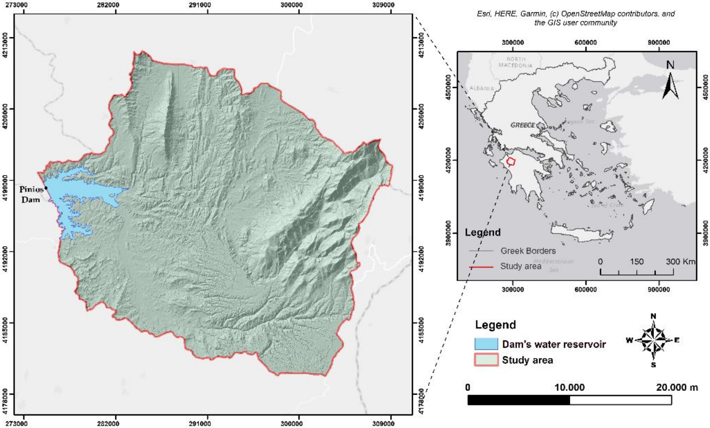
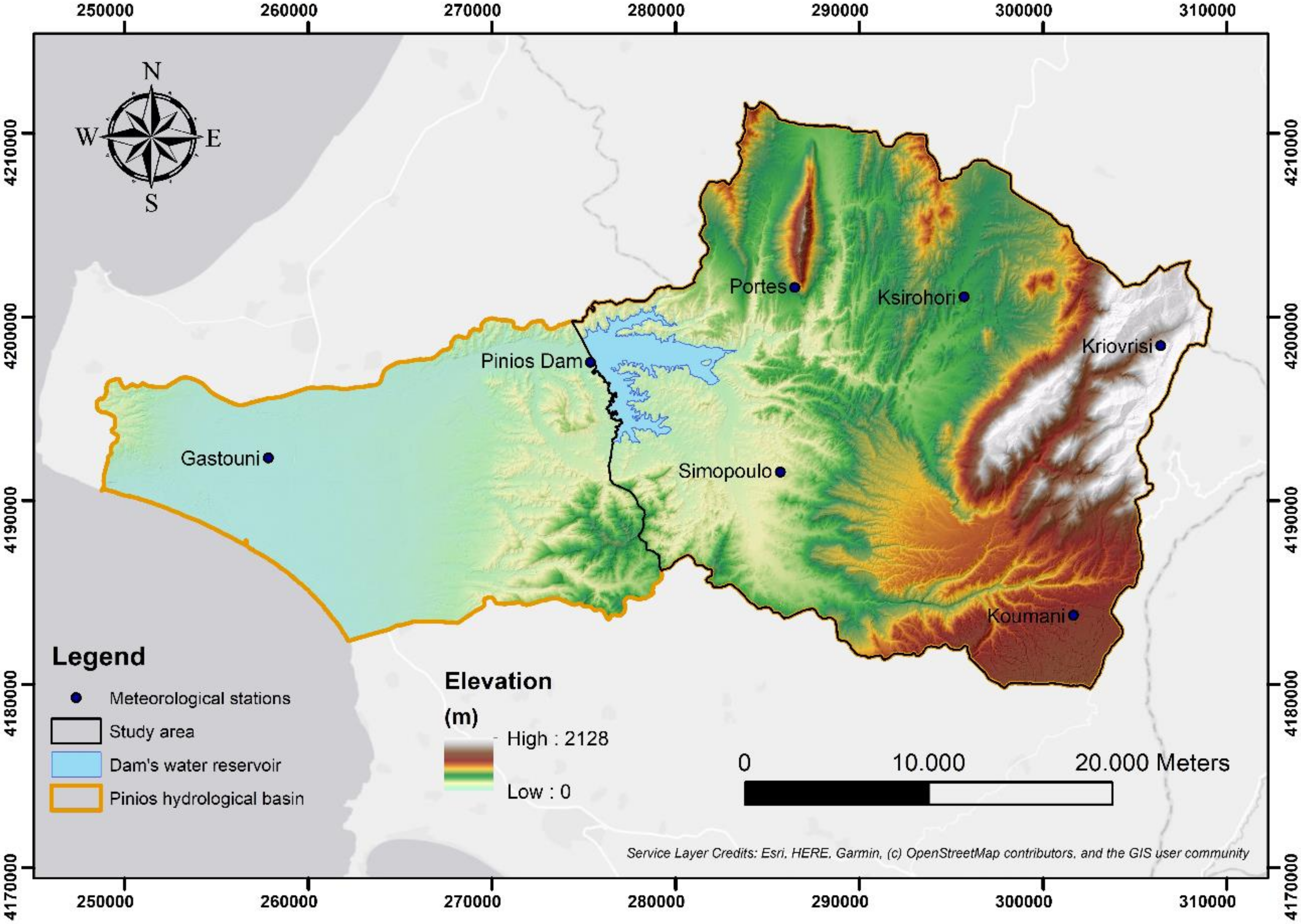
2.1. Research Area

July and August of 2007 in Greece were extremely hot months with hot heat waves and positive temperature anomalies [30]. The hot summer, along with the preceded warm and dry winter, was the main reason, which led to one of the most destructive wildfires nationwide and particularly in the Ilia regional unit, located in western Greece. In this regional unit, approximately 870 km², mainly forest and agricultural land were burned, 63 people were killed, hundreds were injured, and hundreds of houses were destroyed.

The pilot area of research is the drainage basin of the Pinios earth-filled dam, which is located in western Greece and more precisely in the Ilia regional unit. The Pinios river hydrological basin occupies an area of 1026 km², whereas the dam’s drainage basin occupies an area of approximately 700 km² (Figure 1). Surface water run-off from the dam’s drainage basin collects to a large water reservoir that occupies an area of approximately 20 km² [31]. The larger part of the dam’s broader area that was destroyed by the wildfire has been selected as a study (pilot) area for the current research.

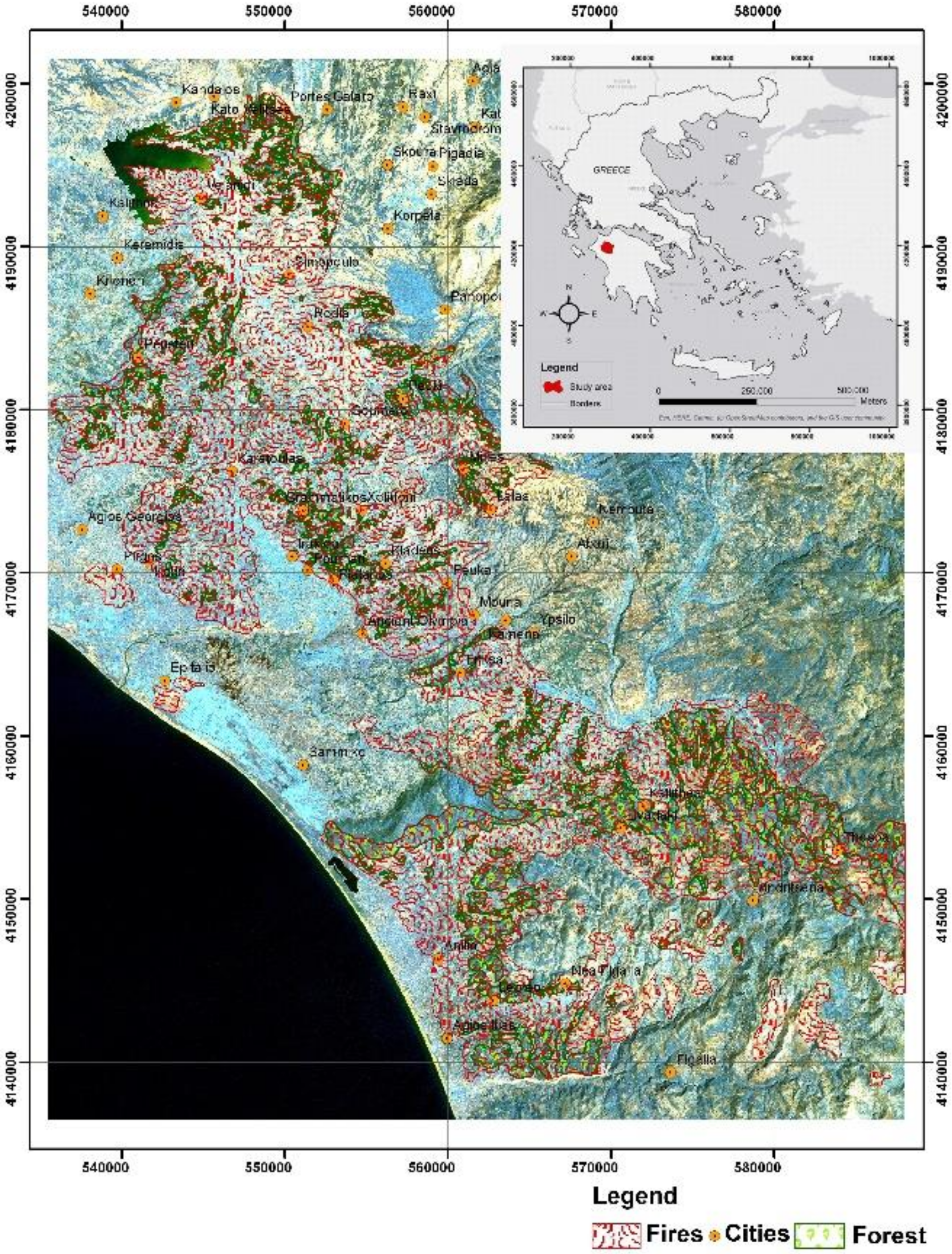
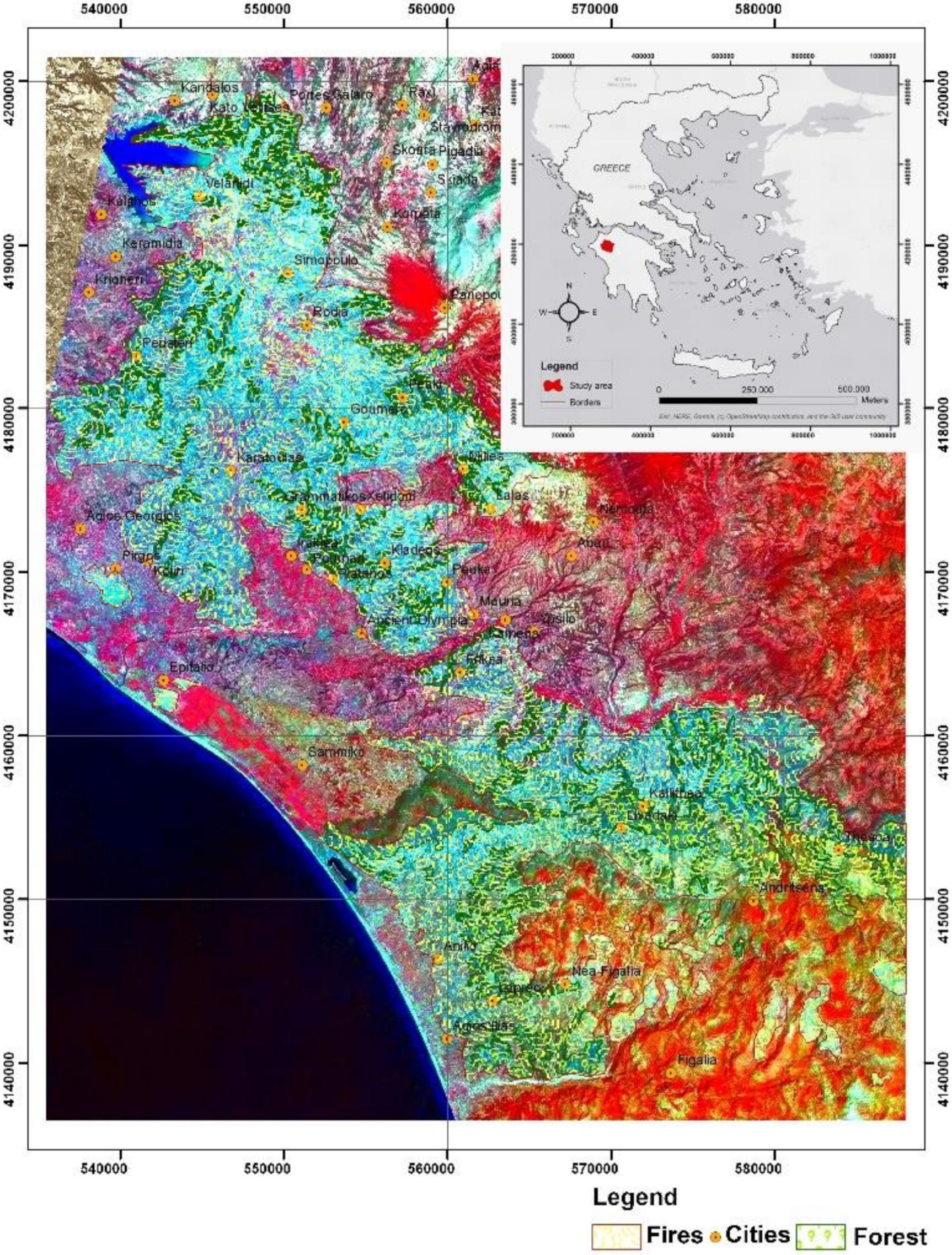
2.2. Satellite Imagery Data

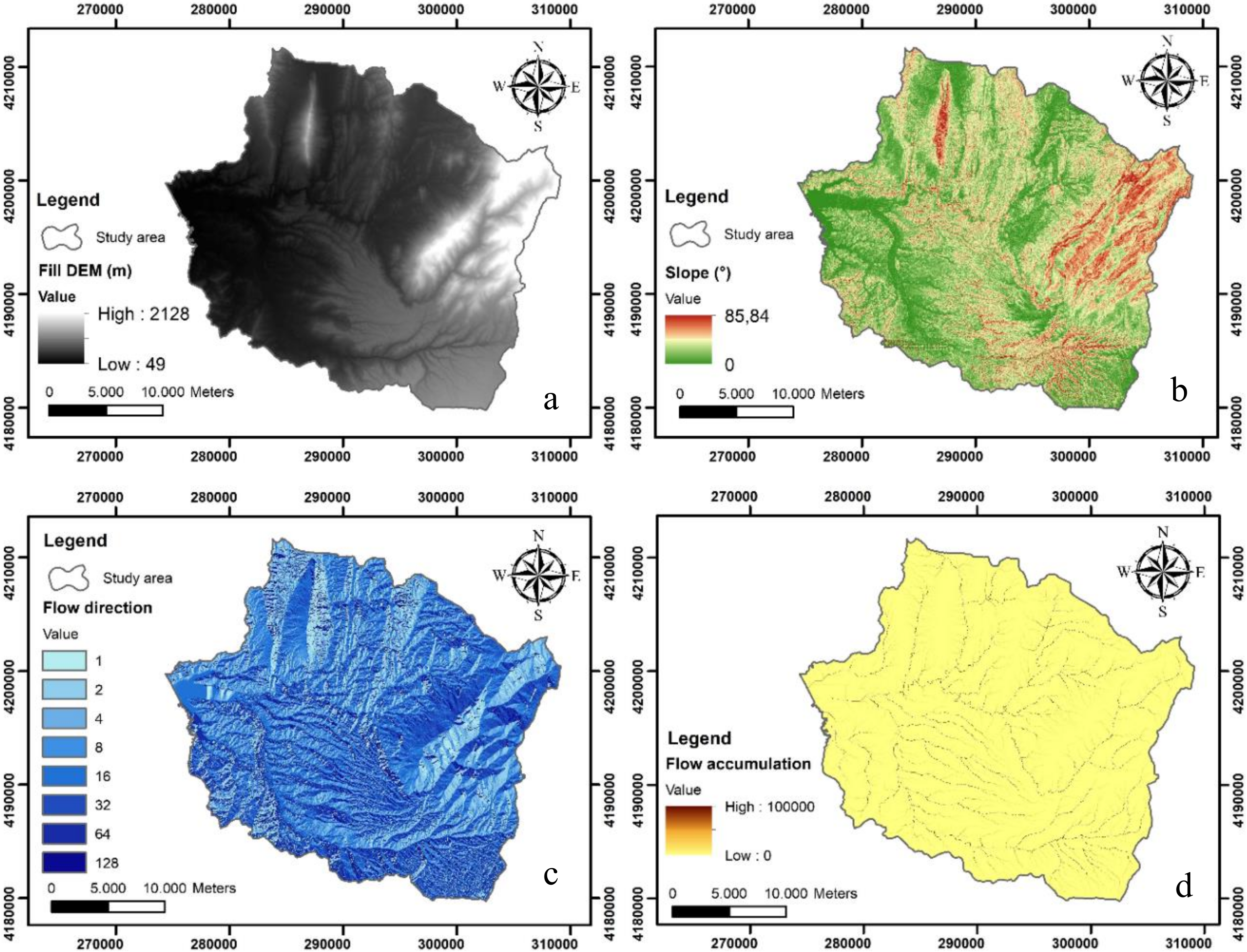
Images acquired from the MODIS radiometer onboard Terra satellite were digitally processed in order to produce vegetation indices before and after the fire event. The total burned area in the Ilia regional unit is estimated as 870 km² by comparing a vegetation index named NDVI (Normalized Difference Vegetation Index) before (10 August 2007) and after (14 September 2007) the wildfire event. The burned area included forest, agricultural and other land, as well as 27 residential areas (mainly villages and settlements), and is presented in a Landsat (Figure 2) and a Spot imagery map (Figure 3), before and after the fire event, respectively. By comparing both maps and satellite data, it was found that 203 km², or 28.93% of the study area, of the drainage basin of the Pinios earth-filled dam, was totally burned.

2.3. Elevation Data

A DΤM (Digital Terrain Model), having a point sampling of 5 m and very high vertical accuracy estimated at 2 m, is used. The DTM is produced by the Greek Cadastral during the two-year period 2007–2009 and covers completely the Greek territory. The source data for the DTM development were colored aerial photos captured by a digital camera onboard an airplane.

From the specific DTM, a Digital Elevation Map (DEM) was produced for the entire hydrological basin of the Pinios river. However, the area of study focuses on the upstream part of the Pinios dam basin (see Figure 4). The necessary analysis of the DEM in a GIS framework led to the development of products such as slope and flow direction maps. In sequence, the specific data set is further processed for the computation of two factors, the slope length (L) and the slope steepness (S) factor.

The coordinate system that was used for georeferencing every map in this study is the Hellenic Geodetic Reference System 1987 (HGRS/EGSA87).

2.4. Rainfall Data

The used rainfall data were derived from seven meteorological stations (Koumani, Kriovrisi, Simopoulo, Ksirohori, Portes, Pinios Dam, Gastouni) that exist in the Pinios hydrological basin (Figure 4). For this purpose, the average annual and monthly rainfalls were calculated for each of the referred stations for a time period of thirty-three years.

2.5. Geology

The surrounding area of the Pinios river basin is structured by Alpine formations of the Greek geotectonic zones of Ionian, Gabrovo-Tripolis and Pindos as well as Quaternary and Neogene deposits. The local geology was surmised by four geological sheets, 1:50,000 in scale (Amalias, Kertezi, Goumeron and Patras), derived from the Hellenic Survey of Geological and Mineral Exploration. The geological formations of these sheets were digitized, imported in a GIS environment and grouped into nine geological categories for the production of a specific geological map of the research area (Figure 5). The nine geological categories were classified according to their lithology, age and permeability.

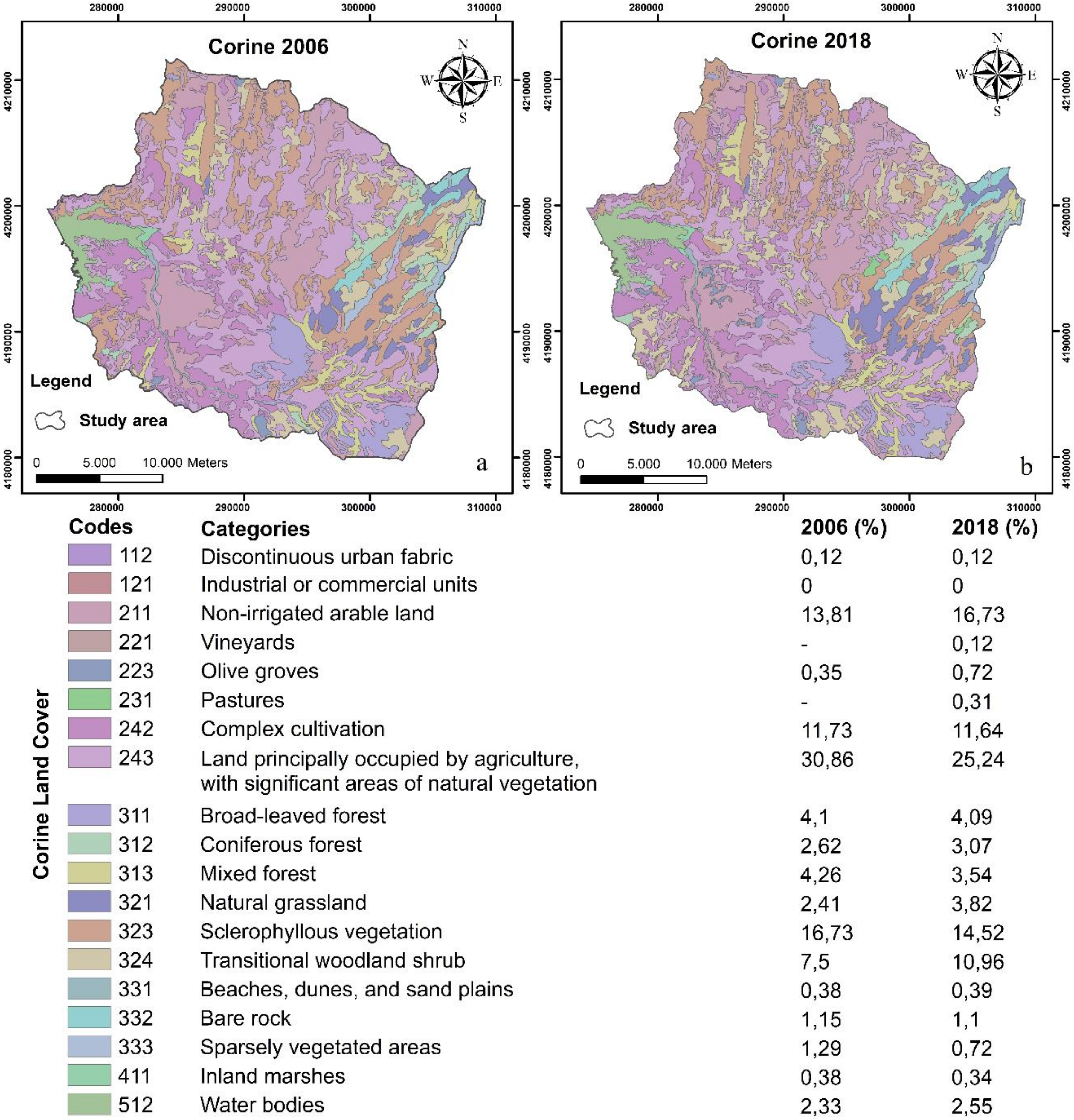
2.6. Corine Land Cover

An important factor affecting soil erosion is vegetation and generally land cover and management. Therefore, it was important to analyze the temporal and spatial variation of land uses in the pilot area. For this purpose, the European Corine Land Cover (CLC) was used and the pilot area was divided into twenty different land use classes, since CLC is one of the most popular and widely used products of the Copernicus Land Monitoring Services program. For the purposes of this research, the Corine 2006 and the Corine 2018 releases (Figure 6) were used in order to estimate the cover management factor (C).

With the use of Arc tools in the GIS environment, it became efficient to produce a CLC table presenting the Land Cover categories and their percentage normalized to the area of study for both the years 2006 and 2018 (Figure 6). The greater extent of the study area was mainly occupied by agricultural land with large areas of natural vegetation, non-irrigated arable land, sclerophyllous vegetation, complex cultivation patterns and transitional woodland shrub. However, the wildfire that broke out in the Ilia regional unit in August 2007 burned a total of 203 km² of land in the pilot area (28.93%) and, as expected, it led to an increment of the soil loss for more than a decade.

3. Factor Analysis and Calculation

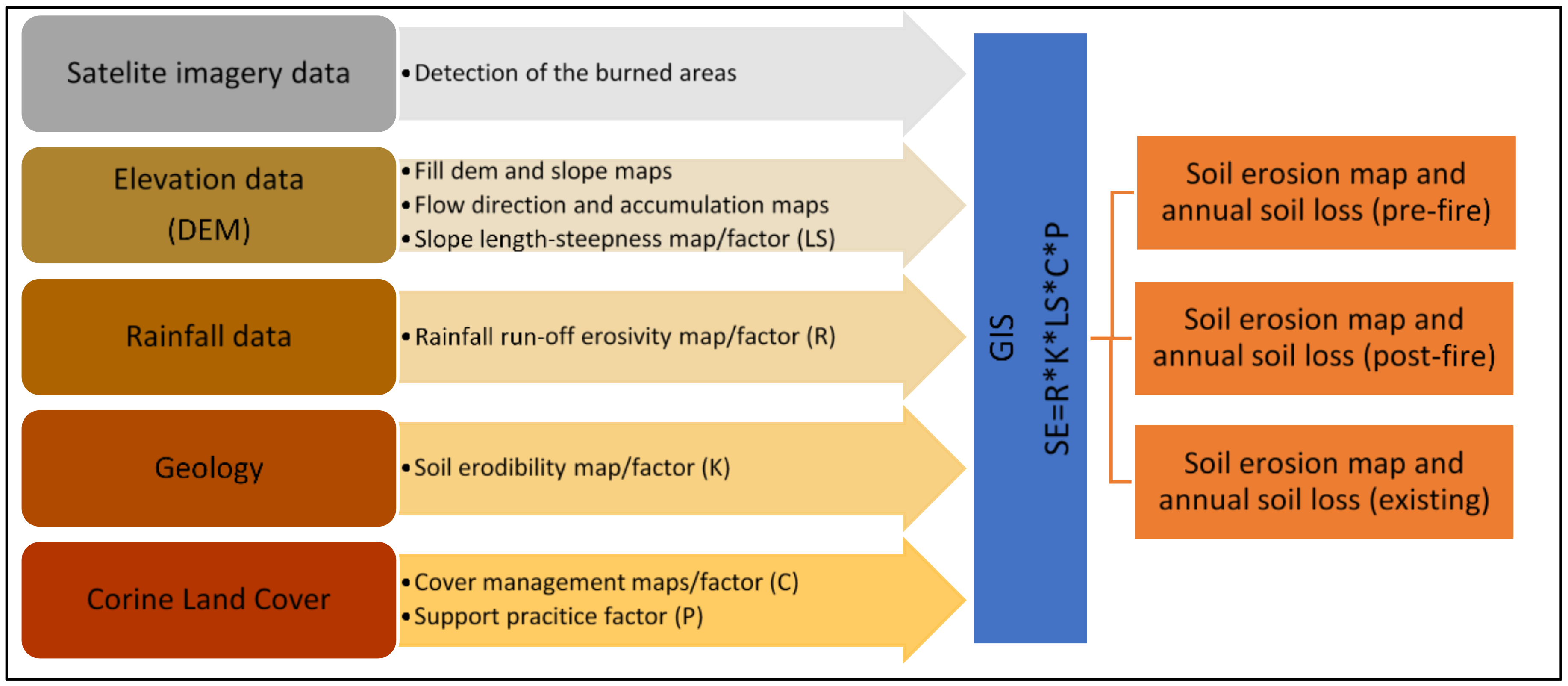
3.1. Methodology

The methodology applied in this research initially consists of the import of all accumulated data in a Geographic Information System (GIS). Consequently, several raster base maps are generated, and all RUSLE factors are calculated. Finally, the RUSLE equation is applied in the GIS and high accuracy soil erosion maps are produced and annual soil loss is calculated at different times (Figure 7).

The computed average soil loss per unit area (SE) is expressed in tons/ha/year, the rainfall-runoff erosivity factor (R) is expressed in MJ mm ha⁻¹ h⁻¹ year, the soil erodibility factor (K) is expressed in t h MJ⁻¹ mm⁻¹. The slope length factor (L), the slope steepness factor (S), the cover management factor (C) and the erosion control practice factor (P) are dimensionless.

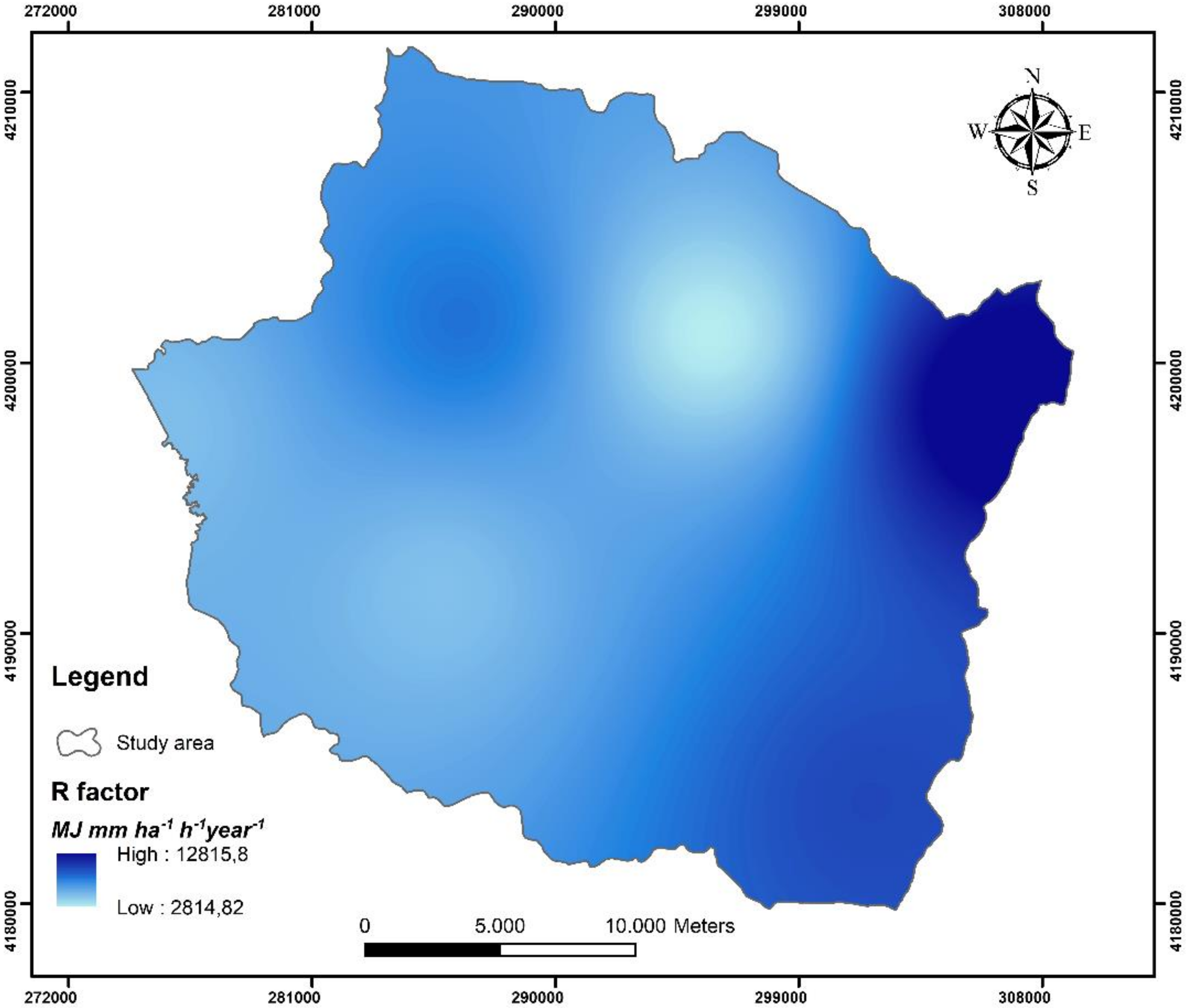
3.2. Rainfall-Runoff Erosivity Factor (R) Analysis and Calculation

Rainfall-runoff erosivity is a term that is used to express the competence of water to cause soil detachment and transport [32] and storm soil losses from cultivated fields that are directly proportional to the value of the storm’s total kinetic energy times its maximum 30-min intensity (EI) [7]. It is represented by the R factor, which is the sum of individual storm EI-values for a year averaged over long time periods (>20 years) to accommodate apparent cyclical rainfall patterns [12]. The difficulty of finding these types of data led to the development of new techniques using different variables that could be more easily measured and quantified and then correlated with the R factor. Fournier’s index [33] is one of them that is generally applied to find a higher correlation between erosivity and soil loss

$$\mathrm{F}={\mathrm{p}}_{\max }{}^2/\mathrm{P}$$

(1)

where p is the average rainfall of the month with the highest rainfall and P is the annual average rainfall.

The most important weakness of this index is that it does not take into consideration the erosive power of rainfalls with low or moderate intensity. Arnoldus [34] modified Fournier’s index by taking into account the rainfall amounts of all months and using the index as an independent variable. As a result, by using the following formula he obtained an improved correlation (r² = 0.83).

$$\mathrm{MF}=\frac{{{\displaystyle \sum }}_{\mathrm{i}=1}^{12}{\mathrm{pi}}^2}{\mathrm{P}}$$

(2)

where MF is the modified Fournier’s index value, Pi is average monthly precipitation, and P is the average annual precipitation.

Following Arnoldus’ [34] work, Renard and Freimund [12] suggested the following formulas for determining the R factor (MJ mm ha⁻¹ h⁻¹ year):

R = 0.7397 * MF^1.847, MF < 55 mm, r² = 0.81

(3)

R = 95.77 − 6.081 * MF + 0.477 * MF², MF > 55 mm, r² = 0.75

The rainfall-runoff erosivity factor R applied in this research was calculated by using the formulas above. The average annual and monthly rainfalls were calculated for each of the meteorological stations existing in the area for a time period of thirty-three years and the calculated R factor imported in a GIS database (

Table 1. The rainfall-runoff erosivity factor (R) around the meteorological stations of the pilot area.

Meteorological Stations	Elevation (m)	Coordinates (X, Y) (HGRS87 Datum *)		Modified Fournier’s Index (mm)	Precipitation (mm)	R Factor (MJ mm ha−1 h−1)
Koumani	500	301,656	4,183,754	144.9	1212	9227
Kriovrisi	950	306,409	4,198,446	169.8	1482.9	12,816
Simopoulo	211	285,702	4,191,557	102.5	847.3	4485
Ksirohori	291	295,710	4,201,094	82.1	722.9	2815
Portes	300	286,485	4,201,604	132.6	660.2	7676
Pinios Dam	82	275,361	4,197,535	103.8	783.8	4600
Gastouni	5	257,834	4,192,331	107.4	801.3	4947

Notes: * Hellenic Geodetic Reference System 1987 datum.

).

By using the Geostatistical Analyst toolbox of the GIS software and after several trial tests of spatial distribution it was concluded that the best method for the spatial distribution of (R) factor mend was the Inverse Distance Weighting (IDW). The Inverse Distance Weighting is a deterministic method of spatial interference which produces a continuous surface using only the geometric features of point measurements. The R factor that was estimated with this method is presented in the following map of R distribution (Figure 8). Rainfall-runoff erosivity factor R map of the pilot area.).

Dark blue color represents areas with a higher R factor, whereas white color represents areas with a lower R factor. From the data interpretation, it is concluded that in higher altitudes the R factor gets higher, especially in the eastern part of the pilot area. By using the GIS toolboxes, the average rainfall-runoff erosivity factor (R) in the pilot area was calculated to be equal to 6609.47 MJ mm ha⁻¹ h⁻¹ year⁻¹, with a maximum and minimum value of 12,815.83 and 2814.82 MJ mm ha⁻¹ h⁻¹ year⁻¹, respectively.

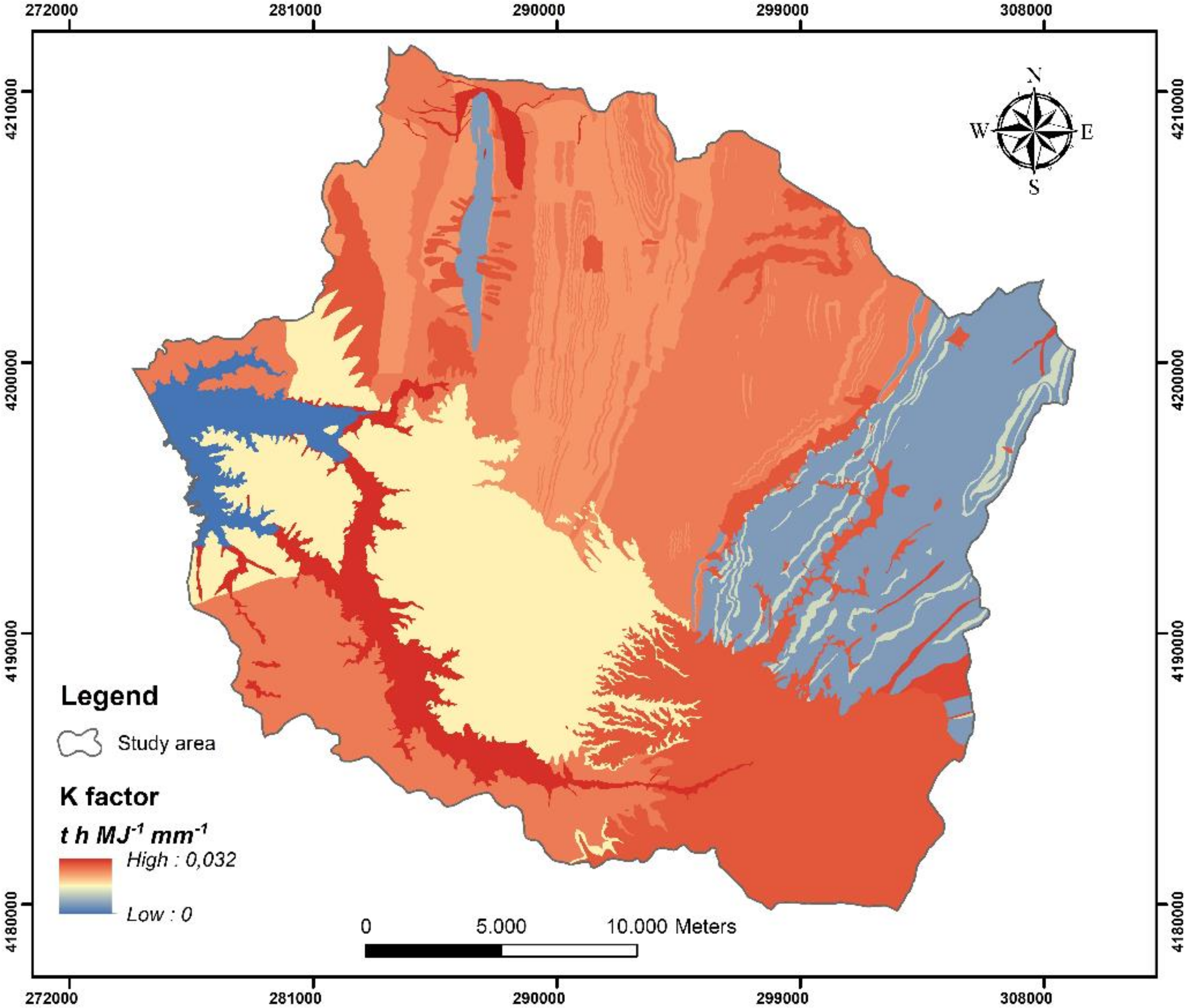
3.3. Soil Erodibility Factor (K) Analysis and Calculation

Erodibility, as a term, is the measure of the susceptibility of soils for detachment and transport due to the elements of erosion [32]. Soils erode in varying degrees due to their properties, regardless of the current conditions such as land slope, rainfall, land cover and management. The susceptibility of soil to erosion, the sediment transportability and the amount and rate of runoff in each rainfall expresses the loss of soil per unit of R [ton/ha per unit R] [13]. In this study, soil erodibility is associated with the erosion susceptibility of geological formations. The correlation (between soil erodibility and erosion susceptibility arises from the fact that geological formations can be divided into many different categories depending on their sensitivity to physical and chemical weathering and their ability to produce sediments.

The geological formations prevailing in the pilot area were classified according to their lithology, age, and permeability into nine categories and the ArcMap software was used to estimate the soil erodibility factor in each of the nine geological categories (

Table 2. Erodibility factors (K) of the geological formations prevailing in the pilot area.

Geological Formations	K (t.h/MJ mm)
Quaternary deposits	0.032
Pleistocene coarse deposits	0.029
Plio–Pleistocene coarse deposits	0.027
Plio–Pleistocene fine deposits	0.018
Flysch with sandstones	0.024
Flysch with siltstones	0.027
Flysch basement	0.031
Transition zone (cherts, sandstones and siltstones)	0.012
Limestones	0.005

and Figure 9) by using the methodology and the following equations presented by Wischmeier and Smith [7,8].

K = [(2.1M^1.14 (10⁻⁴)(12 − a) + 3.25(b − 2) + 2.5(c − 3))/100]

(4)

M = Ps × (100 − Pc)

where K is the soil erodibility factor (t ha h ha⁻¹ MJ⁻¹ mm⁻¹), M is the grain size parameter, a is the organic matter content (%), b is the structure index, c is the permeability index, Ps (%) is the “silt & very fine sand” fraction content and Pc (%) is the clay fraction content and the erodibility factor is multiplied with the number 0.1317 in order to transform its units to t.h/MJ mm [7,35].

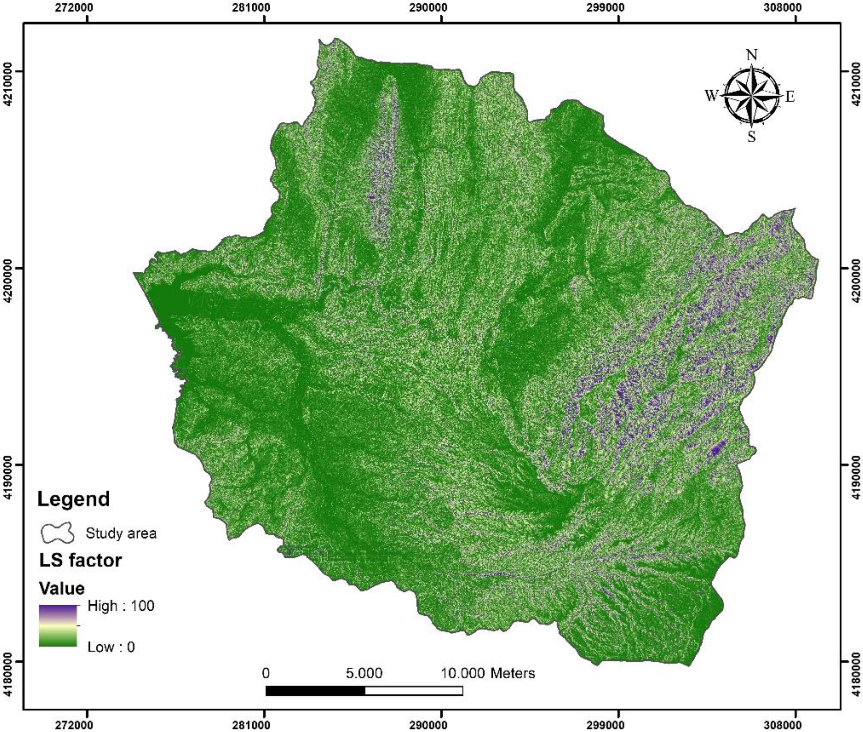
3.4. Slope Length and Steepness Factor (LS) Analysis and Calculation

LS is a combination of the slope length factor L and the slope gradient factor S, which reflects the effect of the slope length and steepness on the soil erosion process. The slope-length factor (L) is the ratio of soil loss (A) from a field slope length to that from a slope 22.1 m long. It measures the distance from the origin of overland flow along the flow path to the location of deposition. The slope-steepness factor (S) is the ratio of soil erosion from the field slope gradient to that from a 9% slope [8]. The LS factor is generally estimated by applying the following equation:

LS = (A/22.13)^m(sinβ/0.09)ⁿ

(5)

which has been widely used and partly modified by several researchers of this topic [36,37,38].

Digital Elevation Models (DEMs), accompanied by the use of satellite data and GIS, have an important role in the investigation of soil erosion since they can be used in the precise identification of the terrain features [39,40]. Each DEM grid cell contains a value corresponding to its actual elevation on the Earth’s surface [41] and the computation of the LS factor is highly dependent on the DEM accuracy [42]. In this research, a DEM with 5 m accuracy (Figure 4) was used and the following equation [38] was imported in the GIS to estimate the distribution of the LS factor in the area of study.

LS = (m+1)(A/22.13)^m(sinβ/0.09)ⁿ

(6)

where A is the upslope contributing area per unit width of contour (m²/m), β is the slope angle, m is an exponent varying from 0.4 to 0.6 and n is an exponent varying from 1 to 1.3. Thus, 22.13 m and 0.09 in the denominator refer to the length and slope of the standard unit plot, respectively.

The DEM that was created for the area of study (Figure 4), as well as the above formula, was imported into the ArcMap software, and with the appropriate processing all the necessary maps were produced (Figure 10), in which each cell size received a value of 5 equal to the DEM’s accuracy.

From the LS map interpretation (Figure 11), it is evident that its highest values were identified in the eastern part of the research area where mountains and river gorges exist. On the contrary, the lower LS values occur in the western part of the research area, where the slope relief is smoother. With the use of the appropriate Arc tools, it was estimated that the average topographic factor (LS) is equal to 7.5.

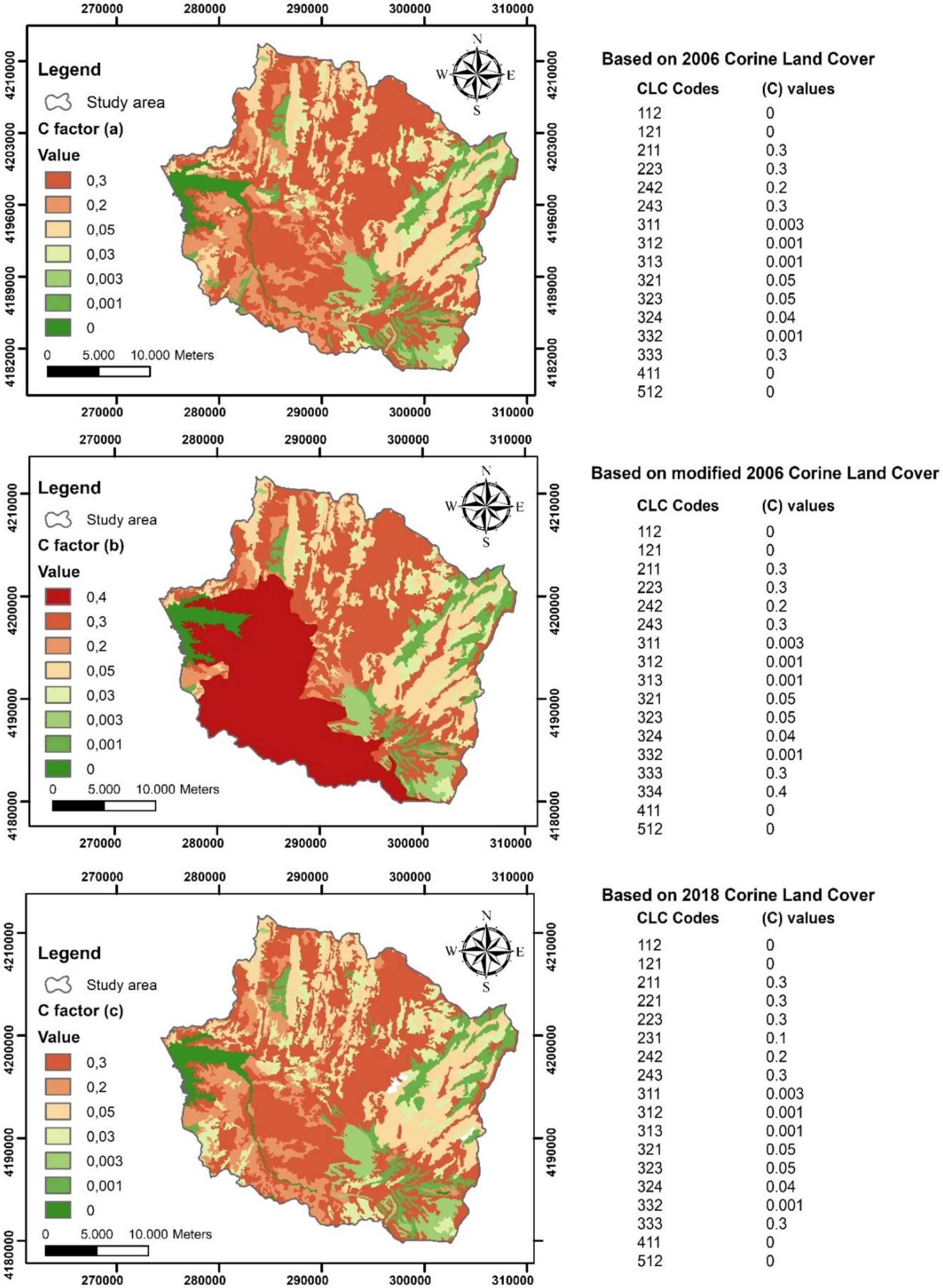
3.5. Cover Management Factor (C) Analysis and Calculation

Vegetation is a natural filter existing above the soil which absorbs some of the energy of falling raindrops, wind and running water, so that less is transported into the soil, while the root vegetation system contributes to the mechanical strength of the soil [43]. After topography, the vegetation cover is the most important factor that controls soil erosion [44].

Generally, the C factor ranges between 1 and 0. In the first case, no cover is presented and the ground surface is considered to be similar to barren land, whereas a very thick cover means a well-protected soil, with C values near zero (0) [45]. In order to calculate the C factor in the area of study, the Corine Land Cover (CLC) database was used (Figure 6). Each land use category from CLC was matched with the corresponding bibliographic values of C factor [46,47,48,49,50] and the cover management map in the pilot area was finally generated with the use of GIS. At the end, three cover management factor (C) maps were produced (Figure 12). The first map represents the C factor before the wildfire, the second map the C factor after the wildfire and the third map the C factor a decade after the wildfire. It should be noted that the area with a CLC code 334 corresponds to the burned land and receives a value of 0.4 as it has been suggested by other researchers [46,47,48,49,50,51].

3.6. Support Practice Factor (P) Analysis and Calculation

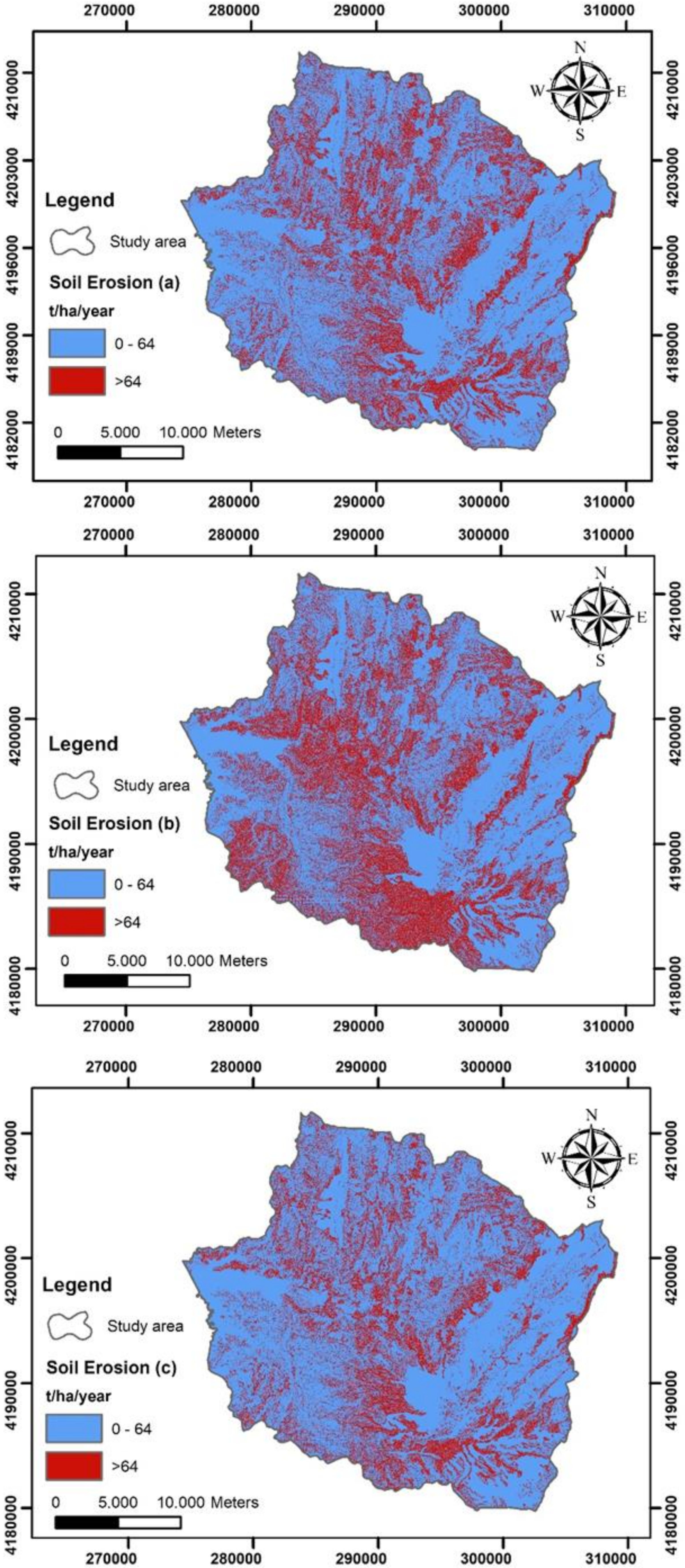
The support practice factor P is the ratio of soil loss, affected by an explicit support practice, to the corresponding loss with upslope and downslope cultivation [13]. This type of practice affects erosion by modifying the flow pattern and the direction of surface runoff and by reducing the amount and rate of surface runoff [51]. Some of the most important support practices are the contour cultivation, the contour strip cropping and the terrace systems [8]. The P factor is dimensionless, and its values range from 0 to 1. Values close to zero point out that support measures against erosion have been taken in the area while values close to 1 correspond to the worst cases where no support measures have been implemented. It is practically impossible to get the value zero because erosion cannot be prevented but can only be slowed down using support practices. In most cases, the P factor is set directly to 1 due to the absence of data on the management practices implemented in the study areas. However, this approach does not take into consideration the inhibitory effect of practices in the area. According to Shin [52], these practices on cultivated lands (contour, cropping, and terrace) are crucial factors that can control erosion.

In the area of study, a high percentage of land is devoted to agricultural practices such as olive groves, cultivation patterns, non-irrigated arable land, and land mainly occupied by agriculture with a lot of areas of natural vegetation. Furthermore, some individual protection measures have been implemented without detailed data being available [50]. Agricultural and forest land (CLC codes: 211, 221, 223, 231, 242, 243) account for 56.74% of the total area, which is too high to ignore the impact of crop systems on soil erosion. Thus, the P factor was set to 0.5. This value was chosen considering that nearly 50% of the total area is devoted to agricultural areas such as olive groves, meadows, vineyards, compound crops, non-irrigated arable land, as well as areas mainly occupied by agriculture with significant natural vegetation.

4. Results

Based on the factor analysis and calculation presented in the previous paragraphs, and with the use of the RUSLE equation imported in the GIS framework, annual soil erosion maps are finally produced. Specifically, the Raster Calculator command is executed in the ArcMap environment where all the relevant RUSLE factors are multiplied by each other. The result of this procedure is the development of a new raster file representing the soil loss in the area of study.

Three maps of different annual soil erosion are produced with this process. The first map is related to the soil erosion condition that existed before the wildfire incident, the second map is related to the post-fire soil erosion condition and the third map reflects the existing soil erosion condition (Figure 13). All values of soil erosion are referred in tons per hectare per year (t/ha/year). High values are presented with a red color and low values with a blue color.

By comparing the three generated maps, it is evident that there is a significant increase in erosion on the second map which is even more evident in the western part of the research area. In general, high values of soil loss occur in areas with high terrain and steep slopes as well as along streams. The effect of rainfall, in this case, is also significant because the values of the rainfall erosivity factor are high enough to exacerbate soil erosion. On the other hand, the role of vegetation and land cover is more important because the burned land proved to be the most vulnerable to erosion.

The mean annual soil loss arises automatically calculated from the available statistics existing in the ArcMap program. The pre-fire mean annual soil loss is equal to SE₍₁₎ = 69 t/ha/year (Figure 13a) and the corresponding value of soil loss immediately after the wildfire is SE₍₂₎ = 94 t/ha/year (Figure 13b). Finally, based on existing and recent conditions, a decade after the wildfire, the mean annual soil loss value is equal to SE₍₃₎ = 64 t/ha/year (Figure 13c).

The most important element from the above process is mainly the estimation of changes in the percentage of soil loss and the factors that affect it. More specifically, the rate of increase in soil erosion immediately after the fire event is found to be equal to 36.2%, with an average increase in the C factor by 28%. After a decade since the fire event, the rate of reduction in soil loss is found to be equal to 31%, with a corresponding reduction in the C factor by 26%, which reflects the physical rehabilitation of the area.

5. Discussion

Soil loss is an important environmental problem, responsible for a series of non-reversible environmental disturbances, being linked with desertification processes. Even though soil erosion rate is being estimated by a series of different models, its spatial distribution comprises a quite complex task since it is closely linked to vegetation type, presenting great variability from year to year. Especially when wildfires occur, things are getting worse.

Scientists have developed several erosion models worldwide, based mainly on statistical relations between a series of parameters [3,4]. Rainfall, topography, vegetation cover, runoff, and soil erodibility, are some of them. The empirical RUSLE model also constitutes an important tool for land use and post-fire erosion estimations. Even though the RUSLE model has been widely used [11,12,13], there are limited data regarding the ground erosion rate changes over the years when a wildfire has occurred, and in which extend the cover management factor controls’ soil loss.

The methodology applied in this research is based on the empirical RUSLE model and the import of its factors in a GIS environment. With this methodology, the generation of high accuracy soil erosion maps in areas that have suffered severe soil loss changes due to wildfires is evident and soil loss can be calculated over time. In more detail, in the drainage basin of the Pinios earth-filled dam (pilot area), it was calculated that 28.93% of burned vegetation reflects a soil loss rate increase of 36.2%. After a decade of physical rehabilitation, soil loss rate reaches the same rate as it had before the fire event.

All these must be taken seriously into account since soil erosion prevention strategies are mainly based on the construction of costly manmade structures although vegetation and its quick reclamation in burned areas may effectively prevent erosion processes.

The main challenge of the proposed methodology and the exported model is to produce reliable results, depending on the quality and quantity of the inserted data, in order to simulate different scenarios from different catchments and visualize them with the export of appropriate maps. Thus, the model must be tested in different field conditions in order to estimate its accuracy. Furthermore, the exported model may be linked to a Decision Support System (DSS), aiming at a complete proposal for a sustainable and efficient environmental management of catchments that have been affected by extreme wildfires or other natural disasters.

6. Conclusions

The aim of this study is to present a method calculating the ground erosion rates for post- and pre-wildfire conditions and to produce the necessary model maps to compare pre-fire and post-fire soil erosion changes at different time intervals. For this purpose, it imports the factors of the RUSLE equation in a Geographic Information System (GIS) and generates, with the appropriate analysis, soil erosion maps of high accuracy. Soil erosion rate changes, in areas affected by wildfires, then can be easily calculated at different time intervals.

The model maps that are produced because of this methodology are compared with each other by collating average annual soil erosion maps and rates before the fire, immediately after the fire and for the existing conditions. This type of map generation is applied on a detailed Digital Elevation Model (DEM). Very important is also the utilization of high-resolution satellite imagery data for the detection of the burned areas as well as the assessment of the severity of fire to the factors used in the RUSLE equation.

The most important element in this process is the accurate estimation of soil erosion changes in the affected areas. In the pilot area, the drainage basin of the Pinios earth-filled dam located in the Ilia Regional Unit, the rate of increase in soil erosion rate immediately after the fire event was found to be equal to 36.2%, with an average increase in the C factor by 28%. After a decade since the fire event, the rate of reduction in soil loss was found to be equal to 31%, with a corresponding reduction in the C factor by 26%, which reflects the physical rehabilitation of the area. A significant amount of this soil loss has been deposited in the dam’s reservoir, which in the end may cause aggradation and reduction in the dam’s operational life, thus needing further investigation.

References

1. EC PESETA II Project: Projection of the Economic Impact of Climate Change in Sectors of the European Union Based on Bottom-Up Analysis. Available online: https://ec.europa.eu/jrc/en/peseta (accessed on 15 November 2019).
2. Vieira, D.C.S.; Serpa, D.; Nunes, J.P.C.; Prats, S.A.; Neves, R.; Keizer, J.J. Predicting the effectiveness of different mulching techniques in reducing post-fire runoff and erosion at plot scale with the RUSLE, MMF and PESERA models. Environ. Res. 2018, 165, 365–378. [Google Scholar] [CrossRef] [PubMed]
3. Varela, M.E.; Benito, E.; Keijer, J.J. Wildfire effects on soil erodibility of woodlands in NW Spain. Land Degrad. Dev. 2010, 21, 75–82. [Google Scholar] [CrossRef]
4. Moody, J.A.; Shakesby, R.A.; Robichaud, P.R.; Cannon, S.H.; Martin, D.A. Current research issues related to post-wildfire runoff and erosion processes. Earth Sci. Rev. 2013, 122, 10–37. [Google Scholar] [CrossRef]
5. Richter, G. Aspects and problems of soil erosion hazard in the EEC countries. In Soil Erosion; Prendergast, A.G., Ed.; Commission of the European Communities: Report No. EUR 8427 EN.1983; Office for Official Publications of the European Communities: Luxembourg, 1983; pp. 9–17. [Google Scholar]
6. Robichaud, R.P.; Cerdà, A. (Eds.) Summary and Remarks. In Chapter 21: Fire Effects on Soils and Restoration Strategies; Science Publishers: Enfield, NH, USA, 2009. [Google Scholar]
7. Wischmeier, W.H.; Smith, D.D. Predicting Rainfall-Erosion Losses from Cropland East of the Rocky Mountains; Agriculture Handbook No. 282; US Department of Agriculture: Washington, DC, USA, 1965.
8. Wischmeier, W.H.; Smith, D.D. Predicting Rainfall Erosion Losses, a Guide to Conservation Planning; Agriculture Handbook No. 537; US Department of Agriculture, Science and Education Administration: Washington, DC, USA, 1978.
9. Wischmeier, W.H. Estimating the soil loss equation’s cover and management factor for undisturbed area. In Present and Prospective Technology for Predicting Sediment Yields and Sources; USDA ARS Publication ARS-S: Washington, DC, USA, 1975; Volume 40, pp. 118–124. [Google Scholar]
10. Kinnell, P.I.A.; Risse, L.M. USLE-M: Empirical modelling rainfall erosion through runoff and sediment concentration. Soil Sci. Soc. Am. J. 1998, 62, 1667–1672. [Google Scholar] [CrossRef]
11. Renard, K.G.; Foster, G.R.; Weesies, G.A.; Porter, J.P. Revised universal soil loss equation. J. Soil Water Conserv. 1991, 46, 30–33. [Google Scholar]
12. Renard, K.G.; Freimund, J.R. Using Monthly Precipitation Data to Estimate the R Factor in the Revised USLE. J. Hydrol. 1994, 157, 287–306. [Google Scholar] [CrossRef]
13. Renard, K.G.; Foster, G.R.; Weesies, G.A.; McCool, D.K.; Yoder, D.C. Predicting Soil Erosion by Water: A Guide to Conservation Planning with the Revised Universal Soil Loss Equation (RUSLE); Agriculture Handbook, No.703. USDA-ARS; United States Department of Agriculture: Washington, DC, USA, 1997; p. 384.
14. Lopez-Vicente, M.; Navas, A. Predicting Soil Erosion with RUSLE in Mediterranean Agricultural Systems at Catchment Scale. Soil Sci. 2009, 174, 272–282. [Google Scholar] [CrossRef] [Green Version]
15. Morgan, R.P.C.; Quinton, J.N.; Smith, R.E.; Govers, G.; Poesen, J.W.A.; Auerswald, K.; Chisci, G.; Torri, D.; Styczen, M.E. The European Soil Erosion Model (EUROSEM): A dynamic approach for predicting sediment transport from fields and small catchments. Earth Surf. Process. Landf. 1998, 23, 527–544. [Google Scholar] [CrossRef]
16. Mati, B.M.; Morgan, R.P.C.; Quinton, J.N. Soil erosion modelling with EUROSEM at Embori and Mukogodo catchments, Kenya. Earth Surf. Process. Landf. 2006, 35, 579–588. [Google Scholar] [CrossRef] [Green Version]
17. Kirkby, M.; Gobin, A.; Irvine, B. Pan European Soil Erosion Risk Assessment. In Deliverable 5: PESERA Model Strategy, Land Use and Vegetation Growth; European Soil Bureau: Brussels, Belgium, 2003; Available online: http://eusoils.jrc.it/ (accessed on 23 June 2019).
18. Kirkby, M.J.; Irvine, B.J.; Jones, R.J.A.; Govers, G.; PESERA Team. The PESERA coarse scale erosion model for Europe. Model rationale and implementation. Eur. J. Soil Sci. 2008, 59, 1293–1306. [Google Scholar] [CrossRef]
19. Alexakis, D.D.; Hadjimitsis, D.G.; Agapiou, A. Integrated use of remote sensing, GIS and precipitation data for the assessment of soil erosion rate in the catchment area of “Yialias” in Cyprus. Atmos. Res. 2013, 131, 108–124. [Google Scholar] [CrossRef]
20. Borrelli, P.; Märker, M.; Panagos, P.; Schütt, B. Modeling soil erosion and river sediment yield for an intermountain drainage basin of the Central Apennines, Italy. CATENA 2014, 114, 45–58. [Google Scholar] [CrossRef]
21. Phinzi, K.; Ngetar, N.S. The assessment of water-borne erosion at catchment level using GIS-based RUSLE and remote sensing: A review. Int. Soil Water Conserv. Res. 2018, 7, 27–46. [Google Scholar] [CrossRef]
22. Di Piazza, G.V.; Di Stefano, C.; Ferro, V. Modelling the effects of a bushfire on erosion in a Mediterranean basin/Modélisation des impacts d’un incendie sur l’érosion dans un bassin Méditerranéen. Hydrol. Sci. J. 2007, 52, 1253–1270. [Google Scholar] [CrossRef]
23. Fernandez, C.; Vega, J.A.; Vieira, D.C.S. Assessing soil erosion after fire and rehabilitation treatments in NW Spain: Performance of rusle and revised Morgan–Morgan–Finney models. Land Degrad. Dev. 2010, 21, 58–67. [Google Scholar] [CrossRef] [Green Version]
24. Rulli, M.C.; Offeddu, L.; Santini, M. Modeling post-fire water erosion mitigation strategies. Hydrol. Earth Syst. Sci. 2013, 17, 2323–2337. [Google Scholar] [CrossRef] [Green Version]
25. Efthimiou, N.; Psomiadis, E.; Panagos, P. Fire severity and soil erosion susceptibility mapping using multi-temporal Earth Observation data: The case of Mati fatal wildfire in Eastern Attica, Greece. CATENA 2020, 187, 1–16. [Google Scholar] [CrossRef]
26. Esteves, T.C.J.; Kirkby, M.J.; Shakesby, R.A.; Ferreira, A.J.D.; Soares, J.; Irvine, B.; Ferreira, C.S.S.; Coehlo, C.O.A.; Bento, C.P.M.; Carreira, M. Mitigating land degradation caused by wildfire: Application of the PESERA model to fire-affected sites in central Portugal. Geoderma 2012, 191, 40–50. [Google Scholar] [CrossRef]
27. Karamesouti, M.; Petropoulos, G.P.; Papanikolaou, I.D.; Kairis, O.; Kosmas, K. Erosion rate predictions from PESERA and RUSLE at a Mediterranean site before and after a wildfire: Comparison & implications. Geoderma 2016, 261, 44–58. [Google Scholar]
28. Fernandez, C.; Vega, J.A. Evaluation of the rusle and disturbed wepp erosion models for predicting soil loss in the first year after wildfire in NW Spain. Environ. Res. 2018, 165, 279–285. [Google Scholar] [CrossRef]
29. Myronidis, D.; Arabatzis, G. Evaluation of greek post-fire erosion mitigation policy through spatial analysis. Pol. J. Environ. Stud. 2009, 18, 865–872. [Google Scholar]
30. Founda, D.; Giannakopoulos, C. The exceptionally hot summer of 2007 in Athens, Greece—A typical summer in the future climate? Glob. Planet. Chang. 2009, 67, 227–236, E-ISSN: 2224-3496. [Google Scholar] [CrossRef]
31. Depountis, N.; Vidali, M.; Kavoura, K.; Sabatakakis, N. Soil erosion prediction at the water reservoir’s basin of Pineios dam, Western Greece, using the Revised Universal Soil Loss Equation (RUSLE) and GIS. WSEAS Trans. Environ. Dev. 2018, 14, 457–463, E-ISSN: 2224-3496. [Google Scholar]
32. Lal, R.; Soil and Water Conservation Society (U.S.). Soil Erosion: Research Methods, 2nd ed.; Soil and Water Conservation Society: Delray Beach, FL, USA; St. Lucie Press: Ankeny, IA, USA, 1994. [Google Scholar]
33. Fournier, F. Climat et Erosion; Presses Universitaires de France: Paris, France, 1960. [Google Scholar]
34. Arnoldus, H.M.J. Methodology used to determine the maximum potential average annual soil loss due to sheet and rill erosion in Morocco. FAO Soil Bull. 1977, 34, 39–48. [Google Scholar]
35. Foster, G.R.; McCool, D.K.; Renard, K.G.; Moldenhauer, W.C. Conversion of the Universal Soil Loss Equation to SI metric units. J. Soil Water Conserv. 1981, 36, 355–359. [Google Scholar]
36. Moore, I.D.; Burch, G.J. Physical basis of the length-slope factor in the Universal Soil Loss Equation. Soil Sci. Soc. Am. J. 1986, 50, 1294–1298. [Google Scholar] [CrossRef]
37. Moore, I.D.; Wilson, J.P. Length-slope factors for the Revised Universal Soil Loss Equation: Simplified method of estimation. J. Soil Water Conserv. 1992, 4, 423–428. [Google Scholar]
38. Mitasova, H.; Mitas, L. Multiscale soil erosion simulations for land use management. In Landscape Erosion and Evolution Modeling; Harmon, R.S., Doe, W.W., III, Eds.; Springer: New York, NY, USA, 2001; pp. 321–347. [Google Scholar] [CrossRef]
39. Holmes, K.; Chadwick, O.; Kyriakidis, P. Error in a USGS 30-m digital elevation model and its impact on terrain modeling. J. Hydrol. 2000, 233, 154–173. [Google Scholar] [CrossRef]
40. Raj, A.R.; George, J.; Raghavendra, S.; Kumar, S.; Agrawal, S. Effect of DEM resolution on LS factor computation. Int. Arch. Photogramm. Remote Sens. Spat. Inf. Sci 2018, XLII-5, 315–321. [Google Scholar] [CrossRef] [Green Version]
41. Khosrowpanah, S.; Heitz, L.; Wen, Y.; Park, M. Developing a GIS-based Soil Erosion Potential Model of the Ugum Watershed; Technical Report No. 117; Water Environmental Research Institute of the Western Pacfic, University of Guam: Mangilao, Guam, 2007. [Google Scholar]
42. Liu, H.; Kiesel, J.; Hörmann, G.; Fohrer, N. Effects of DEM horizontal resolution and methods on calculating the slope length factor in gently rolling landscapes. CATENA 2011, 87, 368–375. [Google Scholar] [CrossRef]
43. Morgan, R.P.C. Soil Erosion and Conservation, 3rd ed.; Blackwell Publishing Co.: Malden, MA, USA, 2005. [Google Scholar]
44. Van der Knijff, J.M.; Jones, R.J.A.; Montanarella, L. Soil Erosion Risk Assessment in Europe, JRC Scientific and Technical Report—EUR 19022 EN; European Soil Bureau, European Commission: Brussels, Belgium, 2000; 58p. [Google Scholar]
45. Pham, T.G.; Degener, J.; Kappas, M. Integrated universal soil loss equation (USLE) and Geographical Information System (GIS) for soil erosion estimation in A Sap basin: Central Vietnam. Int. Soil Water Conserv. Res. 2018, 6. [Google Scholar] [CrossRef]
46. Bakker, M.; Gover, G.; Doorn, A.; Quetier, F.; Chouvardas, D.; Rounsevell, M. The response of soil erosion and sediment export to land-use change in four areas of Europe: The importance of landscape pattern. Geomorphology 2008, 98, 213–226. [Google Scholar] [CrossRef]
47. Diodato, N.; Fagnano, M.; Alberico, I. Geospatial and visual modeling for exploring sediment source areas across the Sele river landscape, Italy. Ital. J. Agron. 2011, 6, e14. [Google Scholar] [CrossRef]
48. Panagos, P.; Borrelli, P.; Meusburger, K.; Alewell, C.; Lugato, E.; Montanarella, L. Estimating the soil erosion cover-management factor at the European scale. The new assessment of soil loss by water erosion in Europe. Land Use Policy 2015, 48, 38–50. [Google Scholar] [CrossRef]
49. Xanthakis, M. Soil Erosion Study at Mountainous Basin of Marathon’s Lake, Attica Greece, Using Modern Technological Tools. Ph.D. Thesis, Harokopio Panepistimio of Athens, Kallithea, Greece, 2011; 288p. [Google Scholar]
50. Vidali, M. Estimation of Soil Erosion Model in the Reservoir of the Pinios Dam of Ilia Prefecture. Master’s Thesis, University of Patras, Patras, Greece, 2013; 114p. [Google Scholar]
51. Renard, K.G.; Foster, G.R. Soil conservation: Principles of erosion by water. In Dryland Agriculture; Dregne, H.E., Willis, W.O., Eds.; American Society of Agronomy: Madison, WI, USA, 1983; pp. 155–176. [Google Scholar]
52. Shin, G.J. The Analysis of Soil Erosion Analysis in the Watershed Using GIS. Ph.D. Thesis, Gang-won National University, Chuncheon, Korea, 1999. [Google Scholar]
Figure 1. Pilot area.
Ijgi 09 00562 g001
Figure 2. The burned area presented in a Landsat imagery map.
Ijgi 09 00562 g002
Figure 3. The burned area presented in a Spot imagery map.
Ijgi 09 00562 g003
Figure 4. Digital Elevation Map (DEM) of the pilot area.
Ijgi 09 00562 g004
Figure 5. Geological map of the pilot area.
Ijgi 09 00562 g005
Figure 6. (a) Corine Land Cover 2006 map and (b) Corine Land Cover 2018 map of the pilot area.
Ijgi 09 00562 g006
Figure 7. Presentation of the applied methodology.
Ijgi 09 00562 g007
Figure 8. Rainfall-runoff erosivity factor R map of the pilot area.
Ijgi 09 00562 g008
Figure 9. Soil erodibility factor (K) map of the pilot area.
Ijgi 09 00562 g009
Figure 10. (a) Fill DEM map, (b) slope map, (c) flow direction map, (d) flow accumulation map.
Ijgi 09 00562 g010
Figure 11. Slope length and steepness factor (LS) map of the pilot area.
Ijgi 09 00562 g011
Figure 12. Cover management factor maps of the pilot area (a) before the wildfire, (b) after the wildfire and (c) a decade after the wildfire.
Ijgi 09 00562 g012
Figure 13. (a) Pre-fire soil erosion, (b) post-fire soil erosion, (c) existing soil erosion—maps of the research area.
Ijgi 09 00562 g013