Integrative Analysis of Spatial Heterogeneity and Overdispersion of Crime with a Geographically Weighted Negative Binomial Model


Abstract
1. Introduction
2. Data and Methods
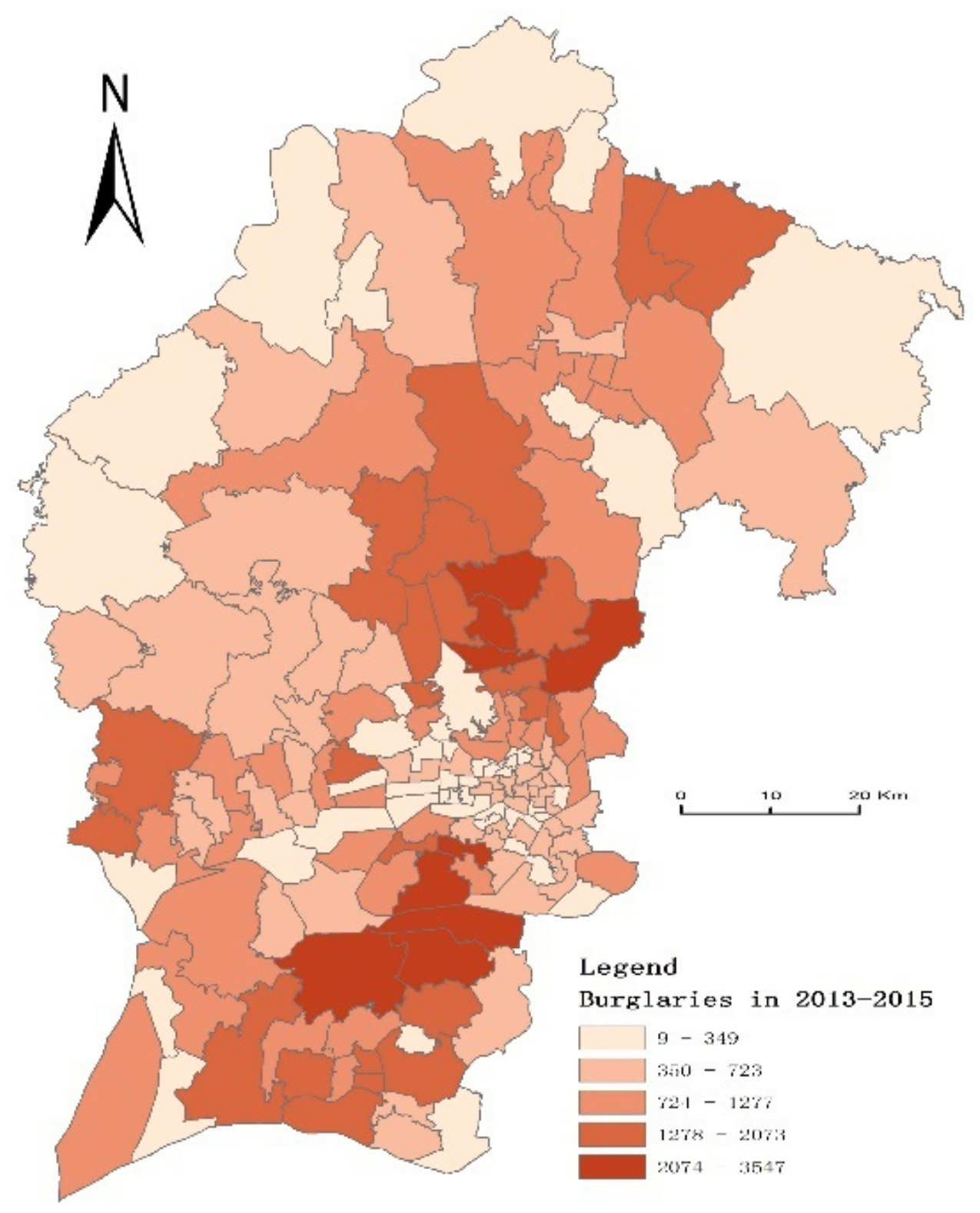
2.1. Study Area
2.2. Data
2.3. Methodology
2.3.1. Negative Binomial Model (NB)
2.3.2. Geographically Weighted Poisson Model (GWPR)
2.3.3. Geographically Weighted Negative Binomial Model (GWNBR)
3. Results and Discussion
3.1. Model Performance Comparison
3.2. Parameters Estimation
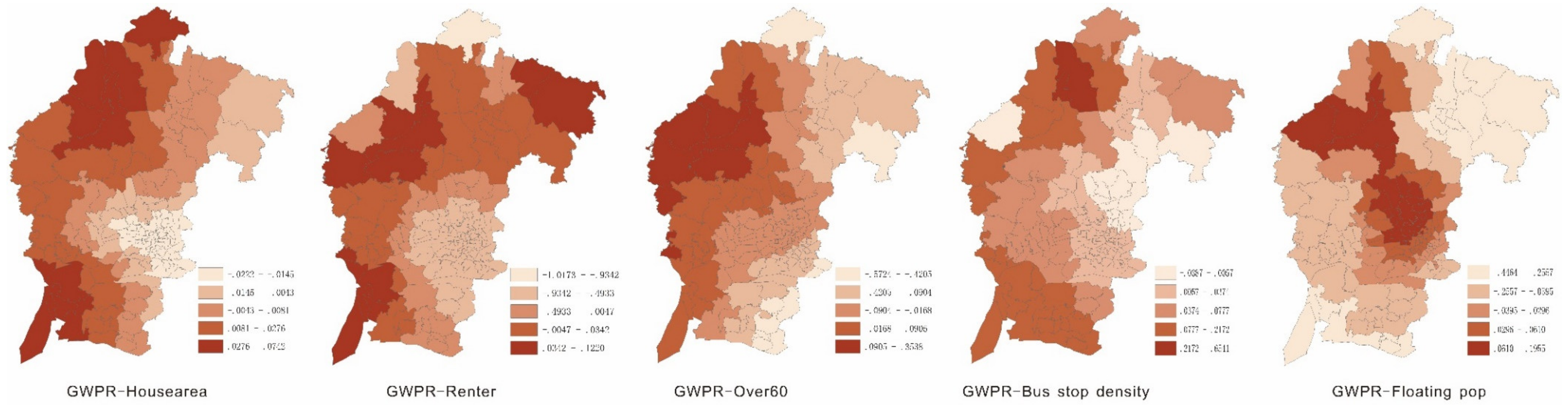
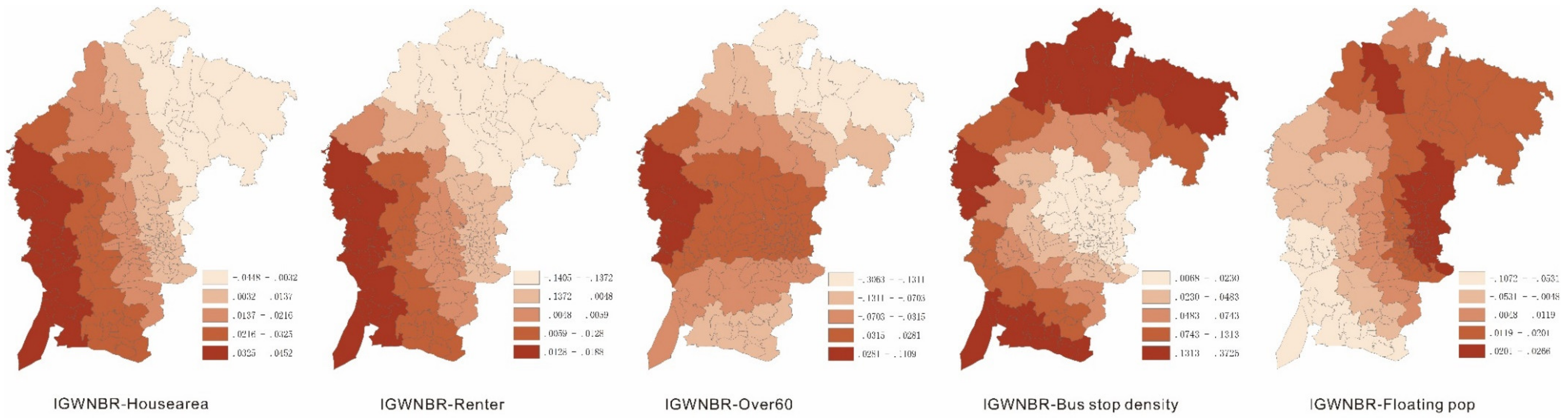
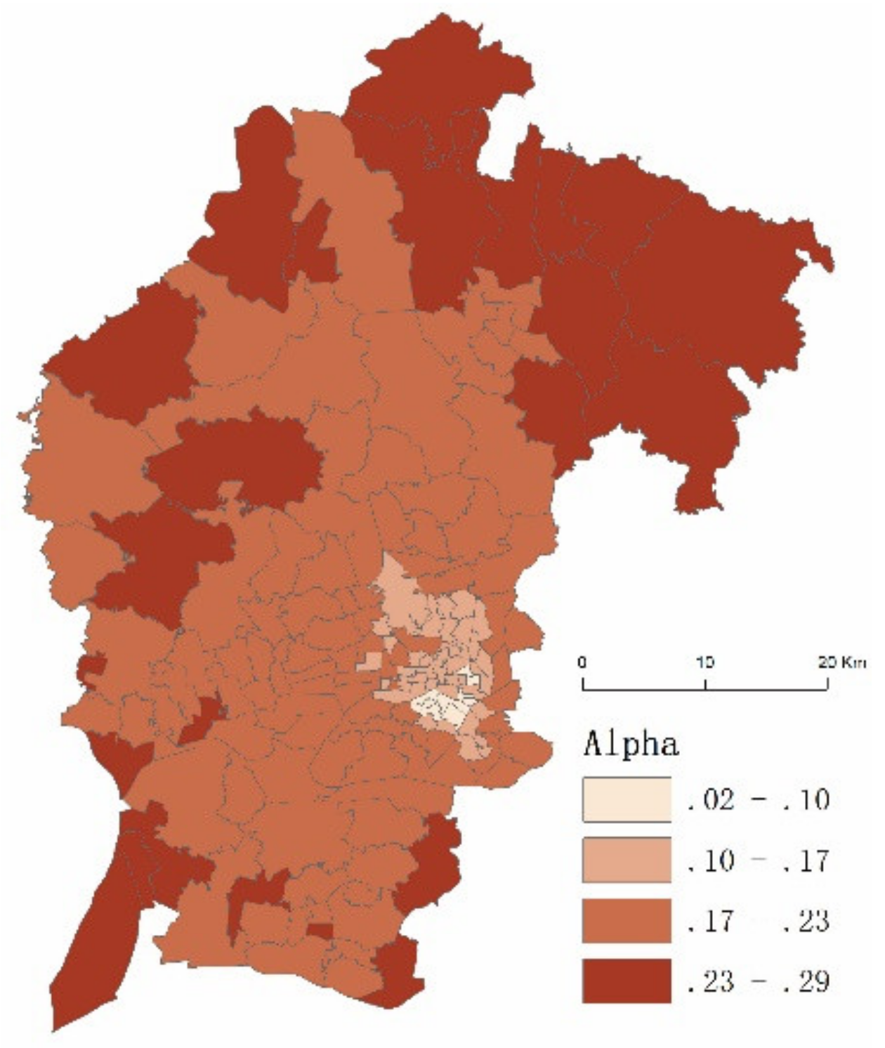
3.3. Spatial Analyses of the Coefficients
3.4. Limitations
4. Conclusions
Author Contributions
Funding
Acknowledgments
Conflicts of Interest
References
- Uittenbogaard, A.; Ceccato, V. Space-time Clusters of Crime in Stockholm, Sweden. Rev. Eur. Stud. 2012, 4, 148–156. [Google Scholar] [CrossRef]
- Zhang, C.; Peterson, M. A spatial analysis of neighborhood crime in Omaha, Nebraska using alternative measures of crime rates. Int. J. Criminol. 2007, 31, 1–28. [Google Scholar]
- Breetzke, G.D. Modeling violent crime rates: A test of social disorganization in the city of Tshwane, South Africa. J Crim. Justice 2010, 38, 446–452. [Google Scholar] [CrossRef]
- Melo, S.N.D.; Andresen, M.A.; Matias, L.F. Geography of crime in a Brazilian context: An application of social disorganization theory. Urban Geogr. 2017, 38, 1550–1572. [Google Scholar] [CrossRef]
- Shi, S.; Dong, Y.; Song, L. A spatio-temporal analysis of urban crime in Beijing: Based on data for property crime. Urban Stud. 2015, 53, 3223–3245. [Google Scholar]
- Cohen, L.E.; Felson, M. Social change and crime rate trends: A routine activity approach. Am. Sociol. Rev. 1979, 44, 588–608. [Google Scholar] [CrossRef]
- Brantingham, P.; Brantingham, P. Crime pattern theory. Environ. Criminol. Crime Anal. 2013, 78–93. [Google Scholar] [CrossRef]
- Shaw, C.R.; Mckay, H.D. Juvenile delinquency and urban areas. Soc. Serv. Rev. 1942, 35, 394. [Google Scholar] [CrossRef]
- Liu, H.; Zhu, X. Exploring the Influence of Neighborhood Characteristics on Burglary Risks: A Bayesian Random Effects Modeling Approach. ISPRS Int. J. Geo Inf. 2016, 5, 102. [Google Scholar] [CrossRef]
- Warner, B.D.; Pierce, G.L. Reexamining Social Disorganization Theory Using Calls to the Police as a measure of crime*. Criminology 1993, 31, 493–517. [Google Scholar] [CrossRef]
- Grubesic, T.H.; Mack, E.A.; Kaylen, M.T. Comparative modeling approaches for understanding urban violence. Soc. Sci. Res. 2012, 41, 92–109. [Google Scholar] [CrossRef] [PubMed]
- Paternoster, R.; Brame, R.; Bachman, R.; Sherman, L.W. Do fair procedures matter? The effect of procedural justice on spouse assault. Law Soc. Rev. 1997, 31, 163–204. [Google Scholar] [CrossRef]
- Song, G.; Liu, L.; Bernasco, W.; Zhou, S.; Xiao, L.; Long, D. Theft from the person in urban China: Assessing the diurnal effects of opportunity and social ecology. Habitat Int. 2018, 78, 13–20. [Google Scholar] [CrossRef]
- Zhou, H.; Liu, L.; Lan, M.; Yang, B.; Wang, Z. Assessing the Impact of Nightlight Gradients on Street Robbery and Burglary in Cincinnati of Ohio State, USA. Remote Sens. 2019, 11, 1958. [Google Scholar] [CrossRef]
- Lan, M.; Liu, L.; Hernandez, A.; Liu, W.; Zhou, H.; Wang, Z. The Spillover Effect of Geotagged Tweets as a Measure of Ambient Population for Theft Crime. Sustainability 2019, 11, 6748. [Google Scholar] [CrossRef]
- Brunsdon, C.; Fotheringham, A.S.; Charlton, M.E. Geographically Weighted Regression: A Method for Exploring Spatial Nonstationarity. Geogr. Anal. 1996, 28, 281–298. [Google Scholar] [CrossRef]
- Murillo, F.H.S.; Chica-Olmo, J. The spatial heterogeneity of factors of feminicide: The case of Antioquia-Colombia. Appl. Geogr. 2018, 92, 63–73. [Google Scholar] [CrossRef]
- Zhang, H.; Mccord, E.S. A spatial analysis of the impact of housing foreclosures on residential burglary. Appl. Geogr. 2014, 54, 27–34. [Google Scholar] [CrossRef]
- Mburu, L.W.; Helbich, M. Crime Risk Estimation with a Commuter-Harmonized Ambient Population. Ann. Assoc. Am. Geogr. 2016, 106, 804–818. [Google Scholar] [CrossRef]
- Helbich, M.; Arsanjani, J.J. Spatial eigenvector filtering for spatiotemporal crime mapping and spatial crime analysis. Cartogr. Geogr. Inf. Sci. 2015, 42, 134–148. [Google Scholar] [CrossRef]
- Chun, Y. Analyzing space–time crime incidents using eigenvector spatial filtering: An application to vehicle burglary. Geogr. Anal. 2014, 46, 165–184. [Google Scholar] [CrossRef]
- Law, J.; Quick, M. Exploring links between juvenile offenders and social disorganization at a large map scale: A Bayesian spatial modeling approach. J. Geogr. Syst. 2013, 15, 89–113. [Google Scholar] [CrossRef]
- Law, J. Bayesian Spatial Random Effect Modelling for Analysing Burglary Risks Controlling for Offender, Socioeconomic, and Unknown Risk Factors. Appl. Spat. Anal. Policy 2012, 5, 73–96. [Google Scholar] [CrossRef]
- Chen, J.; Liu, L.; Zhou, S.; Xiao, L.; Jiang, C. Spatial variation relationship between floating population and residential burglary: A case study from, Z.G.; China. ISPRS Int. J. Geo Inf. 2017, 6, 246. [Google Scholar] [CrossRef]
- Chen, J.; Liu, L.; Zhou, S.; Xiao, L.; Song, G.; Ren, F. Modeling spatial effect in residential burglary: A case study from ZG city, China. ISPRS Int. J. Geo Inf. 2017, 6, 138. [Google Scholar] [CrossRef]
- Park, S.M.; Tark, J.; Cho, Y.I. Victimization immunity and lifestyle: A comparative study of over-dispersed burglary victimizations in South Korea and, U.S. Int. J. Law Crime Justice 2016, 45, 44–58. [Google Scholar] [CrossRef]
- Hope, T.; Norris, P.A. Heterogeneity in the Frequency Distribution of Crime Victimization. J. Quant. Criminol. 2013, 29, 543–578. [Google Scholar] [CrossRef][Green Version]
- Yang, Z.; Hardin, J.W.; Addy, C.L. A score test for overdispersion in Poisson regression based on the generalized Poisson-2 model. J. Stat. Plan. Inference 2009, 139, 1514–1521. [Google Scholar] [CrossRef]
- Song, G.; Lin, L.; Bernasco, W.; Xiao, L.; Zhou, S.; Liao, W. Testing Indicators of Risk Populations for Theft from the Person across Space and Time: The Significance of Mobility and Outdoor Activity. Ann. Am. Assoc. Geogr. 2018, 108, 1370–1388. [Google Scholar] [CrossRef]
- Berk, R.; MacDonald, J.M. Overdispersion and Poisson regression. J. Quant. Criminol. 2008, 24, 269–284. [Google Scholar] [CrossRef]
- Bottcher, J.; Ezell, M.E. Examining the effectiveness of boot camps: A randomized experiment with a long-term follow up. J Res Crime Delinq 2005, 42, 309–332. [Google Scholar] [CrossRef]
- Gomes, M.J.T.L.; Cunto, F.; Silva, A.R. Geographically weighted negative binomial regression applied to zonal level safety performance models. Accid. Anal. Prev. 2017, 106, 254. [Google Scholar] [CrossRef] [PubMed]
- Da Silva, A.R.; Rodrigues, T.C.V. Geographically weighted negative binomial regression—Incorporating overdispersion. Stat. Comput. 2014, 24, 769–783. [Google Scholar] [CrossRef]
- CSY. China Statistical Yearbook; China Statistical Publishing House: Beijing, China, 2016. [Google Scholar]
- Sohn, D.W. Residential crimes and neighbourhood built environment: Assessing the effectiveness of crime prevention through environmental design (CPTED). Cities 2016, 52, 86–93. [Google Scholar] [CrossRef]
- Katz, C.M.; Wallace, D.; Hedberg, E.C. A Longitudinal Assessment of the Impact of Foreclosure on Neighborhood Crime. J. Res. Crime Delinq. 2011, 50, 359–389. [Google Scholar] [CrossRef]
- Malczewski, J.; Poetz, A. Residential Burglaries and Neighborhood Socioeconomic Context in London, Ontario: Global and Local Regression Analysis*. Prof. Geogr. 2005, 57, 516–529. [Google Scholar] [CrossRef]
- Ariel, B.; Partridge, H. Predictable Policing: Measuring the Crime Control Benefits of Hotspots Policing at Bus Stops. J. Quant. Criminol. 2016, 33, 809–833. [Google Scholar] [CrossRef]
- Hunter, J.; Tseloni, A. Equity, justice and the crime drop: The case of burglary in England and Wales. Crime Sci. 2016, 5, 1–13. [Google Scholar] [CrossRef]
- Lee, J.; Park, S.; Jung, S. Effect of Crime Prevention through Environmental Design (CPTED) Measures on Active Living and Fear of Crime. Sustainability 2016, 8, 872. [Google Scholar] [CrossRef]
- Nobles, M.R.; Ward, J.T.; Tillyer, R. The Impact of Neighborhood Context on Spatiotemporal Patterns of Burglary. J. Res. Crime Delinq. 2016, 53, 711–740. [Google Scholar] [CrossRef]
- Osgood, D.W.; Chambers, J.M. Social Disorganization outside the Metropolis: An analysis of rural youth violence*. Criminology 2000, 38, 81–116. [Google Scholar] [CrossRef]
- Nagin, D.S.; Land, K.C. Age, Criminal Careers, and Population Heterogeneity: Specification and Estimation of a Nonparametric, Mixed Poisson Model*. Criminology 1993, 31, 327–362. [Google Scholar] [CrossRef]
- Xu, P.; Huang, H. Modeling crash spatial heterogeneity: Random parameter versus geographically weighting. Accid. Anal. Prev. 2015, 75, 16–25. [Google Scholar] [CrossRef] [PubMed]
- Nakaya, T.; Charlton, M.; Lewis, P.; Fortheringham, S.; Brunsdon, C. Windows Application for Geographically Weighted Regression Modelling; Ritsumeikan University: Kyoto, Japan, 2012. [Google Scholar]
- Tobler, W.R. A Computer Movie Simulating Urban Growth in the Detroit Region. Econ. Geogr. 1970, 46, 234–240. [Google Scholar] [CrossRef]
- Curran, D.J. Economic reform, the floating population, and crime: The transformation of social control in China. J. Contemp. Crim. Justice 1998, 14, 262–280. [Google Scholar] [CrossRef]
- Situ, Y.; Liu, W. Transient population, crime, and solution: The Chinese experience. Int. J. Offender Ther. 1996, 40, 293–299. [Google Scholar] [CrossRef]
- Hadayeghi, A.; Shalaby, A.S.; Persaud, B.N. Development of planning level transportation safety tools using Geographically Weighted Poisson Regression. Accid. Anal. Prev. 2010, 42, 676–688. [Google Scholar] [CrossRef]
- Kooi, B.R. Assessing the correlation between bus stop densities and residential crime typologies. Crime Prev. Commun. Saf. 2013, 15, 81–105. [Google Scholar] [CrossRef]
- Beavon, D.J.; Brantingham, P.L.; Brantingham, P.J. The influence of street networks on the patterning of property offenses. Crime Prev. Stud. 1994, 2, 115–148. [Google Scholar]
- White, G.F. Neighborhood permeability and burglary rates. Justice Q. 1990, 7, 57–67. [Google Scholar] [CrossRef]
- Lee, S. Spatial Analyses of Installation Patterns and Characteristics of Residential Burglar Alarms. J. Appl. Secur. Res. 2011, 6, 82–109. [Google Scholar] [CrossRef]
- Hillier, B. Can streets be made safe? Urban Des. Int. 2004, 9, 31–45. [Google Scholar] [CrossRef]
- Shu, C.F. Housing layout and crime vulnerability. Urban Des. Int. 2000, 5, 177–188. [Google Scholar]
- Lin, L.; Chao, J.; Zhou, S.; Kai, L.; Du, F. Impact of public bus system on spatial burglary patterns in a Chinese urban context. Appl. Geogr. 2017, 89, 142–149. [Google Scholar]
- Chang, D. Social crime or spatial crime? Exploring the effects of social, economical, and spatial factors on burglary rates. Environ. Behav. 2011, 43, 26–52. [Google Scholar] [CrossRef]
- Ratcliffe, J.H.; McCullagh, M.J. Hotbeds of crime and the search for spatial accuracy. J. Geogr. Syst. 1999, 1, 385–398. [Google Scholar] [CrossRef]
- Ratcliffe, J.H. Detecting Spatial Movement of Intra-Region Crime Patterns Over Time. J. Quant. Criminol. 2005, 21, 103–123. [Google Scholar] [CrossRef]
- Hay, G.; Marceau, D.; Dube, P.; Bouchard, A. A multiscale framework for landscape analysis: Object-specific analysis and upscaling. Landsc. Ecol. 2001, 16, 471–490. [Google Scholar] [CrossRef]
- Lechner, A.M.; Langford, W.T.; Jones, S.D.; Bekessy, S.A.; Gordon, A. Investigating species–environment relationships at multiple scales: Differentiating between intrinsic scale and the modifiable areal unit problem. Ecol. Complex. 2012, 11, 91–102. [Google Scholar] [CrossRef]


| Variables | Definition | Mean | Min | Max | STD |
|---|---|---|---|---|---|
| Dependent variable | |||||
| Residential burglaries | Total number of residential burglaries per police station management areas (PSMA) | 698.2 | 9 | 3547 | 668.17 |
| Explanatory variable | |||||
| House area | Percent of household with house area equal to or greater than 120 m2 (%) | 21.865 | 0 | 72.3 | 16.502 |
| Renter | Percent of people who pay rent for the use of a room (%) | 29.02 | 0.2 | 87.7 | 21.655 |
| Over60 | Percent of people over 60 years of age (%) | 9.483 | 0.3 | 19.3 | 4.282 |
| Bus stop density | Number of bus stop/area | 4.343 | 0 | 18.71 | 4.128 |
| Floating population | Percent of floating population from another province (%) | 21.695 | 0.462 | 73.617 | 15.795 |
| House Area | Renter | Over 60 | Bus Stop Density | Floating Population | |
|---|---|---|---|---|---|
| House area | 1 | ||||
| Renter | −0.54 ** | 1 | |||
| Over60 | −0.142 | −0.447 ** | 1 | ||
| Bus stop density | −0.483 ** | 0.17 * | 0.393 ** | 1 | |
| Floating population | −0.113 | 0.667 ** | −0.623 ** | −0.204 ** | 1 |
| Bandwidth | RMSE | 2LL | AICc | |
|---|---|---|---|---|
| NB | --- | 423.53 | −1489.195 | 2992.389 |
| GWPR | 6.334 | 326.49 | −1396.358 | 3217.286 |
| global GWNBR | 20.603 | 378.8 | −1458.856 | 2954.412 |
| local GWNBR | 12.469 | 351.43 | −1434.415 | --- |
| Model | Moran’s I | p-Value |
|---|---|---|
| NB | 0.054 | 0.000 |
| GWPR | −0.028 | 0.000 |
| global GWNBR | 0.012 | 0.070 |
| local GWNBR | 0.004 | 0.829 |
| Variable | NB | GWPR | Global GWNBR | Local GWNBR | |||||||||||||||
|---|---|---|---|---|---|---|---|---|---|---|---|---|---|---|---|---|---|---|---|
| Mean | Min | Lwr | Median | Upr | Max | Mean | Min | Lwr | Med | Upr | Max | Mean | Min | Lwr | Med | Upr | Max | ||
| Intercept | −4.421 | 3.684 | −4.467 | 3.236 | 4.012 | 4.688 | 11.429 | −4.266 | −5.547 | −4.359 | −4.165 | −4.086 | −3.281 | −4.176 | −6.52 | −4.341 | −4.183 | −4.034 | 0.505 |
| House area | 0.024 | −0.003 | −0.022 | −0.018 | −0.006 | 0.009 | 0.074 | 0.022 | 0.005 | 0.017 | 0.021 | 0.027 | 0.039 | 0.018 | −0.045 | 0.01 | 0.016 | 0.024 | 0.045 |
| Renter | 0.006 | −0.015 | −1.017 | −0.009 | −0.006 | 0.005 | 0.122 | 0.006 | −0.008 | 0.004 | 0.006 | 0.009 | 0.015 | 0.003 | −0.141 | 0.002 | 0.004 | 0.009 | 0.019 |
| Over60 | −0.03 | −0.037 | −0.572 | −0.08 | −0.043 | −0.009 | 0.354 | −0.027 | −0.112 | −0.034 | −0.024 | −0.02 | 0.033 | −0.029 | −0.306 | −0.05 | −0.015 | −0.009 | 0.111 |
| Bus stop density | 0.059 | 0.055 | −0.039 | 0.021 | 0.033 | 0.071 | 0.654 | 0.041 | 0.019 | 0.023 | 0.032 | 0.051 | 0.148 | 0.043 | 0.007 | 0.011 | 0.027 | 0.063 | 0.373 |
| Floating Pop | 0.015 | 0.02 | −0.446 | 0.017 | 0.033 | 0.045 | 0.196 | 0.013 | −0.024 | 0.01 | 0.014 | 0.016 | 0.024 | 0.013 | −0.107 | 0.008 | 0.019 | 0.023 | 0.027 |
© 2020 by the authors. Licensee MDPI, Basel, Switzerland. This article is an open access article distributed under the terms and conditions of the Creative Commons Attribution (CC BY) license (http://creativecommons.org/licenses/by/4.0/).
Share and Cite
Chen, J.; Liu, L.; Xiao, L.; Xu, C.; Long, D. Integrative Analysis of Spatial Heterogeneity and Overdispersion of Crime with a Geographically Weighted Negative Binomial Model. ISPRS Int. J. Geo-Inf. 2020, 9, 60. https://doi.org/10.3390/ijgi9010060
Chen J, Liu L, Xiao L, Xu C, Long D. Integrative Analysis of Spatial Heterogeneity and Overdispersion of Crime with a Geographically Weighted Negative Binomial Model. ISPRS International Journal of Geo-Information. 2020; 9(1):60. https://doi.org/10.3390/ijgi9010060
Chicago/Turabian StyleChen, Jianguo, Lin Liu, Luzi Xiao, Chong Xu, and Dongping Long. 2020. "Integrative Analysis of Spatial Heterogeneity and Overdispersion of Crime with a Geographically Weighted Negative Binomial Model" ISPRS International Journal of Geo-Information 9, no. 1: 60. https://doi.org/10.3390/ijgi9010060
APA StyleChen, J., Liu, L., Xiao, L., Xu, C., & Long, D. (2020). Integrative Analysis of Spatial Heterogeneity and Overdispersion of Crime with a Geographically Weighted Negative Binomial Model. ISPRS International Journal of Geo-Information, 9(1), 60. https://doi.org/10.3390/ijgi9010060