Predicting Slope Stability Failure through Machine Learning Paradigms


1
Institute of Research and Development, Duy Tan University, Da Nang 550000, Vietnam
2
Geographic Information System Group, Department of Business and IT, University of South-Eastern Norway, N-3800 Bø i Telemark, Norway
3
Department for Management of Science and Technology Development, Ton Duc Thang University, Ho Chi Minh City, Vietnam
4
Faculty of Civil Engineering, Ton Duc Thang University, Ho Chi Minh City, Vietnam
5
Department of Civil Engineering, Division of Geotechnical Engineering, Firat University, 23119 Elâzığ, Turkey
6
Research Institute of Forests and Rangelands, Agricultural Research, Education, and Extension Organization (AREEO), Tehran 13185-116, Iran
7
Centre of Tropical Geoengineering (Geotropik), School of Civil Engineering, Faculty of Engineering, Universiti Teknologi Malaysia, Johor Bahru 81310, Malaysia
*
Author to whom correspondence should be addressed.
ISPRS Int. J. Geo-Inf. 2019, 8(9), 395; https://doi.org/10.3390/ijgi8090395
Submission received: 5 August 2019
/
Revised: 10 August 2019
/
Accepted: 2 September 2019
/
Published: 4 September 2019
(This article belongs to the Special Issue Advance Geospatial Artificial Intelligence for Landslide Modeling, Prediction and Management)
Abstract
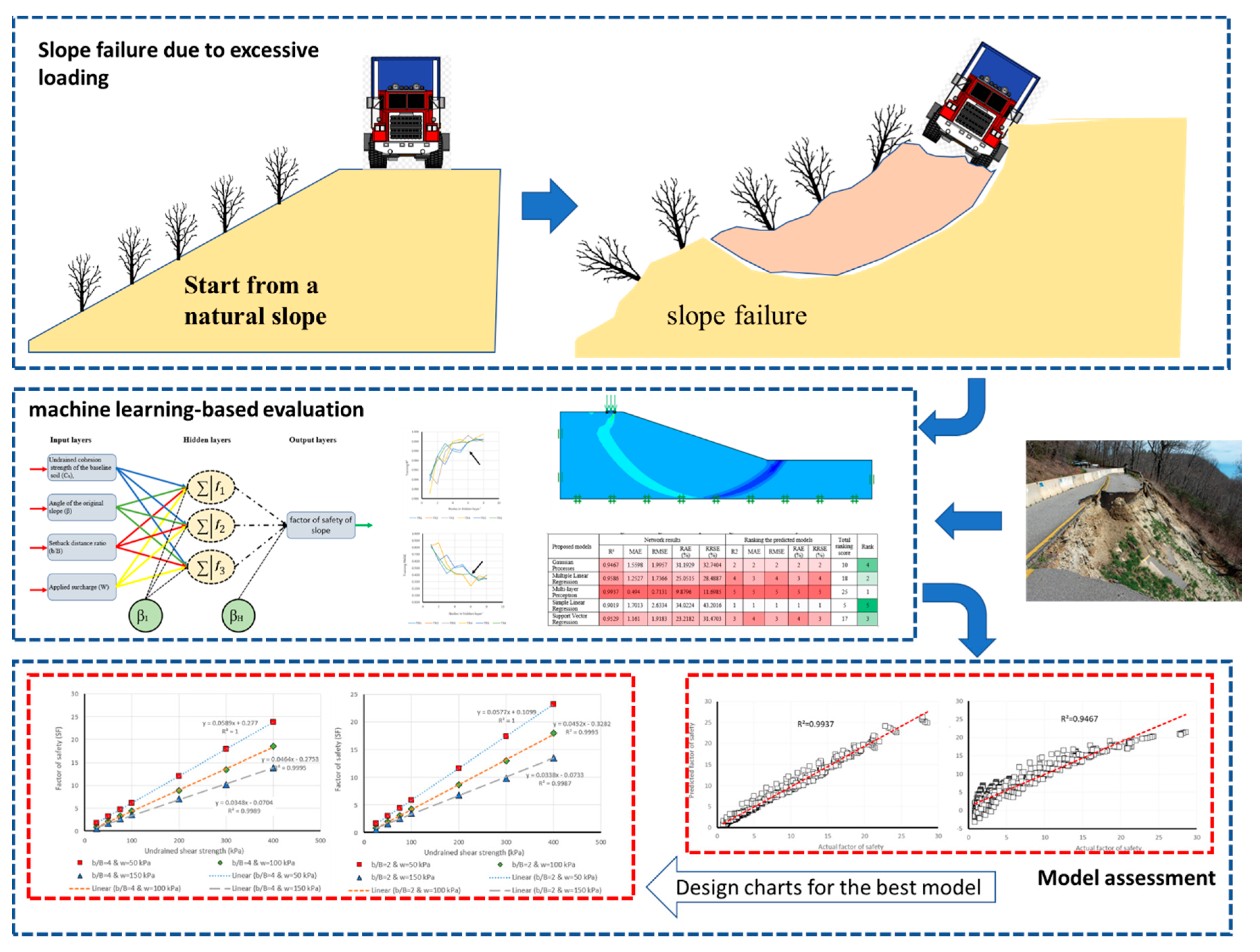
:In this study, we employed various machine learning-based techniques in predicting factor of safety against slope failures. Different regression methods namely, multi-layer perceptron (MLP), Gaussian process regression (GPR), multiple linear regression (MLR), simple linear regression (SLR), support vector regression (SVR) were used. Traditional methods of slope analysis (e.g., first established in the first half of the twentieth century) used widely as engineering design tools. Offering more progressive design tools, such as machine learning-based predictive algorithms, they draw the attention of many researchers. The main objective of the current study is to evaluate and optimize various machine learning-based and multilinear regression models predicting the safety factor. To prepare training and testing datasets for the predictive models, 630 finite limit equilibrium analysis modelling (i.e., a database including 504 training datasets and 126 testing datasets) were employed on a single-layered cohesive soil layer. The estimated results for the presented database from GPR, MLR, MLP, SLR, and SVR were assessed by various methods. Firstly, the efficiency of applied models was calculated employing various statistical indices. As a result, obtained total scores 20, 35, 50, 10, and 35, respectively for GPR, MLR, MLP, SLR, and SVR, revealed that the MLP outperformed other machine learning-based models. In addition, SVR and MLR presented an almost equal accuracy in estimation, for both training and testing phases. Note that, an acceptable degree of efficiency was obtained for GPR and SLR models. However, GPR showed more precision. Following this, the equation of applied MLP and MLR models (i.e., in their optimal condition) was derived, due to the reliability of their results, to be used in similar slope stability problems.
1. Introduction
The stability of natural slopes has a significant impact on civil engineering infrastructures (e.g., earth dams, and transmission roads) that rest near them. This issue can be considered for different types of slopes, such as artificial and natural slopes. Hence, having a good approximation from the stability of such slopes is a vital task. Note that the purposed approaches must have enough reliability, as well as the least computational time for engineering utilization [1,2]. Up to now, many scholars have developed different techniques for slope stability assessment, like limit equilibrium methods (LEM) and numerical solutions [3,4]. In a general view, there are some defects for the mentioned methods (difficultness to determine the rational mechanical parameters, for instance) that make them cumbersome to implement [5]. Another important disadvantage of traditional slope stability solution is related to the time and cost constraints for implementing such models. So, many researchers have focused on generating the design charts to be used toward slope analysis [6]. This is while the appearance of the computational solutions has made most diagrammatic methods antiquated [7,8]. Zhou, et al. [9] proposed novel prediction technique that employ the gradient boosting machine (GBM) technique to analyze the stability of slopes. It is found that the GBM proposed model has high reliability for the estimating stability of slopes. Over the last decade, the application of soft computing predictive tools has increased, due to their capability of establishing nonlinear equations between a set of input-output data. In this field, various types of artificial neural network (ANN) [10] and support vector machines (SVM) [11] have been successfully employed for simulating geotechnical problems. The notable advantage of ANNs is that they can perform by any defined number of neurons, as in their hidden layer [12,13,14,15]. In addition, no former knowledge of data processing is needed. On the other hand, overfitting of the network as well as being trapped in local minima can be mentioned as essential drawbacks of ANNs. A regression-based method such as Gaussian processes regression (GPR) and simple linear regression (SLR) have attracted far attention in many research fields such as traffic forecasting [16], tourism demand approximation [17] and signal processing [18]. Similarly, plenty of complex geotechnical problems have been modelled with this approach [19,20,21]. Zhang et al. [22] developed a GPR-based solution for the slope stability problem. According to their results, this model is useful and simply-used, which can act as the superior approach compared to the ANN and SVM methods published in prior studies. In another research, Jagan et al., [7] developed four common models namely, GPR, adaptive neuro-fuzzy inference system (ANFIS), relevance vector machine (RVM), and extreme learning machine (ELM) to appraise the stability number of layered slopes. Their results revealed the advantage of the ELM in comparison with other developed machine learning-based tools. In a work by Chakraborty and Goswami [23,24] for estimating the factor of safety of a slope, the results obtained by the ANN and MLR models were compared to a finite element method (FEM). They found that both applied tools (i.e., ANN and MLR) are accurate enough to be used in this field. Also, a higher degree of precision was acquired for ANN compared to MLR. Mosavi, et al. [25] stated the machine learning-based techniques as cost-effective solutions. They have introduced various machine learning-based solutions in flood prediction in order to give insight into the most appropriate models.
However, few scholars have attempted to present comparative research for slope failure assessment [26]; no prior study was found to evaluate the effectiveness of the models mentioned above, simultaneously. Therefore, this study aims to assess and compare the efficiency of various machine learning-based methods for slope stability modelling. Furthermore, due to the previously stated constraints of traditional methods, another novelty of this work can be highlighted by presenting an operational formula for appraising the FS of similar slopes. In this sense, we developed five conventional soft computing approaches including Gaussian process regression (GPR), multi-layer perceptron (MLP), simple linear regression (SLR), support vector regression (SVM), and multiple linear regression (MLR), to calculate the safety factor of a single-layered slope (i.e., modelled based on cohesive materials). To do so, four influential factors affecting the risk of slope failure were considered for this study. Undrained shear strength (Cu), slope angle (β), setback distance ratio (b/B), and applied surcharge on the shallow foundation installed over the slope (w) opted. To prepare the required dataset, respecting to the mentioned variables, 630 different analyzed stages of the purposed soil slope were performed in the Optum G2 software and the safety factor obtained for each corresponding input conditions were taken to be the output. In the following, 80% of the whole dataset was specified for training the GPR, MLR, MLP, SLR, and SVR models. The remained 20% was used to assess the performance of models. Note that different statistical indices were employed to calculate the error and correlation between the real and predicted safety factor.
2. Machine Learning and Multilinear Regression Algorithms
2.1. Gaussian Processes Regression (GPR)
Gaussian processes regression (GPR) is one of the appropriate, and newly-proposed methods that have been employed for may machine learning examples [27]. The probabilistic solution that is developed by GPR model leads to discerning generic regression problems with kernels. The training process of the applied regressor can be classified within a Bayesian framing, and it has been supposed that the model relations follow a Gaussian distribution to encode the former information about the output function [28]. The Gaussian process is specified by a series of variables that there is a joint Gaussian allocation for each one of them [29]. The following equation describes the overall structure of the Gaussian process:
where w(x) designates, the Gaussian process mean function and indicates the kernel function.
Consider a learning dataset that is built by N pairs in the form of where in this dataset, x is defined as an N-dimensional input vector where corresponding target is taken as y. The GPR model helps the below formulation to discover the relationship between the given inputs and targets taking xj as a test sample [29].
where wj defines mean value representing the most compatible predicted outputs for the test input vector (xj). Also, K(X, X), kj, , and y stand for the covariance matrix, the kernel distance between training and testing data, the noise variance, and training observation, respectively. As well as this, the produced variance by Equation (3) (), represents a confidence measure related to the obtained results. Note that, this variance is adversely proportional to the confidence associated with the wj [30]. The above formulas can be gathered in the form of a linear combination of the s kernel function and the mean estimation for (xj) can be expressed as follows:
2.2. Multiple Linear Regression (MLR)
The focal goal of multiple linear regression (MLR) model is to establish a linear equation to the data samples to reveal the relationship between two or more independent (explanatory) variables and a dependent (response) variable. The overall structure of the MLR formula is shown by Equation (5) [31]:
In the above formula, y and x represent the dependent and independent variables, respectively. The terms α0, α1, … αs are indicative of MLR unknown parameters. Also, the normally distributed random variable is shown by ε in MLR generic formula.
The main task of MLR is to approximate the unknown terms (i.e., α0, α1, … αs) of Equation (5). After applying the least-square technique, the practical form of the statistical regression method is given by [31]:
where a0, a1, … as are the approximated regression coefficients of α0, α1, … αs, respectively. Also, term e describes the approximated error for the sample. Assuming the term e as the difference between the actual and predicted y, the estimate of y is as follows:
2.3. Multi-Layer Perceptron (MLP)
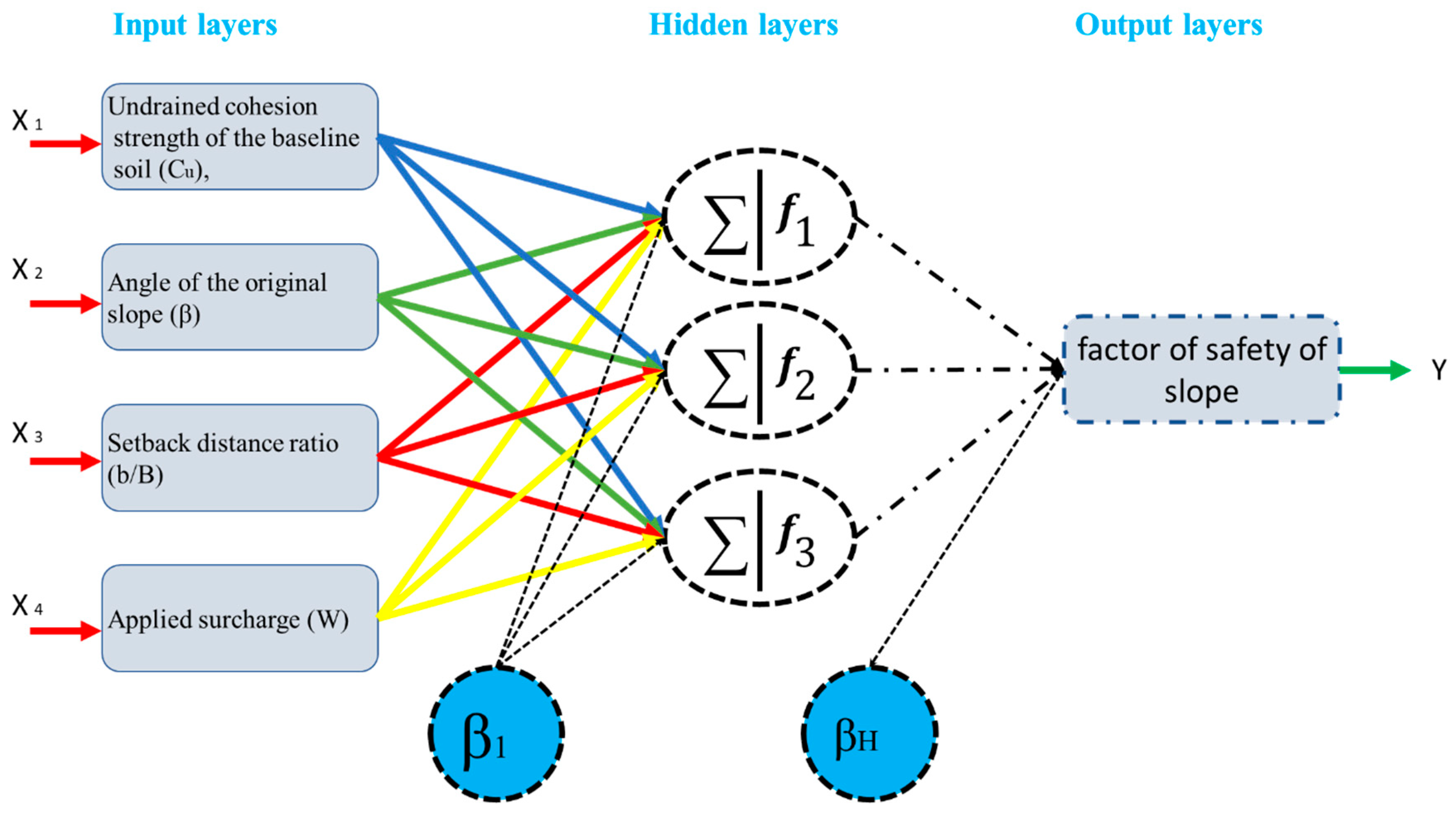
Artificial neural networks (ANNs) are capable of predictive tools that were introduced by [32], mimicking the biological neural network. multi-layer perceptron (MLP) is a common type of ANNs that have shown a satisfying performance dealing with many engineering simulations [33,34,35,36,37]. This is due to their ability in generating non-linear equations between the set of inputs and outputs [38,39]. Figure 1 denotes the general structure of MLP. A simple MLP neural network is constructed from three layers containing computational nodes (mostly known as neurons).
The initial data are received by the nodes in the input layer. In the following, hidden neurons (i.e., the neurons in the hidden layer) attempt to discover the relationship between the inputs and the corresponding targets, through assigning and adjusting the MLP weights and biases. After that, the output is produced by the neurons performing in the last layer (i.e., output layer). More particularly, assume the S and W, respectively as the input and weight vectors. Then the performance of each neuron is formulated as follows:
where j is the number of neurons, and b indicates the bias. Also, F(x) stands for the activation function (AF). Note that, a feed-forward back-propagation (FFBP) method is considered for this study, which aims to minimize the error performance by adjusting the MLP parameters (i.e., weights and biases). The FFBP method is well-discussed in other works [40].
2.4. Simple Linear Regression (SLR)
The main objective of simple linear regression (SLR) is to investigate the effect of a predictor variable on a specific output. As the name demonstrates, the relationship between input-target samples is described by a linear dependency in this model. The formulation of a simple linear regression is generically presentable in the form of Equation (10):
where x and y are the independent and dependent variables, respectively, the terms α and β indicate the structural parameters (intercept on the y-axis and the slope of the regression line, respectively). In addition, the random error is defined by κ, which is supposed to be uncorrelated with a mean of zero and fixed variance. Furthermore, in order to obtain a higher competency in prediction, the analyses are often associated with the assumption of the normal distribution of errors [41]. Note that, transformation process may be carried out to achieve desired normality of data [42].
Considering a population of samples like the SLR method applies the ordinary least square (OSL) method to approximate the structural parameters (i.e., α and β). Having a normal distribution is not essential, but it helps the regression model to have more accuracy [41]. With this in mind, the developed regression model aims to find its parameters such that the lowest value of the sum of squared error (i.e., the difference between the actual and estimated data) is obtained [43]. Finally, after determining the proper values of α (intercept) and β (slope regression parameter), the fitted output (yi) can be calculated at any given x value (xi).
2.5. Support Vector Regression (SVR)
Support vector machine (SVM) is one of the widely-employed machine learning algorithms which aimed to detect the decision boundary in order to separate different classes. Due to their outstanding presentation to deal with examples of the non-separable and high-dimensional data sets, SVMs have been effectively applied as a reliable solution for many classification problems [44]. Theoretically, the training process of SVM techniques is evinced by the statistical theories [45]. Therefore, the mechanism of SVMs is mainly based on the transformation from non-linear to future linear spaces [46]. A well-known type of SVMs is support vector regression (SVR). As the name implies, the main application of SVRs is to solve the complex regression problems. During SVR learning, it is assumed that there is a unique relationship between each set of input-target pairs. Grouping and classifying the relation of these predictors will conduce to produce the system outputs (e.g., slope safety factor in this study) [47]. Unlike many predictive models that try to minimize the calculated error (i.e., the difference between the target and system outputs), SVR aims to improve its performance by optimizing and altering the generalization bounds for a regression. In this subject, a predetermined error value can be ignored by a ε-insensitive loss function (LF) [48]. If we assume a training dataset that is formed by N pairs of samples, represented by the SVR model containing the mentioned LF (i.e., ε-SVR) attempts to find the optimum hyperplane that it has the minimum distance from all sample points. More specifically, ε-SVR seeks a function g(x) that has the highest ε deviation from the target data (i.e., yi) [49]. As explained in previous sentences, the linear regression is implemented in high dimensional feature space using ε-LF. Moreover, the lower value for , the less complex model [50]. As for the non-linear problems, the input data are transformed into high-dimensional space by means of a kernel mapping function indicated by γ(xi). After that, a linear approach is applied to data in the future space by a convex optimization problem [45,51].
where the terms w and C are indicative of weight vector (i.e., in the future space) and penalty parameter, respectively. This must be noted that the trade-off between the performance error and the complexity of the model is ascertained by C constant. Also, b defines the bias and the parameters ϕi and ϕi* stand for the slack variables measuring the deviation of training data outside ε-LF zone. The precision factor is also shown by ε in the above formula [52]. In other words, only samples with a deviation value more than ε will be considered for error function [51]. Eventually, to calculate the SVR results, a linear combination is established associated with introducing Lagrange multiplier of ρi and ρi*:
3. Data Collection
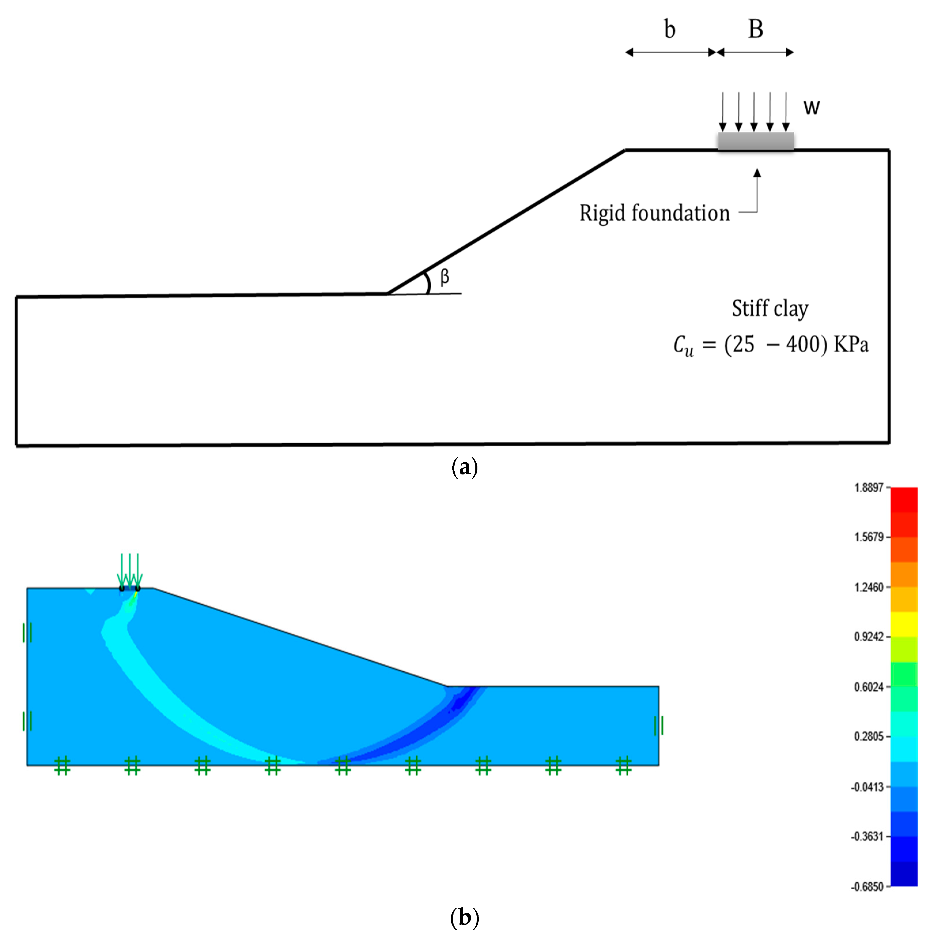
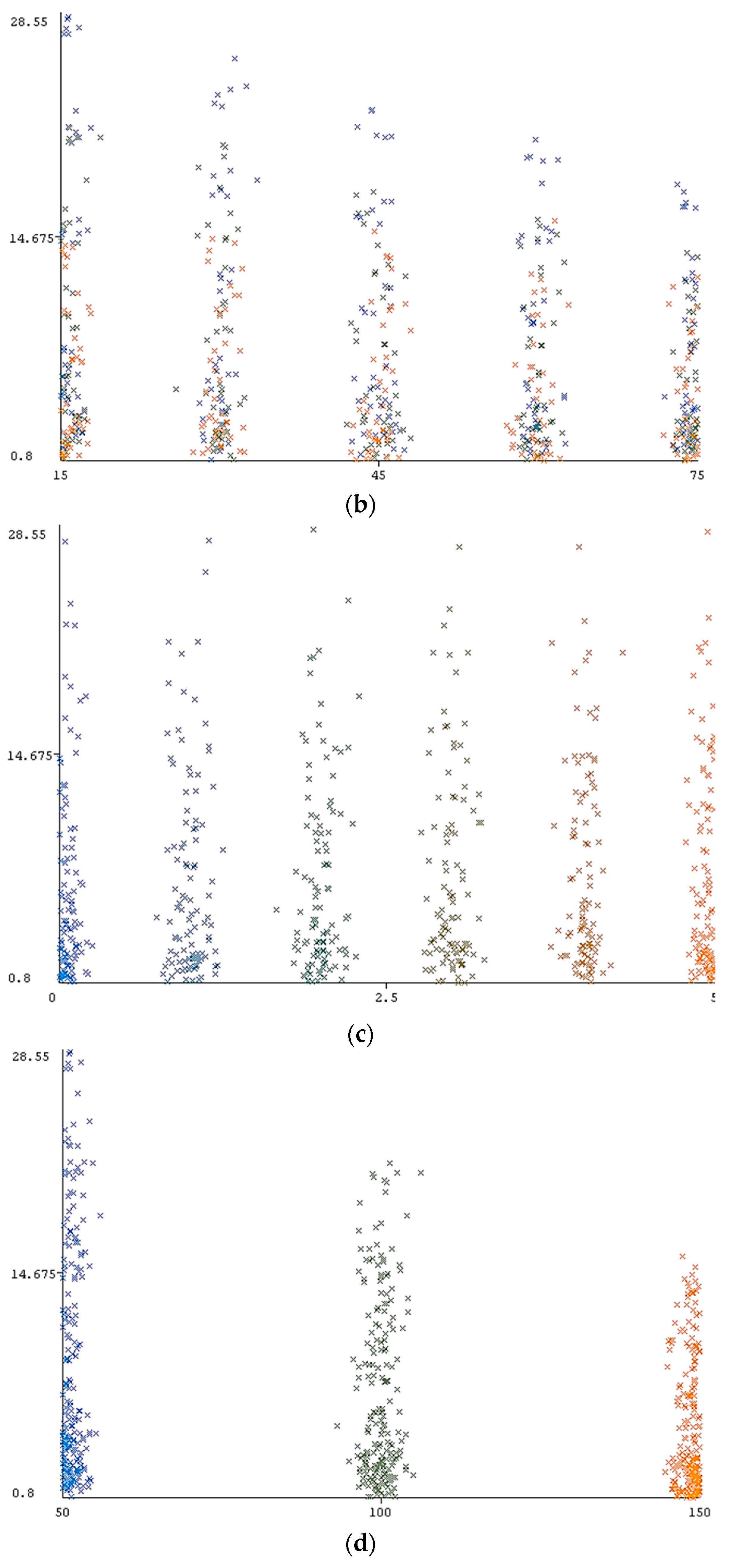
The main motivation of the present research is to evaluate the applicability of various machine learning-based tools to the subject of slope stability assessment. Several regression methods namely, Gaussian process regression (GPR), multiple linear regression (MLR), multi-layer perceptron (MLP), simple linear regression (SLR), support vector regression (SVR) were implemented in WEKA software. A purely cohesive soil layer constructs the slope geometry that only has undrained cohesive strength (see Figure 2a). In order to estimate the safety factor of the purposed slope, four effective parameters including undrained shear strength (Cu), slope angle (β), setback distance ratio (b/B), and applied surcharge on the footing installed over the slope (w) opted in this work. To create the required dataset, Optum G2 computer software [53,54] was used, which follows a comprehensive finite element method (FEM) (see Figure 2b). Considering the mentioned influential variables, 630 different stages were analyzed, and the safety factor was derived as the output. During the model development, the elastic parameter of Young’s modulus (E) was supposed to be different for each value of Cu. In this regard, E was 1000, 2000, 3500, 5000, 9000, 15,000 and 30,000 kPa for respective Cu values of 25, 50, 75, 100, 200, 300 and 400 kPa. As well as this, the numbers 0.35, 18 KN/m3, and 0° were allocated to the mechanical parameters Poisson’s ratio, soil unit weight, and internal friction angle, respectively. For more details, the relationship between the computed F safety factor S and its conditioning factors (i.e., Cu, β, b/B, and w) is demonstrated in Figure 3a–d, showing the safety factor featured on the vertical axis versus the respective parameters of Cu, β, b/B, and w, on the horizontal axis. In all diagrams, the slope safety factor varies from 0.8 to 28.55. As is expected, a proportional distribution can be found for the Cu (25, 50, 75, 100, 200, 300, and 400 kPa) and obtained safety factor (see Figure 3a). Adversely, in a general view, when the values of β (15°, 30°, 45°, 60°, and 75°) and w (50, 100, and 150 KN/m2) are increased, more instability is observed (see Figure 3b,d). In addition, according to Figure 3c, different values of safety factor have been reported as the purposed foundation takes more distance from the edge of slope (b/B is determined by 0, 1, 2, 3, 4, and 5 values).
The produced dataset was randomly divided into training and testing phases. The training stage consisted of 504 samples (i.e., 80% of the whole dataset) specified to the primary learning process. The remaining 126 samples (i.e., 20% of the whole dataset) were used to evaluate the performance of GPR, MLR, MLP, SLR, and SVR methods (Figure 3). Figure 4 illustrated the scheme of development of the database and selected methodology.
4. Results and Discussion
The main objective of the present study is to investigate the feasibility of five common machine learning-based methods, namely, GPR, MLR, MLP, SLR, and SVR for slope stability assessment. This work carried out by means of the factor of safety estimation. To this purpose, four conditioning parameters affecting the stability of a single-layered cohesive slope opted to be Cu, β, b/B, and w. Referring to the various possible quantities for these parameters, 360 different stages were defined and analyzed in Optum G2 finite element software, and the safety factor was taken as the output. The required data set was gathered for training the purposed models in WEKA software. The results of this part have been reported by various validation indices such as relative absolute error (RAE in%), coefficient of determination (R2), root mean square error (RMSE), mean absolute error (MAE), and root relative squared error (RRSE in%). A colour intensity rating is also generated to display a hued ranking of the implemented models. The quality of results is adversely proportional to the intensity of the colour (green) in the last column of each table. In contrast, more intense colour (red) indicates a more proper performance for all other columns. This is noteworthy that these criteria have been widely used in earlier studies (e.g., Moayedi and Hayati [37], Vakili, et al. [55] and Moayedi and Armaghani [56]). Equations (14)–(18) presented the formulation of R2, MAE, RMSE, RAE, RRSE, respectively.
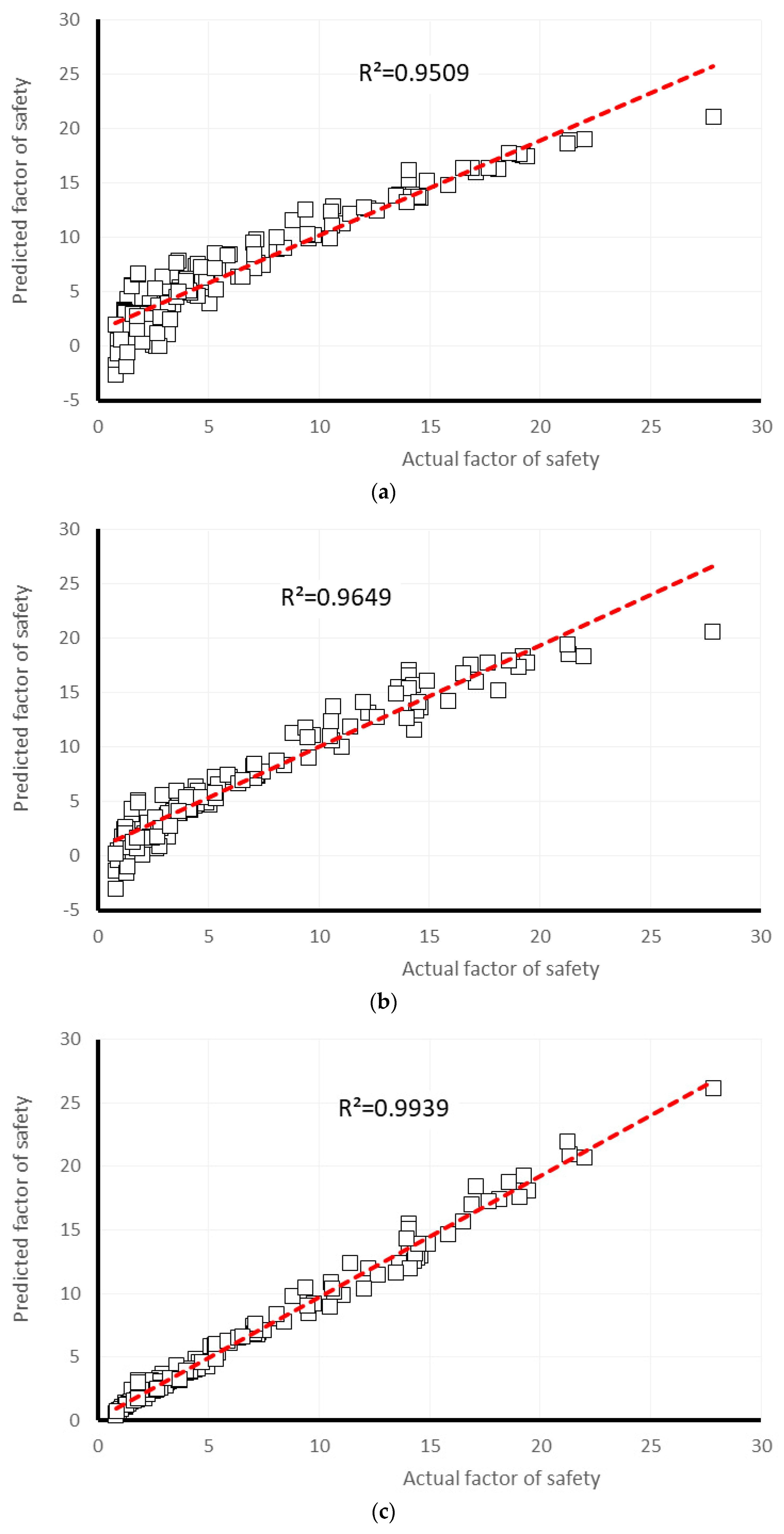
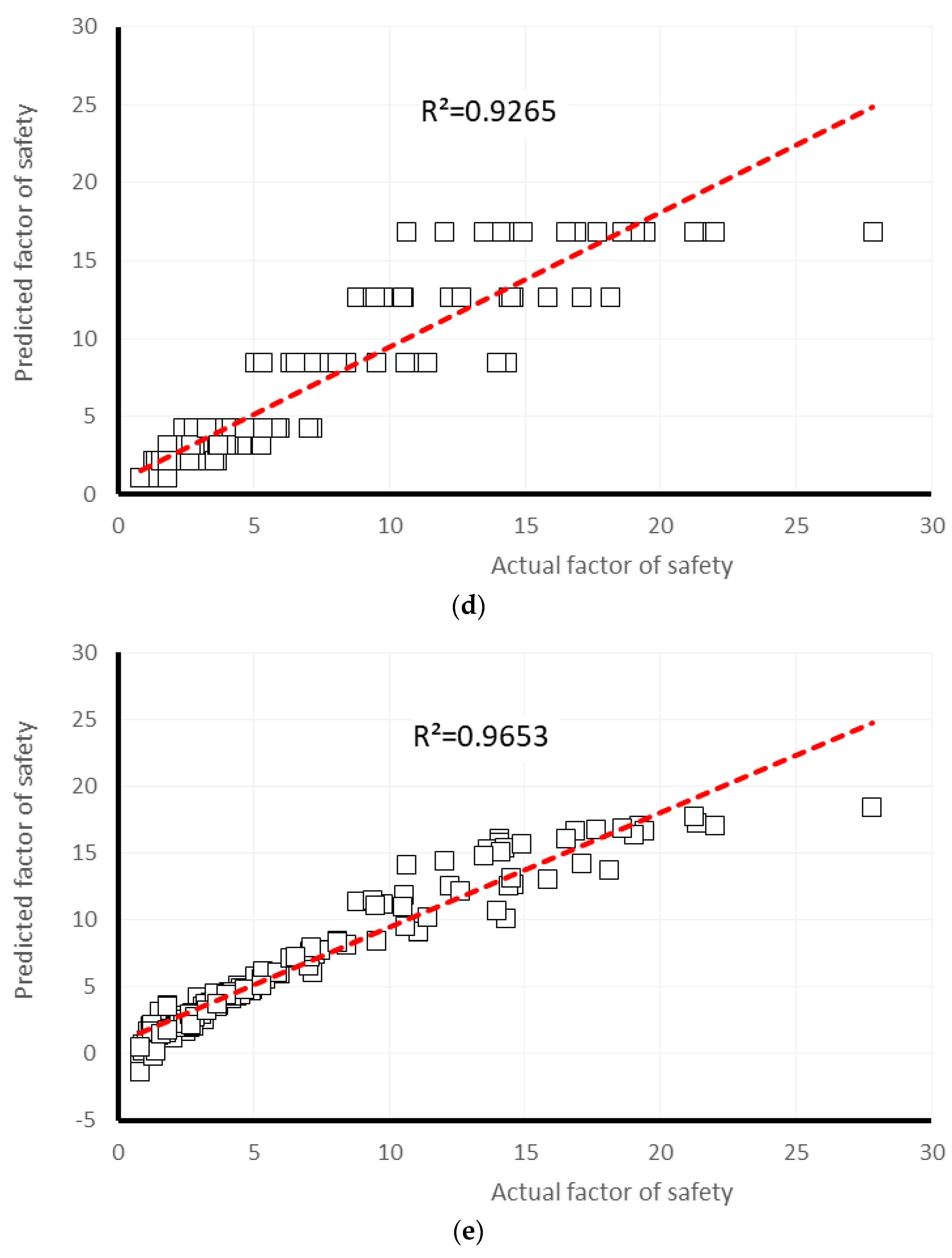
where in all the above relationships Yi observed and Yi predicted indicates the actual measurement and estimated slope safety factor, respectively. The term S is the defined of the number of data; is the mean of the real values of safety factor. The obtained values of R2, MAE, RMSE, RAE, RRSE for safety factor estimation are tabulated in Table 1 and Table 2, respectively, for the training and testing phases. In a glance, MLP is qualified as the first ranking model for both tables. For the training results, based on the R2 (0.9467, 0.9586, 0.9937, 0.9019, and 0.9529), RMSE (1.9957, 1.7366, 0.7131, 2.6334, and 1.9183), and RRSE (32.7404%, 28.4887%, 11.6985%, 43.2016%, and 31.4703%), respectively for GPR, MLR, MLP, SLR, and SVR models, the MLP outputs have shown the best accommodation with the actual values of safety factor. After that, SVR and MLR have also presented a high level of accuracy. In addition, GP (4th ranking) and SLR (5th ranking) have shown an acceptable rate of accuracy concerning the calculated MAE (1.5598 and 1.7013, respectively) values. The sole distinction for the final results (i.e., last column) in Table 1 and Table 2 refers to the ranking gained by MLR and SVR predictive models. As is clear, SVR as the second-accurate model has shown more sensitivity for the testing stage compared to the MLR. In addition, the obtained results for the testing dataset confirms the higher capability of MLP. Considering the respective values of R2 (0.9509, 0.9649, 0.9939, 0.9265, and 0.9653), MAE (1.5291, 1.1949, 0.5155, 1.5387, and 1.0364), and RAE (30.9081%, 24.1272%, 10.4047%, 31.0892%, and 20.9366%), it can be concluded that SVR is the second-precise model, and MLR has outperformed GP and SLR.
Table 3 demonstrates the total efficiency ranking of developed models (i.e., the summation of R2, MAE, RMSE, RAE, RRSE single ranking for training and testing dataset). Based on the obtained total scores of 20, 35, 50, 10, and 35 (respectively for GPR, MLR, MLP, SLR, and SVR), the superiority of MLP can be deduced (i.e., the most significant total rank). The multiple linear regression and support vector regression methods have commonly been labelled as the second-accurate models. After these, GPR and SLR have shown a good quality of safety factor estimation with respective total scores of 20 and 10. The remarkable point about Table 3 is that an equal individual score for all indices has featured for MLP, GPR, and SLR predictive model. The MLP and SLR, for instance, had the highest (5) and lowest (1) level of accuracy, based on the R2, MAE, RMSE, RAE, and RRSE indices simultaneously.
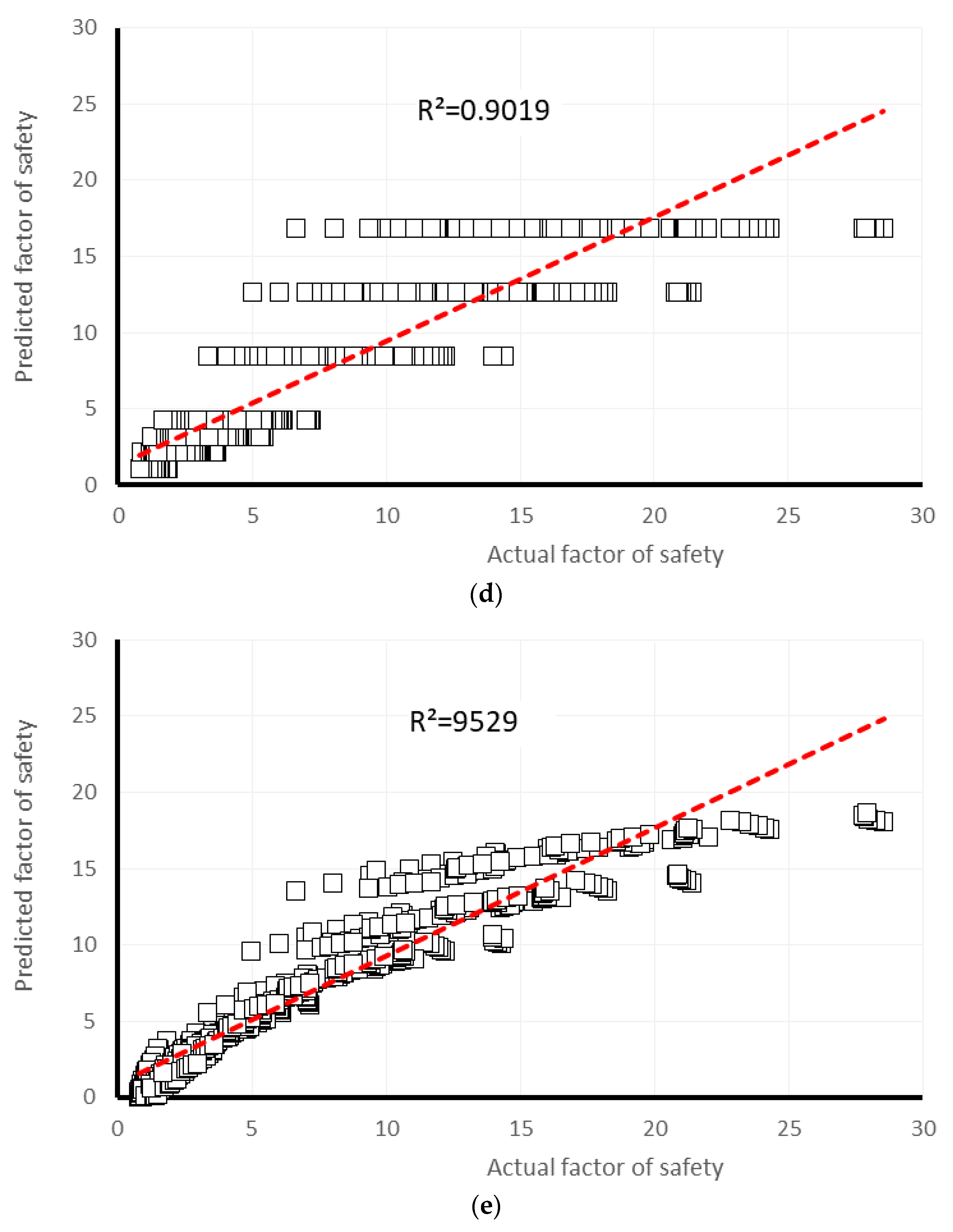
Many studies have revealed that the machine learning-based techniques are reliable methods for approximating the engineering complex solutions [57,58,59,60,61]. Many of these learning systems are available in Waikato Environment for Knowledge Analysis (Weka). Furthermore, the pictorial correlation between the measured (on the horizontal axis) and predicted (on the vertical axis) safety factor is shown in Figure 5a–e, for training dataset, and Figure 5a–e, for testing dataset, respectively for GPR, MLR, MLP, SLR, and SVR models. Comparing the observed regression in Figure 5 and Figure 6, the trend line has been drawn for MLP and MLR results, have the most inclining to the line y = x (i.e., R2 = 1).
The graphical view of the computed error (the difference between the observed and predicted slope safety factor) for all employed models is depicted in Figure 7. As is obvious in this chart, the less distance from the y = 0 axis (i.e., the lowest error), results in higher accuracy. In this subject, the MLP and SVR models have presented the most reliable prediction, due to the higher aggregation of their results around the y = 0 axis, particularly for the first 350 data. In contrast, the maximum observed error is obtained for the SLR estimation, which reaches more than ten units, for both negative and positive error.
Referring to the results, it can be concluded that MLP (R2 = 0.9937 and 0.9939, and RMSE = 0.7131 and 0.7039, respectively for training and testing phases) and MLR (R2 = 0.9586 and 0.9649, and RMSE = 1.7366 and 1.5891, respectively for training and testing phases) predictive models are eligible enough to provide an appropriate estimation for safety factor. In addition, the obtained values of RRSE for training (11.6985% and 28.4887%, respectively for MLP and MLR) and testing (11.8116% and 26.4613%, respectively for MLP and MLR) datasets prove a high level of accuracy for these techniques. With this in mind, in this part of the current study, it was aimed to extract the equation of developed MLR and MLP models to be used in stability assessment of similar slopes. The MLR attempts to fit a linear relationship to data. The formula derived from the MLR and MLP models is presented in Equations (19) and (20), respectively.
where terms Y1 and Y2 are calculated from the below equations:
FSMLP = (−1.12353500504828 × Y1) − (2.38866337313669 × Y2) + 1.77734928298793
5. Design Charts
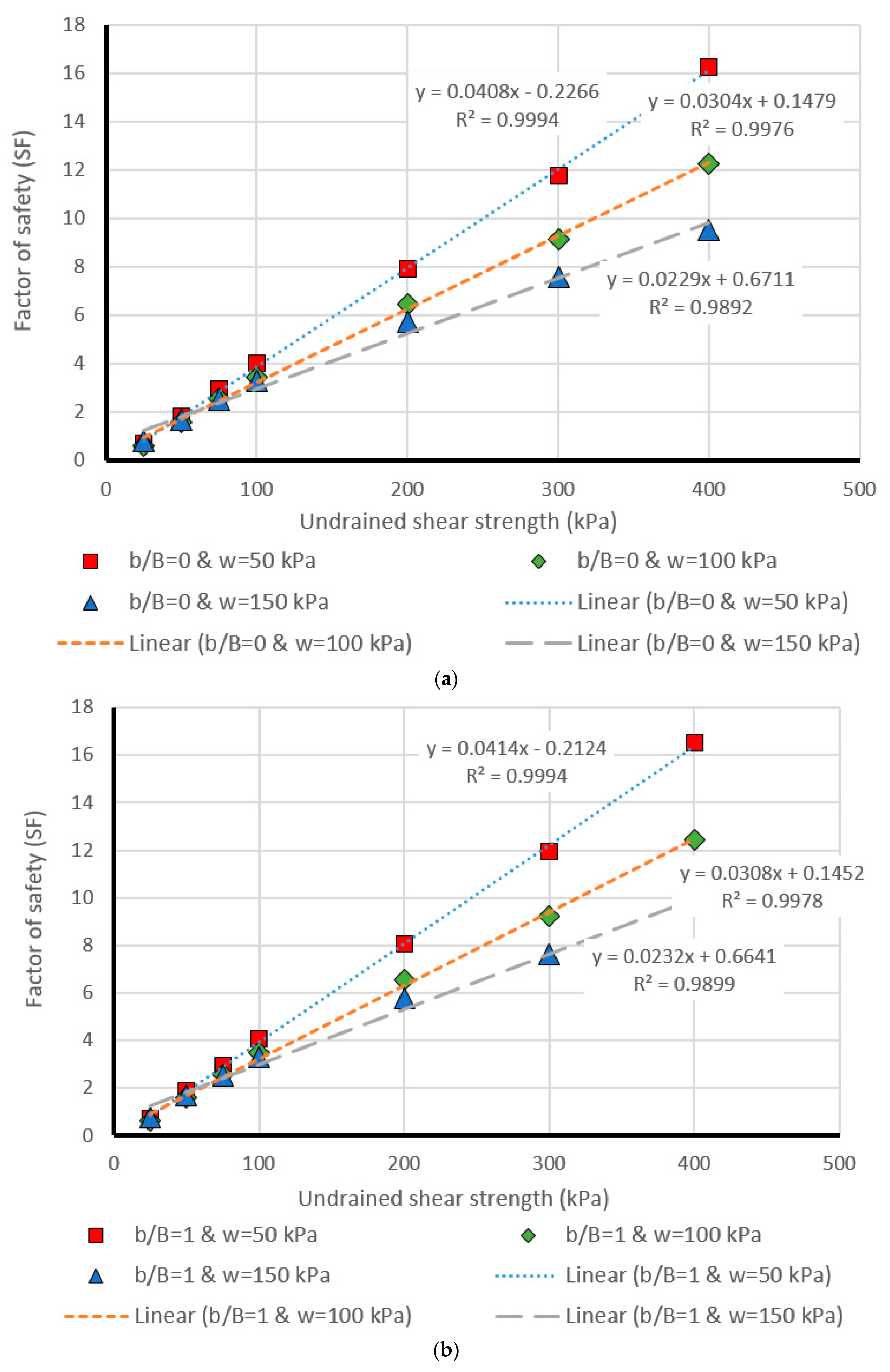
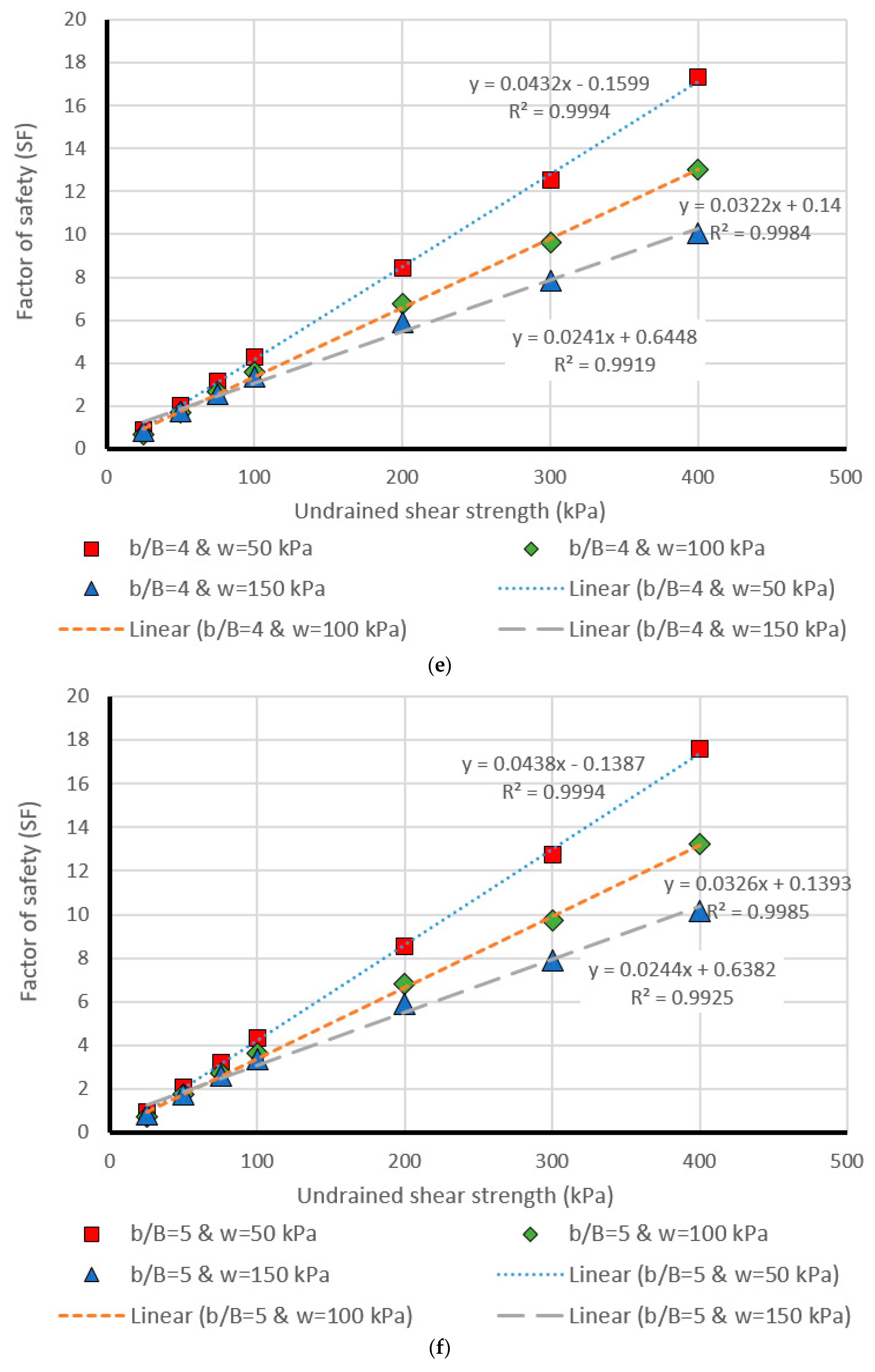
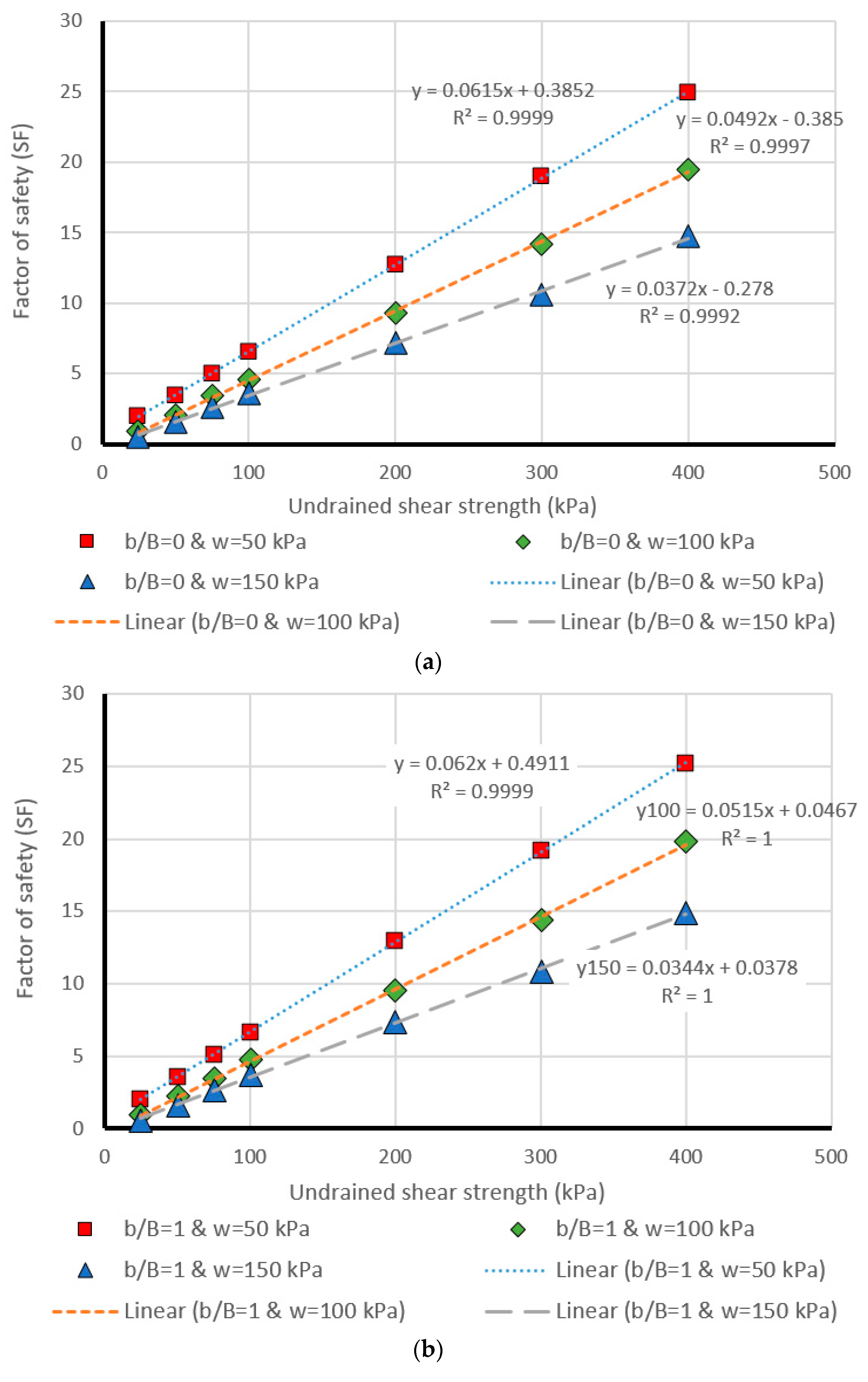
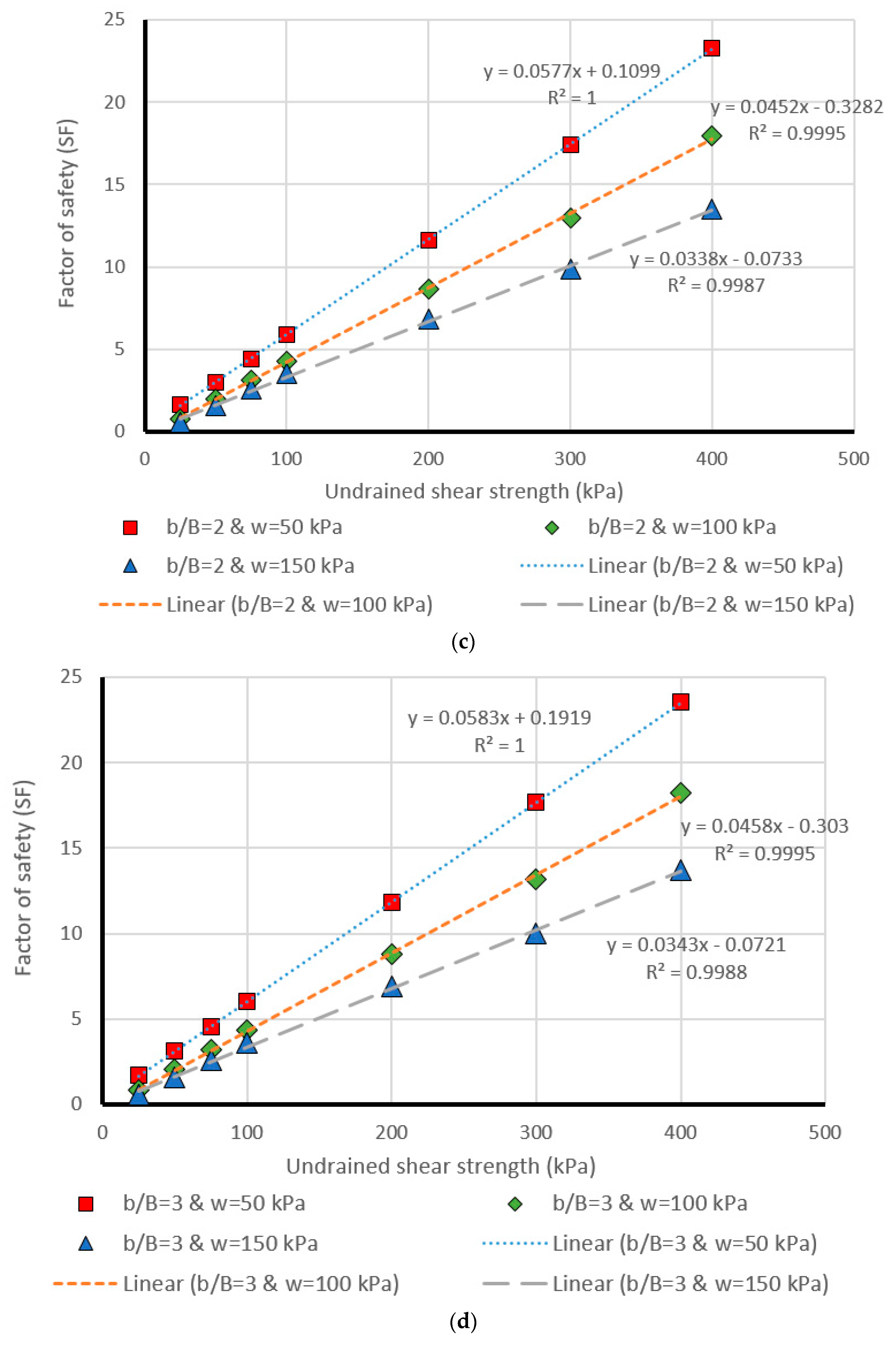
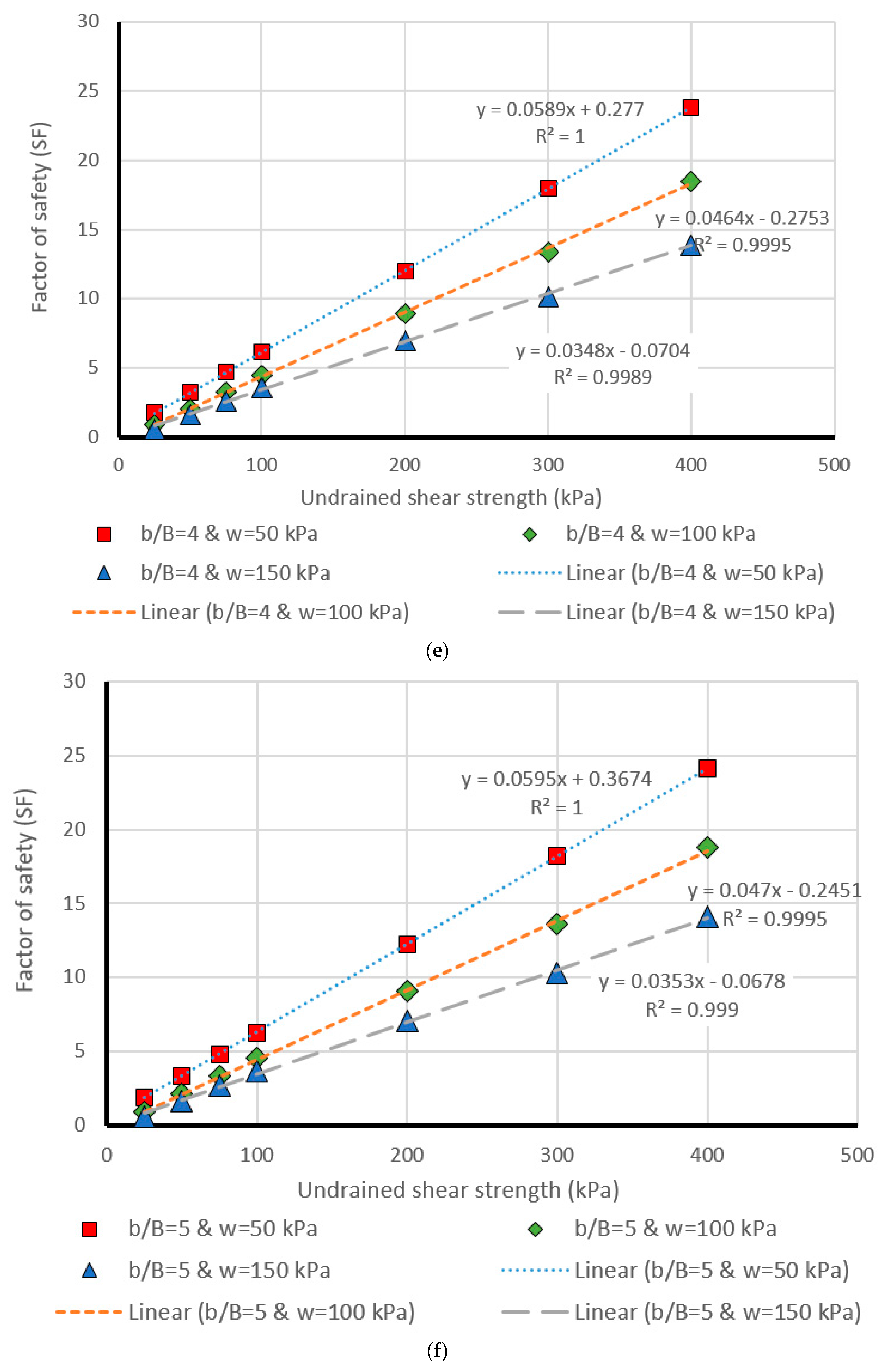
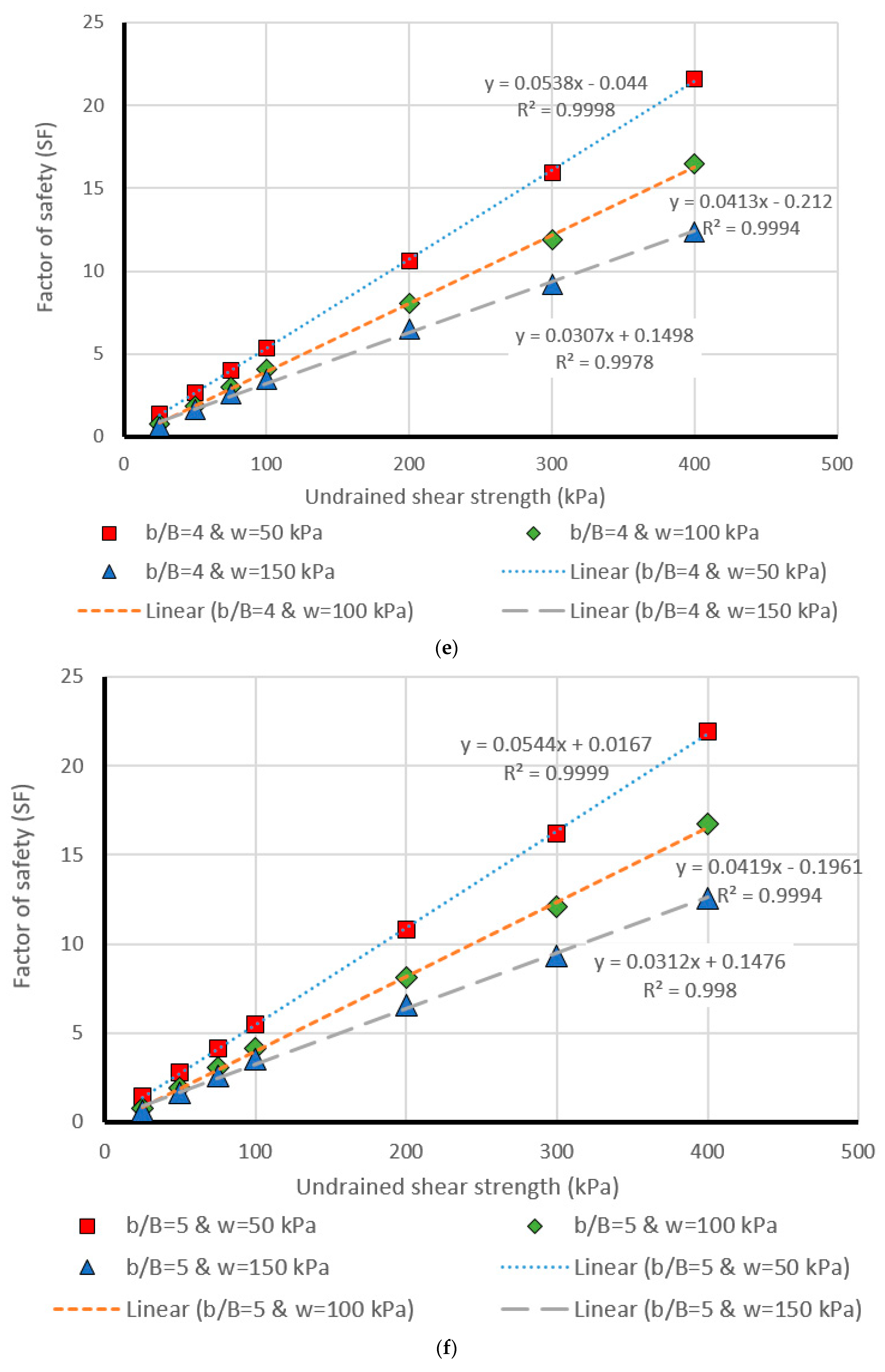
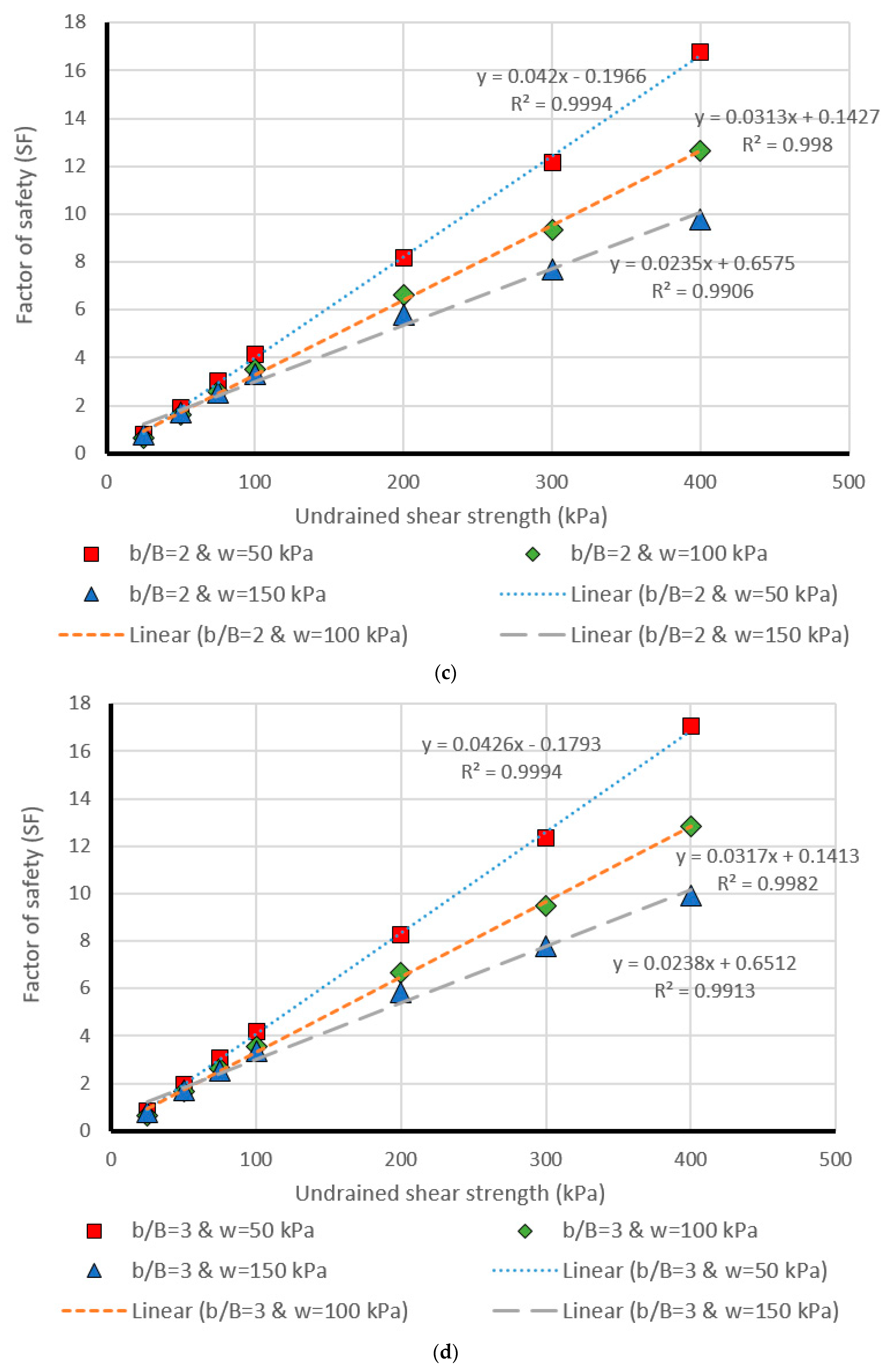
The last part of this paper deals with presenting a more detailed evaluation of the results obtained by the most successful model, i.e., MLP. This was carried out through comparing the estimated and real values of safety factor within design chart figures, generated for different values of effective factors (i.e., Cu, β, b/B, and w). Moreover, having a more detailed presentation from the results of MLP (i.e., the most successful method), in the last part of this research, it was aimed to compare the actual and MLP estimation of safety factor in several separate stages. To this purpose, Figure 8, Figure 9, Figure 10, Figure 11 and Figure 12 were drawn (for different values of β = 15°, β = 30°, β = 45°, β = 60°, and β = 75°) showing the safety factor (on the vertical axis) against the undrained shear strengths (Cu) (on the horizontal axis). Note that these figures are provided as an appendix. Each single chart illustrates the comparison between the real (i.e., linear) and predicted (i.e., points) values of safety factors, for different values of b/B ratio ((a), (b), (c), (d), (e), and (f), respectively for b/B = 0, b/B = 1, b/B = 2, b/B = 3, b/B = 4, and b/B = 5). Note that, in all charts, the data have been divided into three parts concerning the w (applied surcharge on the rigid foundation) values, which were 50, 100, and 150 kPa. Based on the coefficient of determination (i.e., R2) computed for each case, the effectiveness of estimation carried out in this study can be deduced.
6. Conclusions
Due to the inevitability and undeniable impacts of the slope failure phenomena on many geotechnical projects, the main motivation of the current research was to evaluate the applicability of various machine learning and regression-based models in predicting the factor of safety of slope. In this purpose, GPR, MLR, MLP, SLR, and SVR models were developed. A single-layered cohesive slope was assumed. Four influential parameters affecting the stability of the slope, namely Cu, β, b/B, and w were considered in this study. To create the eligible dataset, referring to possible values that can be received by mentioned effective parameters, 630 different stages were defined and analyzed in Optum G2 software. The factor of safety was picked as the output of this operation. In the next step, the acquired dataset was divided into training (80% of the entire dataset) and validation (20% of the entire dataset) phases to train and validate the efficiency of GPR, MLR, MLP, SLR, and SVR approaches. The implementation of models was carried out in WEKA software, which is a prominent tool for machine learning and classification applications. For the training phase, the R2 (0.9467, 0.9586, 0.9937, 0.9019, and 0.9529), MAE (1.5598, 1.2527, 0.4940, 1.7013, and 1.161), RMSE (1.9957, 1.7366, 0.7131, 2.6334, and 1.9183), RAE (31.1929%, 25.0515%, 9.8796%, 34.0224%, and 23.2182%), and RRSE (32.7404%, 28.4887%, 11.6985%, 43.2016%, and 31.4703%), were obtained, respectively for GPR, MLR, MLP, SLR, and SVR. Similarly, for the testing phase, we acquired R2 (0.9509, 0.9649, 0.9939, 0.9265, and 0.9653), MAE (1.5291, 1.1949, 0.5155, 1.5387, and 1.0364), RMSE (1.9447, 1.5891, 0.7039, 2.2618, and 1.6362), RAE (30.9081%, 24.1272%, 10.4047%, 31.0892%, and 20.9366%), and RRSE (32.3841%, 26.4613%, 11.8116%, 37.6639%, and 27.2470%), respectively for GPR, MLR, MLP, SLR, and SVR. Referring to the indices mentioned above, the advantage of MLP is deduced, compared to the other applied machine learning methods. In addition, it can be seen that there is a slight difference between the performance of MLR and SVR predictive models, and GPR outperforms SLR. In the next section, the equation of implemented MLP and MLR (i.e., for their optimal condition) was derived to be used in similar slope stability problems. In addition, due to the highest rate of success for MLP prediction, in the last part, the outputs produced by this model were more particularly compared to the actual values of safety factor within design charts generated for different values of Cu, β, b/B, and w.
Author Contributions
H.M. and D.T.B. performed experiments and field data collection; H.M. wrote the manuscript, discussion and analyzed the data. M.G. and A.J., and L.K.F. edited, restructured, and professionally optimized the manuscript.
Funding
This research received no external funding.
Acknowledgments
This work was financially supported by Ton Duc Thang University and University of South-Eastern Norway.
Conflicts of Interest
The authors declare no conflicts of interest.
References
- Qi, C.; Tang, X. Slope stability prediction using integrated metaheuristic and machine learning approaches: A comparative study. Comput. Ind. Eng. 2018, 118, 112–122. [Google Scholar] [CrossRef]
- Binh Thai, P.; Manh Duc, N.; Kien-Trinh Thi, B.; Prakash, I.; Chapi, K.; Dieu Tien, B. A novel artificial intelligence approach based on Multi-layer Perceptron Neural Network and Biogeography-based Optimization for predicting coefficient of consolidation of soil. Catena 2019, 173, 302–311. [Google Scholar]
- Shao, W.; Bogaard, T.; Bakker, M.; Greco, R. Quantification of the influence of preferential flow on slope stability using a numerical modelling approach. Hydrol. Earth Syst. Sci. 2015, 19, 2197–2212. [Google Scholar] [CrossRef] [Green Version]
- Zhou, X.-H.; Chen, H.-K.; Tang, H.-M.; Wang, H. Study on Fracture Stability Analysis of Toppling Perilous Rock. In Proceedings of the 2016 International Conference on Mechanics and Architectural Design, World Scientific, Suzhouo, China, 14–15 May 2016; pp. 422–432. [Google Scholar]
- Kang, F.; Xu, B.; Li, J.; Zhao, S. Slope stability evaluation using Gaussian processes with various covariance functions. Appl. Soft Comput. 2017, 60, 387–396. [Google Scholar] [CrossRef]
- Li, A.; Khoo, S.; Wang, Y.; Lyamin, A. Application of Neural Network to Rock Slope Stability Assessments. In Proceedings of the 8th European Conference on Numerical Methods in Geotechnical Engineering (NUMGE 2014), Delft, The Netherlands, 18–20 June 2014; pp. 473–478. [Google Scholar]
- Jagan, J.; Meghana, G.; Samui, P. Determination of stability number of layered slope using anfis, gpr, rvm and elm. Int. J. Comput. Res. 2016, 23, 371. [Google Scholar]
- Lyu, Z.; Chai, J.; Xu, Z.; Qin, Y. Environmental impact assessment of mining activities on groundwater: Case study of copper mine in Jiangxi Province, China. J. Hydrol. Eng. 2018, 24, 05018027. [Google Scholar] [CrossRef]
- Zhou, J.; Li, E.; Yang, S.; Wang, M.; Shi, X.; Yao, S.; Mitri, H.S. Slope stability prediction for circular mode failure using gradient boosting machine approach based on an updated database of case histories. Saf. Sci. 2019, 118, 505–518. [Google Scholar] [CrossRef]
- Mosallanezhad, M.; Moayedi, H. Comparison Analysis of Bearing Capacity Approaches for the Strip Footing on Layered Soils. Arab. J. Sci. Eng. 2017, 1–12. [Google Scholar] [CrossRef]
- Kang, F.; Li, J.-s.; Li, J.-j. System reliability analysis of slopes using least squares support vector machines with particle swarm optimization. Neurocomputing 2016, 209, 46–56. [Google Scholar] [CrossRef]
- Secci, R.; Foddis, M.L.; Mazzella, A.; Montisci, A.; Uras, G. Artificial Neural Networks and Kriging Method for Slope Geomechanical Characterization; Springer Int. Publishing Ag.: Cham, Switzerland, 2015; pp. 1357–1361. [Google Scholar]
- Sun, H.; Wang, W.; Dimitrov, D.; Wang, Y. Nano properties analysis via fourth multiplicative ABC indicator calculating. Arab. J. Chem. 2018, 11, 793–801. [Google Scholar]
- Gao, W.; Dimitrov, D.; Abdo, H. Tight independent set neighborhood union condition for fractional critical deleted graphs and ID deleted graphs. Discret. Contin. Dyn. Syst.-Ser. S 2018, 12, 711–721. [Google Scholar]
- Gao, W.; Guirao, J.L.G.; Abdel-Aty, M.; Xi, W. An independent set degree condition for fractional critical deleted graphs. Discret. Contin. Dyn. Syst.-Ser. S 2019, 12, 877–886. [Google Scholar] [Green Version]
- Sun, H.; Liu, H.; Xiao, H.; He, R.; Ran, B. Use of local linear regression model for short-term traffic forecasting. Transp. Res. Rec. J. Transp. Res. Board 2003, 1836, 143–150. [Google Scholar] [CrossRef]
- Wu, Q.; Law, R.; Xu, X. A sparse Gaussian process regression model for tourism demand forecasting in Hong Kong. Expert Syst. Appl. 2012, 39, 4769–4774. [Google Scholar] [CrossRef]
- Hwang, K.; Choi, S. Blind equalizer for constant-modulus signals based on Gaussian process regression. Signal Process. 2012, 92, 1397–1403. [Google Scholar] [CrossRef]
- Samui, P.; Jagan, J. Determination of effective stress parameter of unsaturated soils: A Gaussian process regression approach. Front. Struct. Civ. Eng. 2013, 7, 133–136. [Google Scholar] [CrossRef]
- Kang, F.; Han, S.; Salgado, R.; Li, J. System probabilistic stability analysis of soil slopes using Gaussian process regression with Latin hypercube sampling. Comput. Geotech. 2015, 63, 13–25. [Google Scholar] [CrossRef]
- Lyu, Z.; Chai, J.; Xu, Z.; Qin, Y.; Cao, J. A Comprehensive Review on Reasons for Tailings Dam Failures Based on Case History. Adv. Civ. Eng. 2019, 2019, 4159306. [Google Scholar] [CrossRef]
- Zhang, Y.; Dai, M.; Ju, Z. Preliminary discussion regarding SVM kernel function selection in the twofold rock slope prediction model. J. Comput. Civ. Eng. 2015, 30, 04015031. [Google Scholar] [CrossRef]
- Chakraborty, A.; Goswami, D. Prediction of slope stability using multiple linear regression (MLR) and artificial neural network (ANN). Arab. J. Geosci. 2017, 10, 11. [Google Scholar] [CrossRef]
- Chakraborty, M.; Kumar, J. Bearing capacity of circular footings over rock mass by using axisymmetric quasi lower bound finite element limit analysis. Comput. Geotech. 2015, 70, 138–149. [Google Scholar] [CrossRef]
- Mosavi, A.; Ozturk, P.; Chau, K.-W. Flood Prediction Using Machine Learning Models: Literature Review. Water 2018, 10, 1536. [Google Scholar] [CrossRef]
- Yilmaz, I. Comparison of landslide susceptibility mapping methodologies for Koyulhisar, Turkey: Conditional probability, logistic regression, artificial neural networks, and support vector machine. Environ. Earth Sci. 2010, 61, 821–836. [Google Scholar] [CrossRef]
- Zhao, K.; Popescu, S.; Meng, X.; Pang, Y.; Agca, M. Characterizing forest canopy structure with lidar composite metrics and machine learning. Remote Sens. Environ. 2011, 115, 1978–1996. [Google Scholar] [CrossRef]
- Pasolli, L.; Melgani, F.; Blanzieri, E. Gaussian process regression for estimating chlorophyll concentration in subsurface waters from remote sensing data. IEEE Geosci. Remote Sens. Lett. 2010, 7, 464–468. [Google Scholar] [CrossRef]
- Rasmussen, C.E.; Williams, C.K. Gaussian Processes for Machine Learning; The MIT Press: Cambridge, MA, USA, 2006; Volume 38, pp. 715–719. [Google Scholar]
- Bazi, Y.; Alajlan, N.; Melgani, F.; AlHichri, H.; Yager, R.R. Robust estimation of water chlorophyll concentrations with gaussian process regression and IOWA aggregation operators. IEEE J. Sel. Top. Appl. Earth Obs. Remote Sens. 2014, 7, 3019–3028. [Google Scholar] [CrossRef]
- Makridakis, S.; Wheelwright, S.C.; Hyndman, R.J. Forecasting Methods and Applications; John Wiley & Sons: Hoboken, NJ, USA, 2008. [Google Scholar]
- McCulloch, W.S.; Pitts, W. A logical calculus of the ideas immanent in nervous activity. Bull. Math. Biophys. 1943, 5, 115–133. [Google Scholar] [CrossRef]
- Moayedi, H.; Hayati, S. Artificial intelligence design charts for predicting friction capacity of driven pile in clay. Neural Comput. Appl. 2018, 1–17. [Google Scholar] [CrossRef]
- Yuan, C.; Moayedi, H. Evaluation and comparison of the advanced metaheuristic and conventional machine learning methods for prediction of landslide occurrence. Eng. Comput. 2019, 36. (In press) [Google Scholar] [CrossRef]
- Yuan, C.; Moayedi, H. The performance of six neural-evolutionary classification techniques combined with multi-layer perception in two-layered cohesive slope stability analysis and failure recognition. Eng. Comput. 2019, 36, 1–10. [Google Scholar] [CrossRef]
- Moayedi, H.; Mosallanezhad, M.; Mehrabi, M.; Safuan, A.R.A. A Systematic Review and Meta-Analysis of Artificial Neural Network Application in Geotechnical Engineering: Theory and Applications. Neural Comput. Appl. 2018, 31, 1–24. [Google Scholar] [CrossRef]
- Moayedi, H.; Hayati, S. Modelling and optimization of ultimate bearing capacity of strip footing near a slope by soft computing methods. Appl. Soft Comput. 2018, 66, 208–219. [Google Scholar] [CrossRef]
- ASCE Task Committee. Artificial neural networks in hydrology. II: Hydrologic applications. J. Hydrol. Eng 2000, 5, 124–137. [Google Scholar] [CrossRef]
- Mosallanezhad, M.; Moayedi, H. Developing hybrid artificial neural network model for predicting uplift resistance of screw piles. Arab. J. Geosci. 2017, 10, 10. [Google Scholar] [CrossRef]
- Mena, R.; Rodríguez, F.; Castilla, M.; Arahal, M.R. A prediction model based on neural networks for the energy consumption of a bioclimatic building. Energy Build. 2014, 82, 142–155. [Google Scholar] [CrossRef]
- Seber, G.A.; Lee, A.J. Linear Regression Analysis; John Wiley & Sons: Hoboken, NJ, USA, 2012; Volume 329. [Google Scholar]
- Carroll, R.; Ruppert, D. Transformation and Weighting in Regression; Chapman and Hall: New York, NY, USA, 1988. [Google Scholar]
- Neter, J.; Wasserman, W.; Kutner, M.H. Regression, analysis of variance, and experimental design. Appl. Stat. Models 1990, 614–619. [Google Scholar]
- Kavzoglu, T.; Colkesen, I. A kernel functions analysis for support vector machines for land cover classification. Int. J. Appl. Earth Obs. Geoinf. 2009, 11, 352–359. [Google Scholar] [CrossRef]
- Vapnik, V. The Nature of Statistical Learning Theory; Springer Science & Business Media: Berlin, Germany, 2013. [Google Scholar]
- Cherkassky, V.S.; Mulier, F. Learning from Data: Concepts, Theory, and Methods; John Wiley and Sons: Hoboken, NJ, USA, 2006. [Google Scholar]
- Gleason, C.J.; Im, J. Forest biomass estimation from airborne LiDAR data using machine learning approaches. Remote Sens. Environ. 2012, 125, 80–91. [Google Scholar] [CrossRef]
- Witten, I.H.; Frank, E.; Hall, M.A.; Pal, C.J. Data Mining: Practical Machine Learning Tools and Techniques; Morgan Kaufmann: Burlington, MA, USA, 2016. [Google Scholar]
- Smola, A.J.; Schölkopf, B. A tutorial on support vector regression. Stat. Comput. 2004, 14, 199–222. [Google Scholar] [CrossRef] [Green Version]
- Cherkassky, V.; Ma, Y. Practical selection of SVM parameters and noise estimation for SVM regression. Neural Netw. 2004, 17, 113–126. [Google Scholar] [CrossRef] [Green Version]
- Xie, X.; Liu, W.T.; Tang, B. Spacebased estimation of moisture transport in marine atmosphere using support vector regression. Remote Sens. Environ. 2008, 112, 1846–1855. [Google Scholar] [CrossRef]
- Cristianini, N.; Shawe-Taylor, J. An Introduction to Support Vector Machines and Other Kernel-Based Learning Methods; Cambridge University Press: Cambridge, UK, 2000. [Google Scholar]
- Krabbenhoft, K.; Lyamin, A.; Krabbenhoft, J. Optum Computational Engineering (Optum G2). 2015. Available online: www.optumce.com (accessed on 1 September 2019).
- Bell, A. Stability Analysis of Shallow Undrained Tunnel Heading Using Finite Element Limit Analysis; University of Southern Queensland: Darling Heights, QLD, Australia, 2016. [Google Scholar]
- Vakili, A.H.; bin Selamat, M.R.; Mohajeri, P.; Moayedi, H. A Critical Review on Filter Design Criteria for Dispersive Base Soils. Geotech. Geol. Eng. 2018, 1–19. [Google Scholar] [CrossRef]
- Moayedi, H.; Armaghani, D.J. Optimizing an ANN model with ICA for estimating bearing capacity of driven pile in cohesionless soil. Eng. Comput. 2018, 34, 347–356. [Google Scholar] [CrossRef]
- Gao, W.; Guirao, J.L.G.; Basavanagoud, B.; Wu, J. Partial multi-dividing ontology learning algorithm. Inf. Sci. 2018, 467, 35–58. [Google Scholar] [CrossRef]
- Gao, W.; Wu, H.; Siddiqui, M.K.; Baig, A.Q. Study of biological networks using graph theory. Saudi J. Biol. Sci. 2018, 25, 1212–1219. [Google Scholar] [CrossRef] [PubMed]
- Bui, D.T.; Moayedi, H.; Kalantar, B.; Osouli, A.; Pradhan, B.; Nguyen, H.; Rashid, A.S.A. A Novel Swarm Intelligence—Harris Hawks Optimization for Spatial Assessment of Landslide Susceptibility. Sensors 2019, 19, 3590. [Google Scholar] [CrossRef] [PubMed]
- Bui, X.-N.; Moayedi, H.; Rashid, A.S.A. Developing a predictive method based on optimized M5Rules–GA predicting heating load of an energy-efficient building system. Eng. Comput. 2019, 1–10. [Google Scholar] [CrossRef]
- Tien Bui, D.; Moayedi, H.; Abdullahi, M.A.; Rashid, S.A.; Nguyen, H. Prediction of Pullout Behavior of Belled Piles through Various Machine Learning Modelling Techniques. Sensors 2019, 19, 3678. [Google Scholar] [CrossRef]
Figure 1.
Typical architecture of multi-layer perceptron (MLP) neural network.

Figure 2.
A schematic view of the (a) slope geometry and (b) the Optum G2 εxx result, horizontal strain diagram for finite element method (FEM) model with Cu = 75, β = 15, b/B = 1, and w = 50 kPa.
Figure 2.
A schematic view of the (a) slope geometry and (b) the Optum G2 εxx result, horizontal strain diagram for finite element method (FEM) model with Cu = 75, β = 15, b/B = 1, and w = 50 kPa.

Figure 3.
The relationship between the input parameters versus an obtained factor of safety (vertical axis). (a) Cu versus safety factor, (b) β versus safety factor, (c) b/B versus safety factor, (d) surcharge (w) versus safety factor.
Figure 3.
The relationship between the input parameters versus an obtained factor of safety (vertical axis). (a) Cu versus safety factor, (b) β versus safety factor, (c) b/B versus safety factor, (d) surcharge (w) versus safety factor.
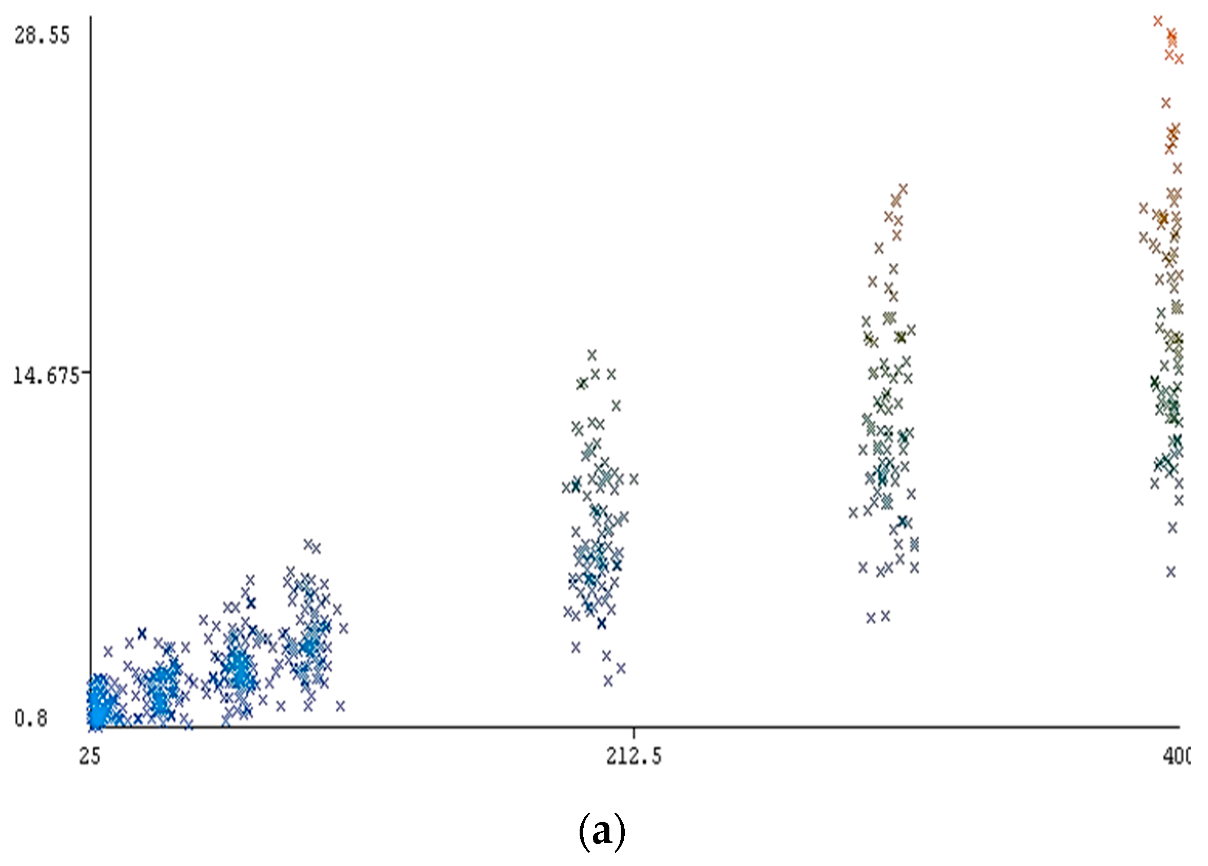

Figure 4.
Scheme of development of the database and selected methodology.

Figure 5.
The results of correlation obtained for the training datasets after conducting various models in predicting safety factor (a) Gaussian processes regression, (b) multiple linear regression, (c) multi-layer perceptron, (d) simple linear regression, (e) support vector regression.
Figure 5.
The results of correlation obtained for the training datasets after conducting various models in predicting safety factor (a) Gaussian processes regression, (b) multiple linear regression, (c) multi-layer perceptron, (d) simple linear regression, (e) support vector regression.
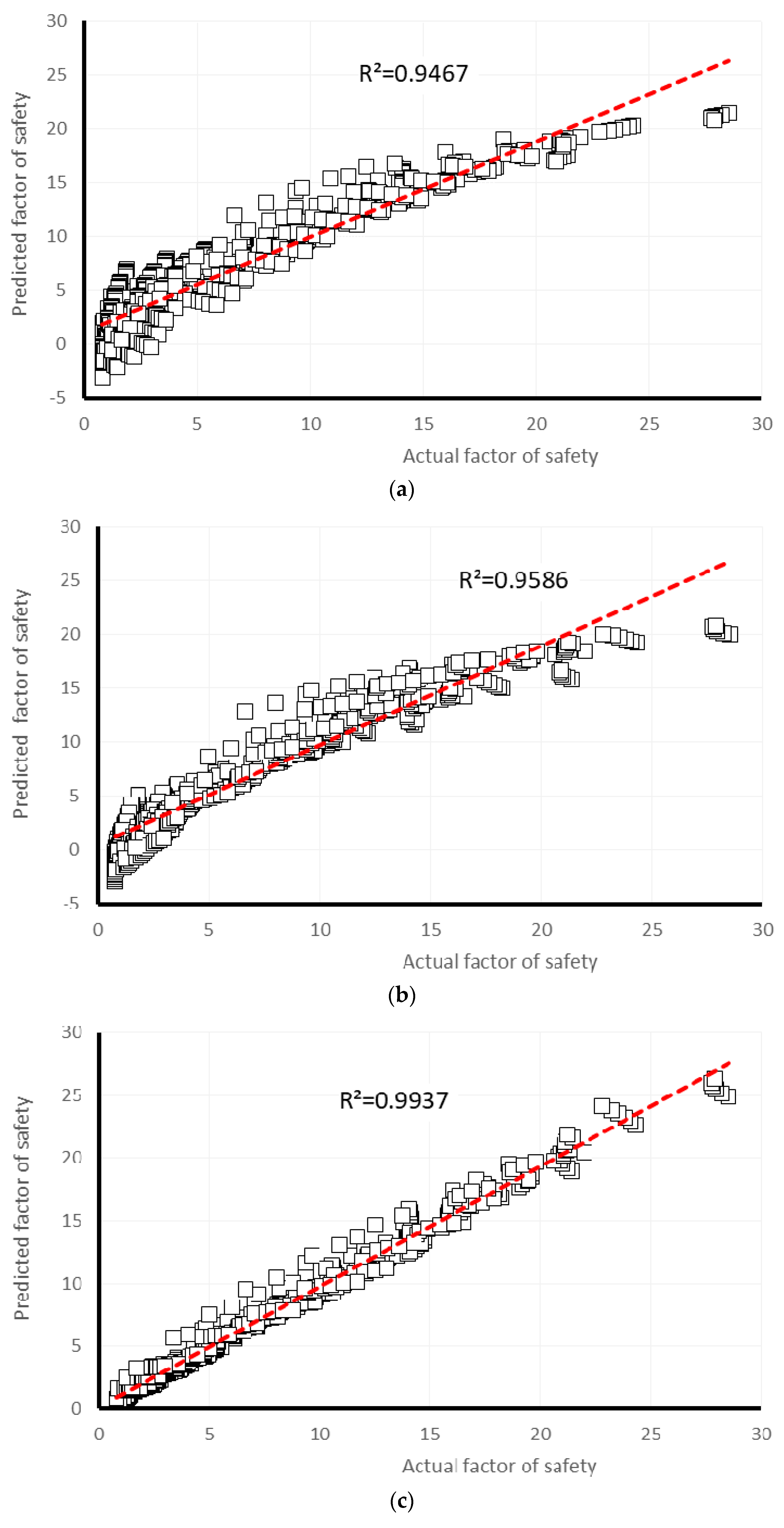

Figure 6.
The results of correlation obtained for the testing datasets after conducting various models in predicting safety factor: (a) Gaussian processes regression, (b) multiple linear regression, (c) multi-layer perceptron, (d) simple linear regression, (e) support vector regression.
Figure 6.
The results of correlation obtained for the testing datasets after conducting various models in predicting safety factor: (a) Gaussian processes regression, (b) multiple linear regression, (c) multi-layer perceptron, (d) simple linear regression, (e) support vector regression.


Figure 7.
Comparison of the errors obtained from the proposed models.
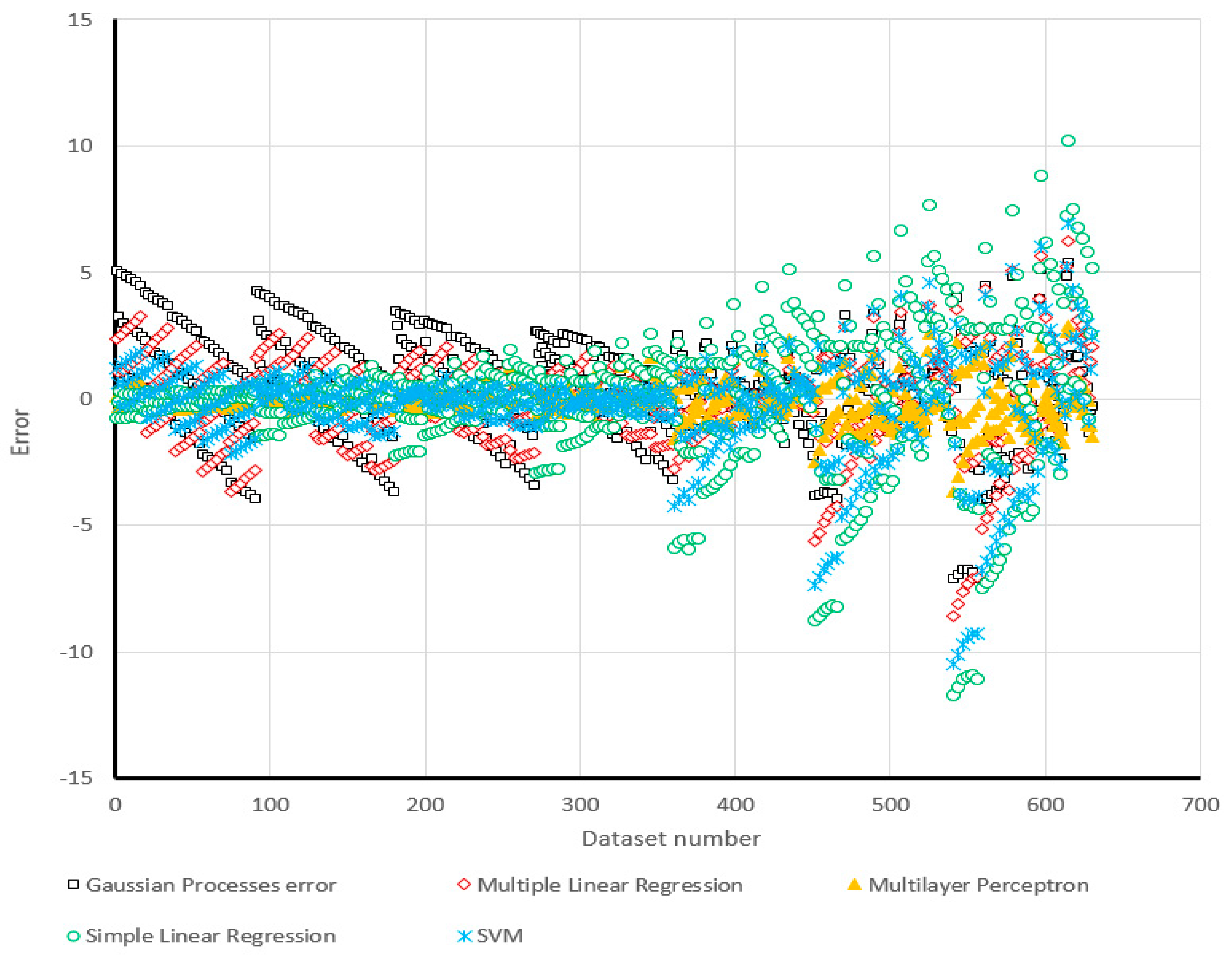
Figure 8.
Comparison of the MLP estimation and real values of FS for the β = 15°, (a) b/B = 0, (b) b/B = 1, (c) b/B = 2, (d) b/B = 3, (e) b/B = 4, (f) b/B = 5.
Figure 8.
Comparison of the MLP estimation and real values of FS for the β = 15°, (a) b/B = 0, (b) b/B = 1, (c) b/B = 2, (d) b/B = 3, (e) b/B = 4, (f) b/B = 5.

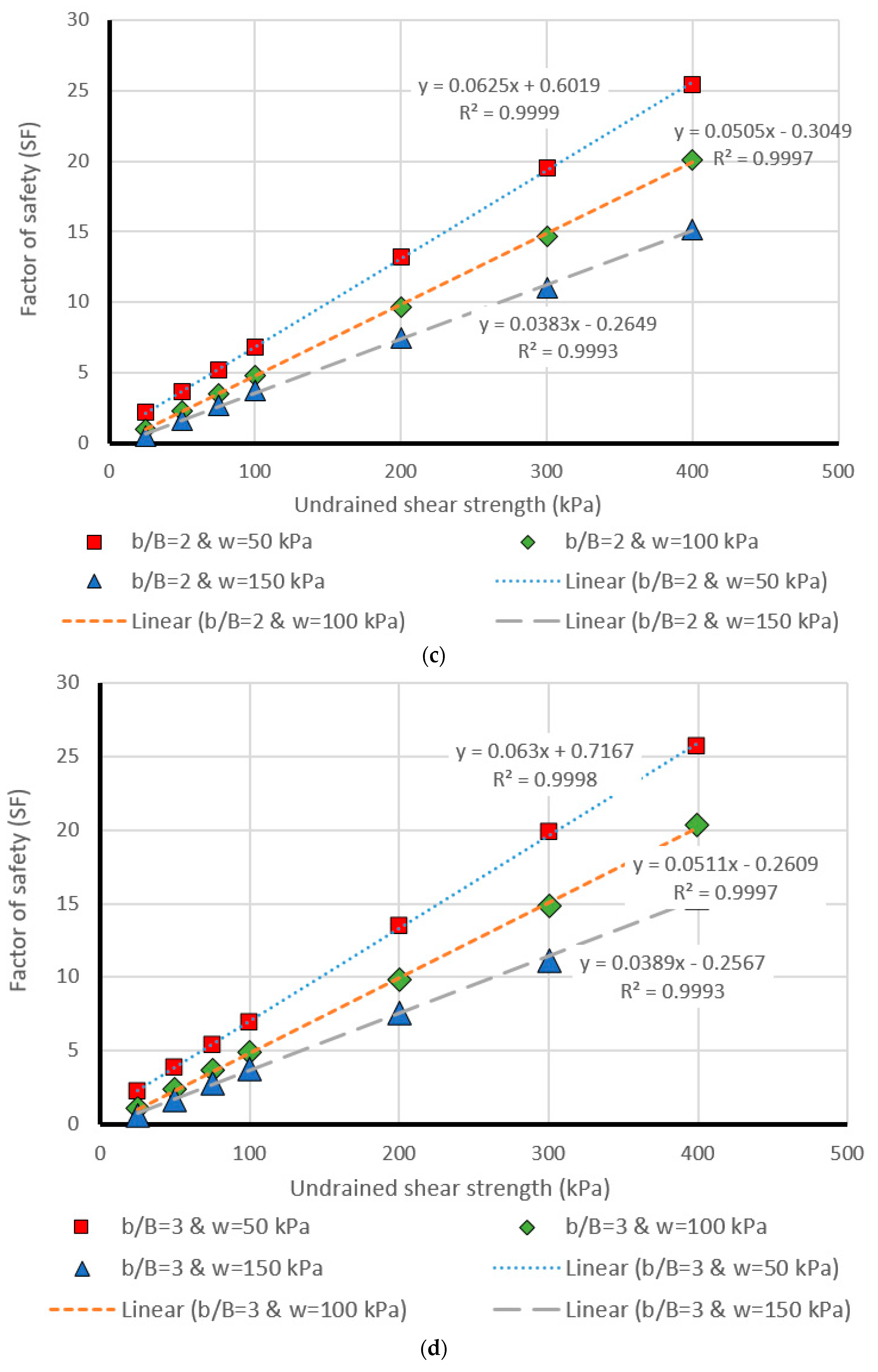
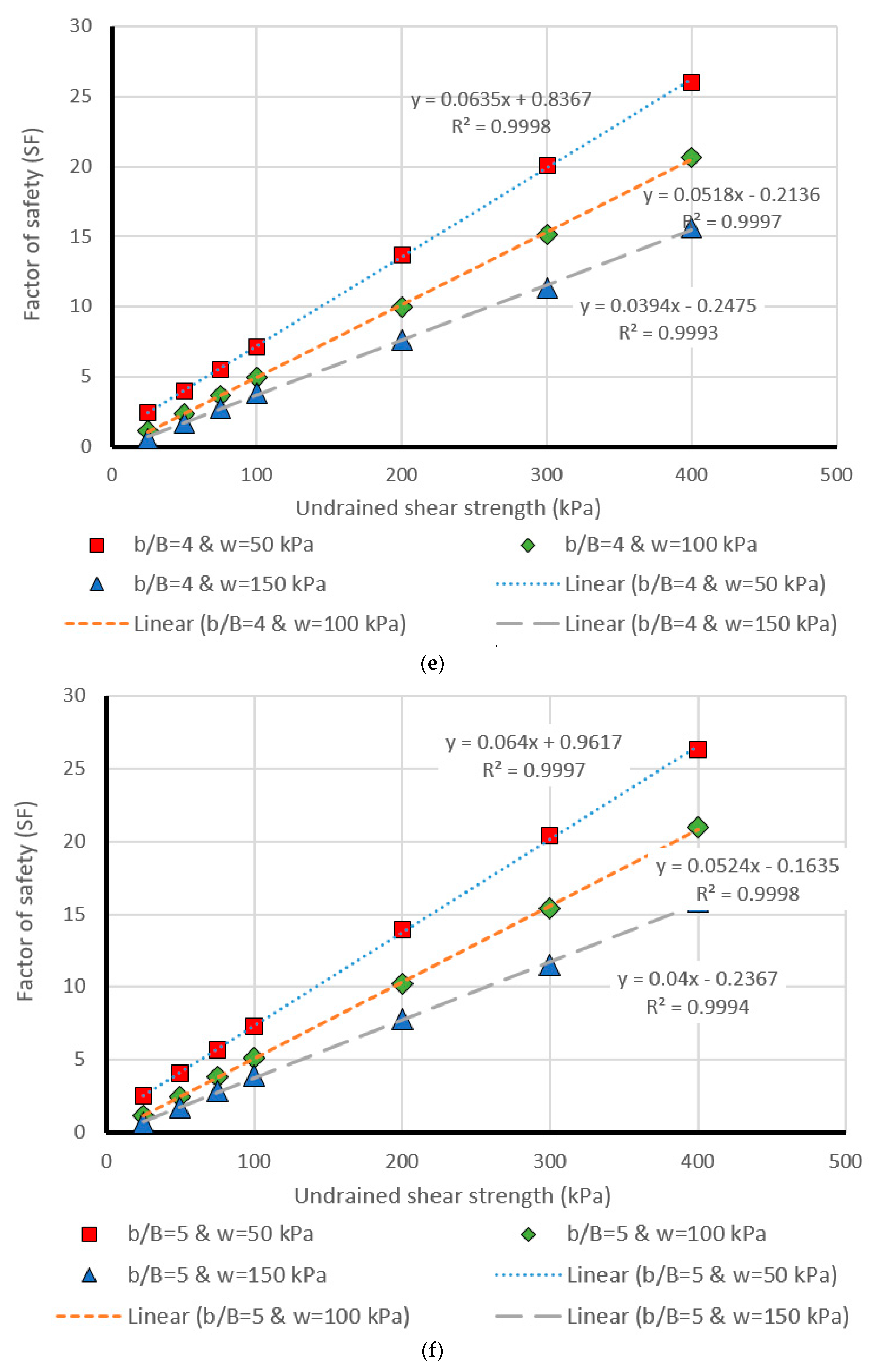
Figure 9.
Comparison of the MLP estimation and real values of FS for the β = 30°, (a) b/B = 0, (b) b/B = 1, (c) b/B = 2, (d) b/B = 3, (e) b/B = 4, (f) b/B = 5.
Figure 9.
Comparison of the MLP estimation and real values of FS for the β = 30°, (a) b/B = 0, (b) b/B = 1, (c) b/B = 2, (d) b/B = 3, (e) b/B = 4, (f) b/B = 5.
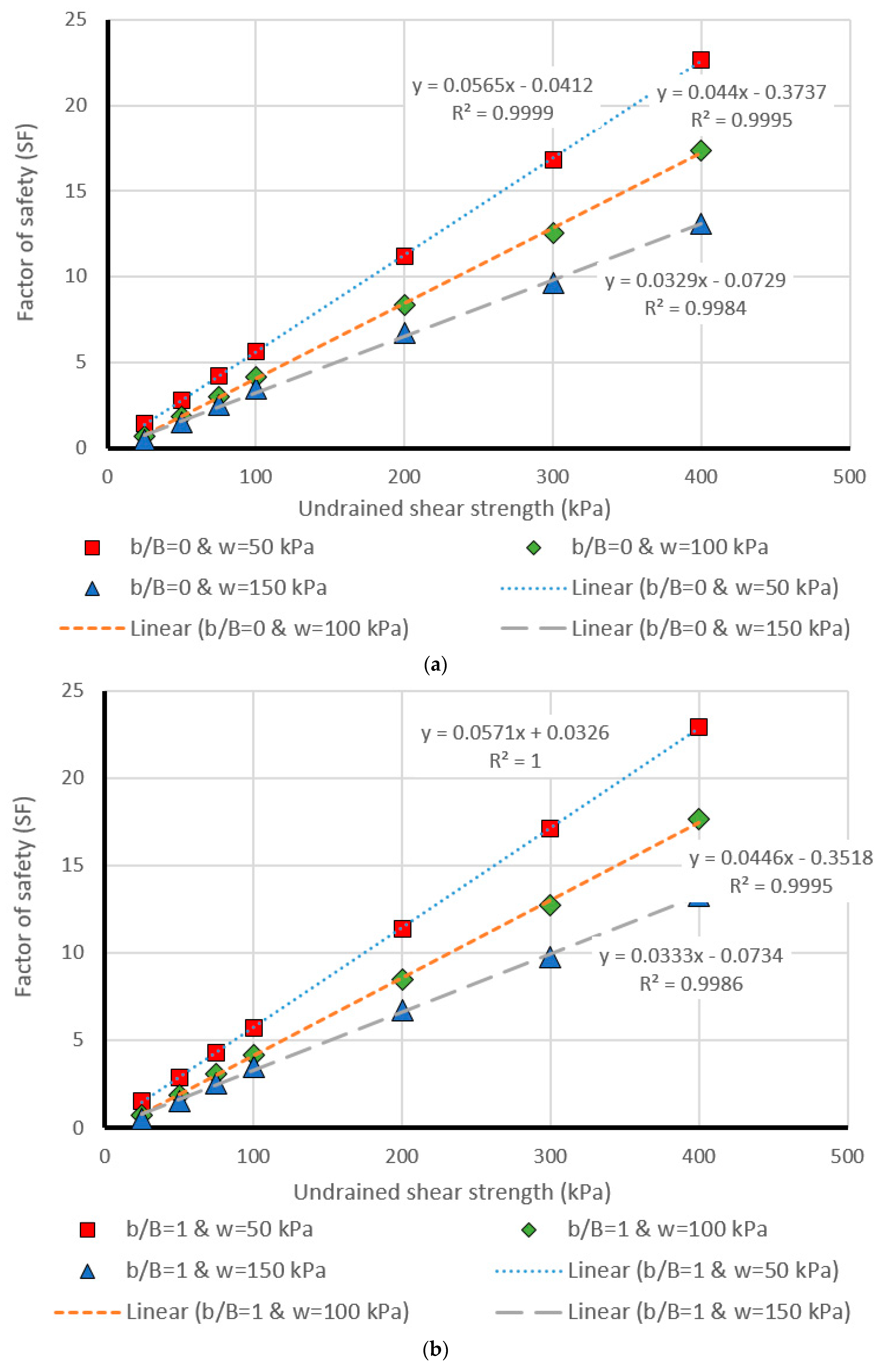


Figure 10.
Comparison of the MLP estimation and real values of FS for the β = 45°, (a) b/B = 0, (b) b/B = 1, (c) b/B = 2, (d) b/B = 3, (e) b/B = 4, (f) b/B = 5.
Figure 10.
Comparison of the MLP estimation and real values of FS for the β = 45°, (a) b/B = 0, (b) b/B = 1, (c) b/B = 2, (d) b/B = 3, (e) b/B = 4, (f) b/B = 5.
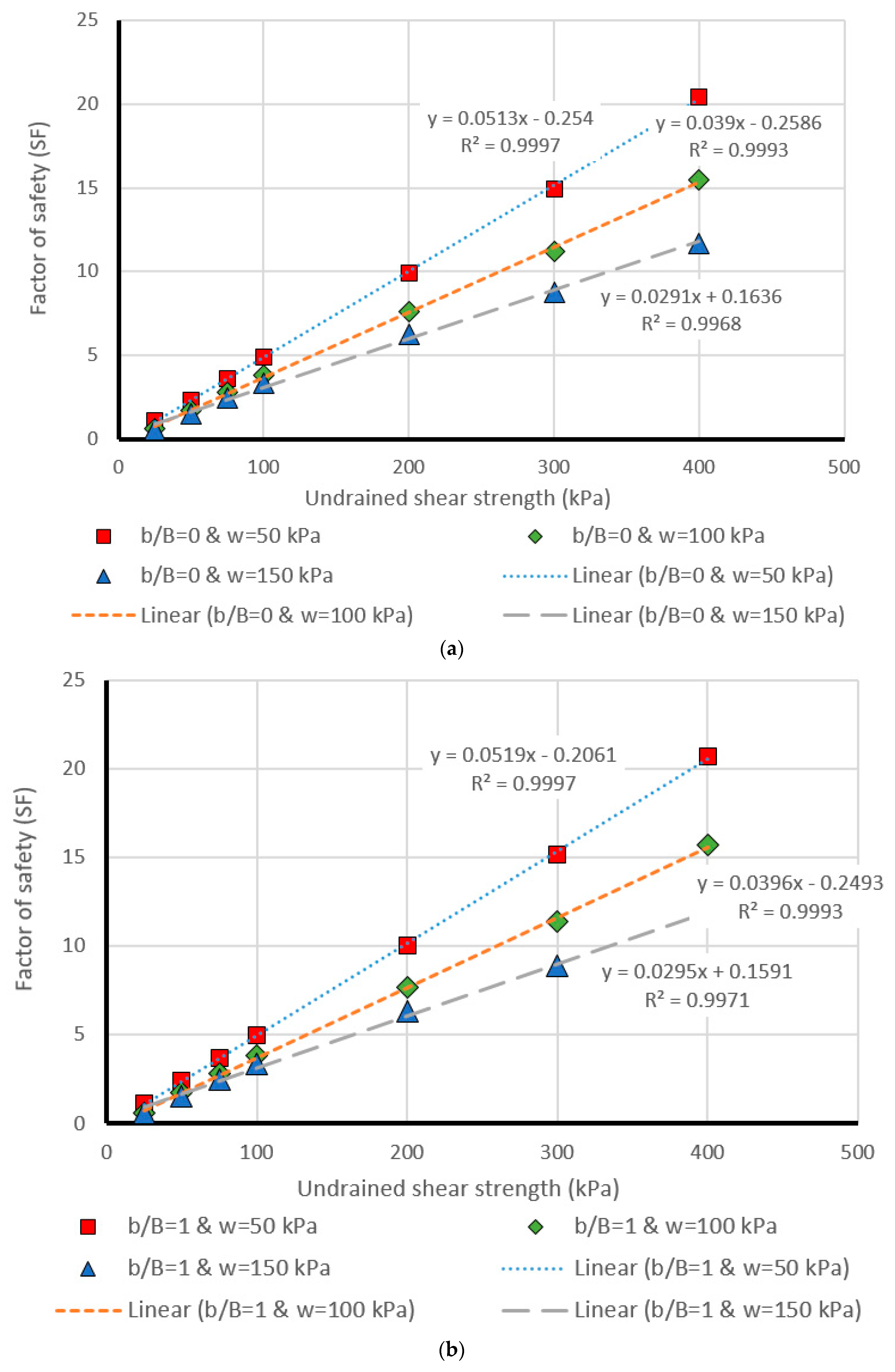
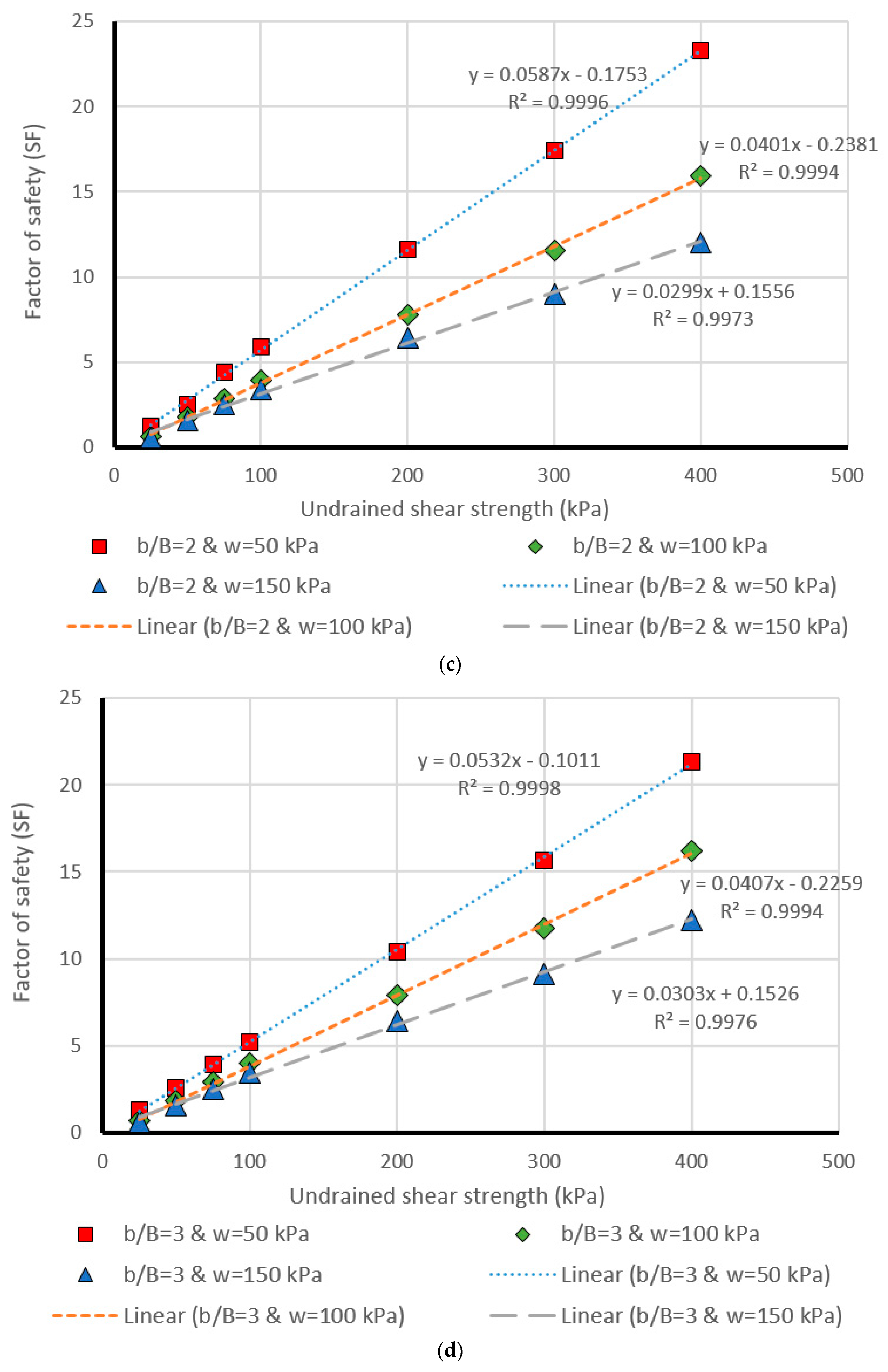

Figure 11.
Comparison of the MLP estimation and real values of FS for the β = 60°, (a) b/B = 0, (b) b/B = 1, (c) b/B = 2, (d) b/B = 3, (e) b/B = 4, (f) b/B = 5.
Figure 11.
Comparison of the MLP estimation and real values of FS for the β = 60°, (a) b/B = 0, (b) b/B = 1, (c) b/B = 2, (d) b/B = 3, (e) b/B = 4, (f) b/B = 5.
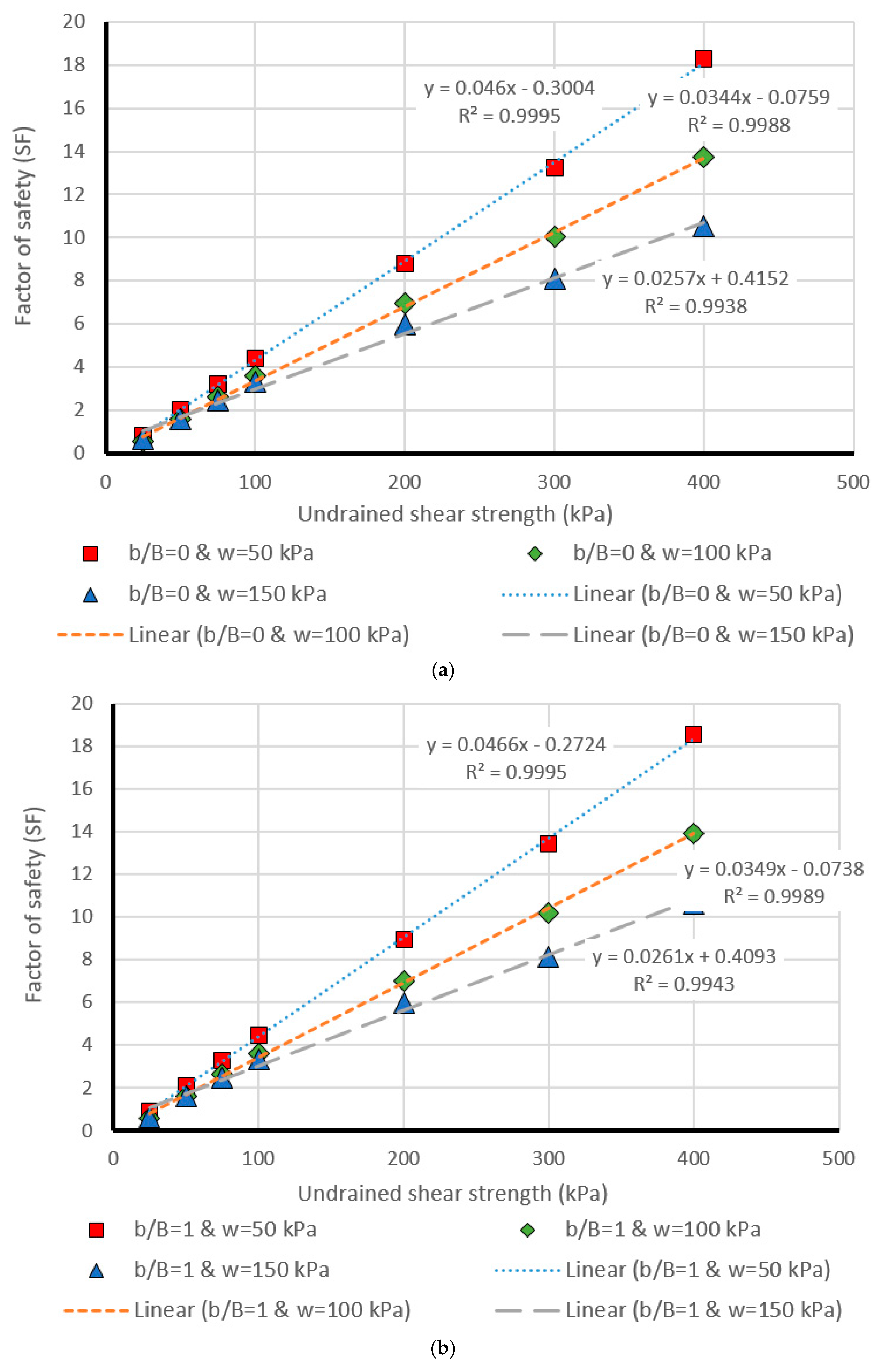
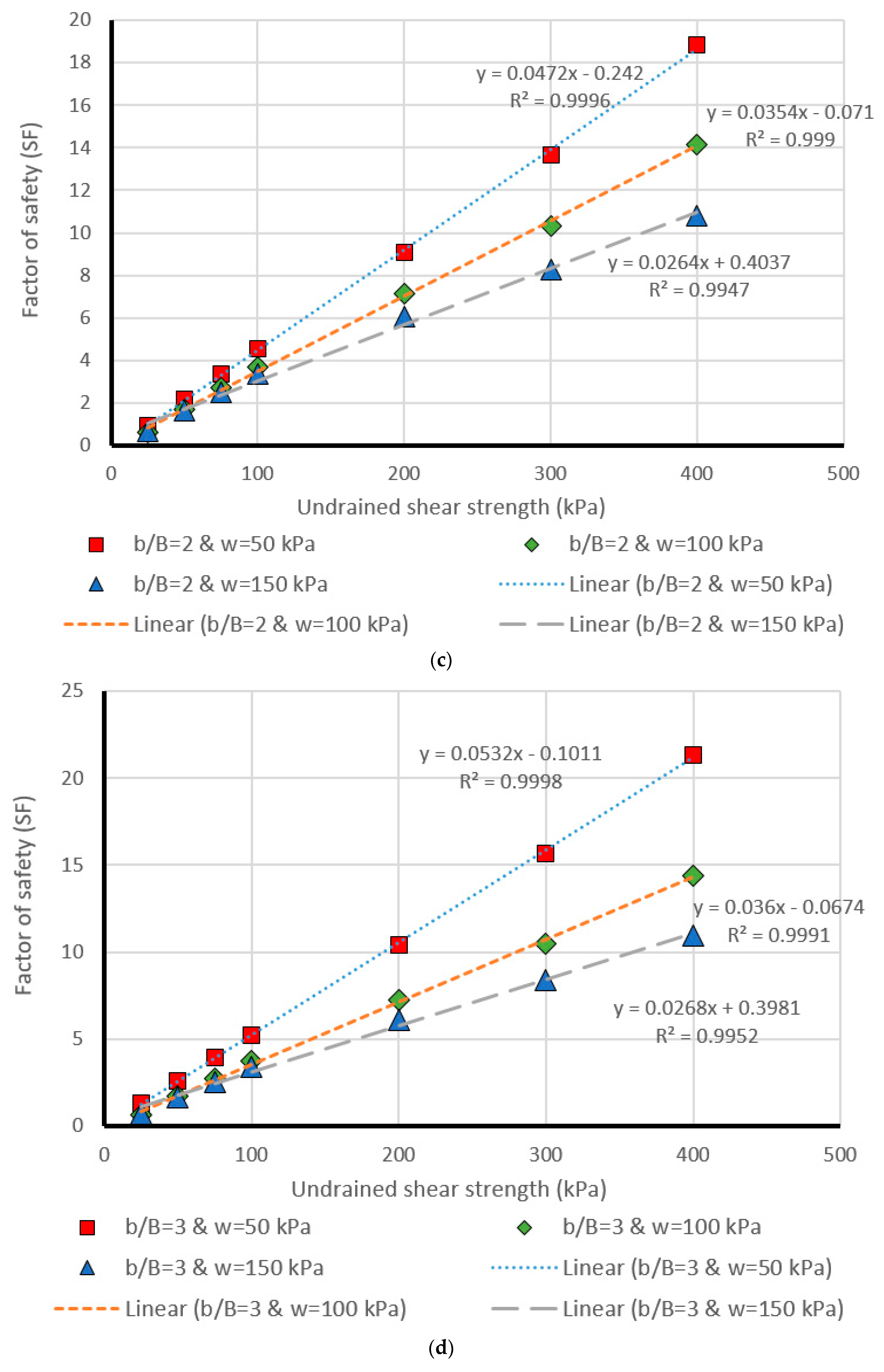
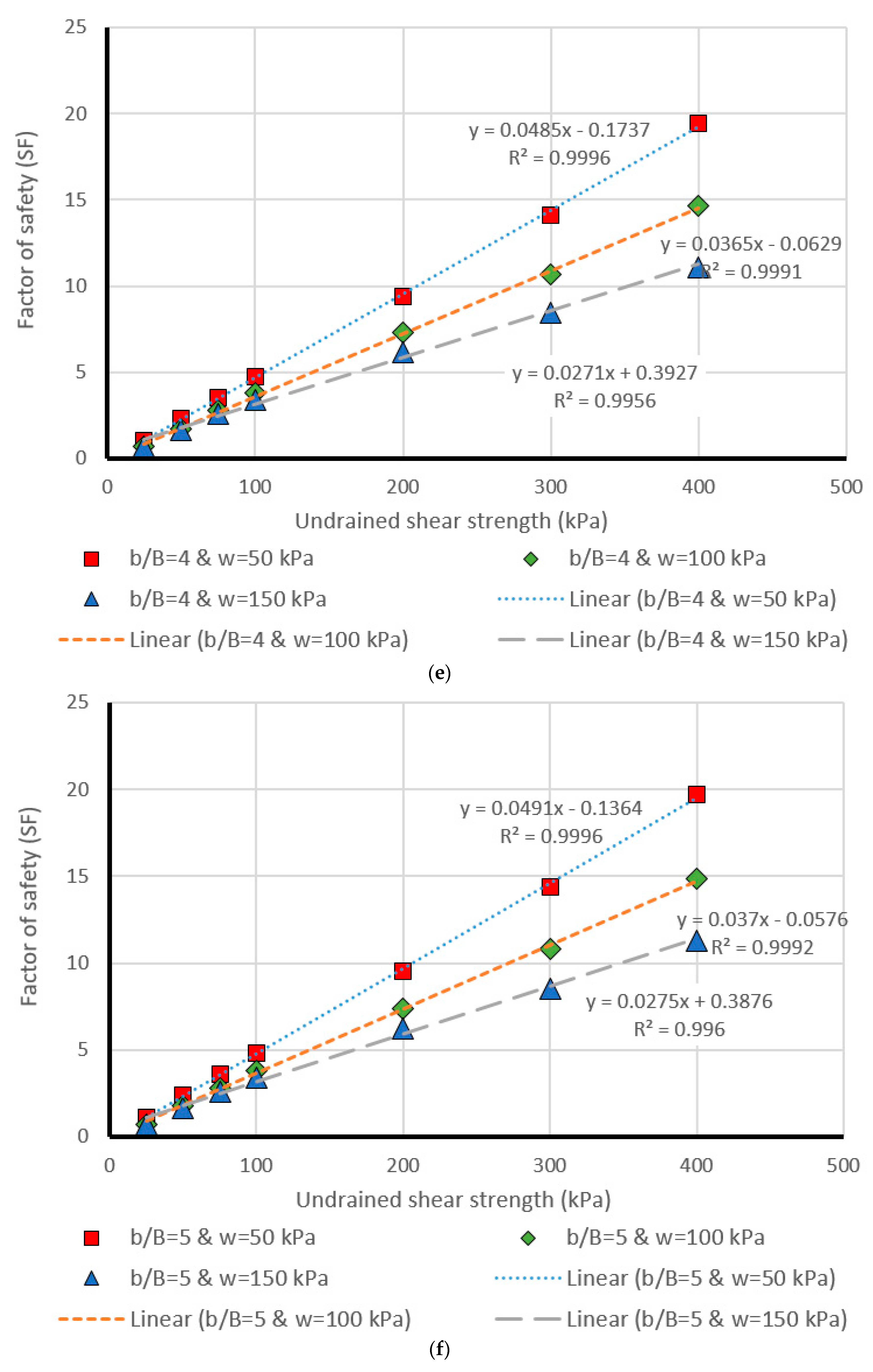
Figure 12.
Comparison of the MLP estimation and real values of FS for the β = 75°, (a) b/B = 0, (b) b/B = 1, (c) b/B = 2, (d) b/B = 3, (e) b/B = 4, (f) b/B = 5.
Figure 12.
Comparison of the MLP estimation and real values of FS for the β = 75°, (a) b/B = 0, (b) b/B = 1, (c) b/B = 2, (d) b/B = 3, (e) b/B = 4, (f) b/B = 5.


Table 1.
Total ranking of training dataset in predicting the factor of safety.
| Proposed Models | Network Results | Ranking the Predicted Models | Total Ranking Score | Rank | ||||||||
|---|---|---|---|---|---|---|---|---|---|---|---|---|
| R2 | MAE | RMSE | RAE (%) | RRSE (%) | R2 | MAE | RMSE | RAE (%) | RRSE (%) | |||
| Gaussian Processes | 0.9467 | 1.5598 | 1.9957 | 31.1929 | 32.7404 | 2 | 2 | 2 | 2 | 2 | 10 | 4 |
| Multiple Linear Regression | 0.9586 | 1.2527 | 1.7366 | 25.0515 | 28.4887 | 4 | 3 | 4 | 3 | 4 | 18 | 2 |
| Multi-layer Perceptron | 0.9937 | 0.494 | 0.7131 | 9.8796 | 11.6985 | 5 | 5 | 5 | 5 | 5 | 25 | 1 |
| Simple Linear Regression | 0.9019 | 1.7013 | 2.6334 | 34.0224 | 43.2016 | 1 | 1 | 1 | 1 | 1 | 5 | 5 |
| Support Vector Regression | 0.9529 | 1.161 | 1.9183 | 23.2182 | 31.4703 | 3 | 4 | 3 | 4 | 3 | 17 | 3 |
Table 2.
Total ranking of the testing dataset in predicting the factor of safety.
| Proposed Models | Network Results | Ranking the Predicted Models | Total Ranking Score | Rank | ||||||||
|---|---|---|---|---|---|---|---|---|---|---|---|---|
| R2 | MAE | RMSE | RAE (%) | RRSE (%) | R2 | MAE | RMSE | RAE (%) | RRSE (%) | |||
| Gaussian Processes | 0.9509 | 1.5291 | 1.9447 | 30.9081 | 32.3841 | 2 | 2 | 2 | 2 | 2 | 10 | 4 |
| Multiple Linear Regression | 0.9649 | 1.1949 | 1.5891 | 24.1272 | 26.4613 | 3 | 3 | 4 | 3 | 4 | 17 | 3 |
| Multi-layer Perceptron | 0.9939 | 0.5155 | 0.7039 | 10.4047 | 11.8116 | 5 | 5 | 5 | 5 | 5 | 25 | 1 |
| Simple Linear Regression | 0.9265 | 1.5387 | 2.2618 | 31.0892 | 37.6639 | 1 | 1 | 1 | 1 | 1 | 5 | 5 |
| Support Vector Regression | 0.9653 | 1.0364 | 1.6362 | 20.9366 | 27.247 | 4 | 4 | 3 | 4 | 3 | 18 | 2 |
Table 3.
Total ranking of both training and testing dataset in predicting the factor of safety.
| Proposed Models | Network Result | Total Rank | |||||||||
|---|---|---|---|---|---|---|---|---|---|---|---|
| Training Dataset | Testing Dataset | ||||||||||
| R2 | MAE | RMSE | RAE (%) | RRSE (%) | R2 | MAE | RMSE | RAE | RRSE | ||
| Gaussian Processes | 2 | 2 | 2 | 2 | 2 | 2 | 2 | 2 | 2 | 2 | 20 |
| Multiple Linear Regression | 4 | 3 | 4 | 3 | 4 | 3 | 3 | 4 | 3 | 4 | 35 |
| Multi-layer Perceptron | 5 | 5 | 5 | 5 | 5 | 5 | 5 | 5 | 5 | 5 | 50 |
| Simple Linear Regression | 1 | 1 | 1 | 1 | 1 | 1 | 1 | 1 | 1 | 1 | 10 |
| Support Vector Regression | 3 | 4 | 3 | 4 | 3 | 4 | 4 | 3 | 4 | 3 | 35 |
Notes: R2: Correlation coefficient; MAE: Mean absolute error; RMSE: Root mean squared error; RAE: “Relative absolute error”. RRSE: Root relative squared error.
© 2019 by the authors. Licensee MDPI, Basel, Switzerland. This article is an open access article distributed under the terms and conditions of the Creative Commons Attribution (CC BY) license (http://creativecommons.org/licenses/by/4.0/).
Share and Cite
MDPI and ACS Style
Tien Bui, D.; Moayedi, H.; Gör, M.; Jaafari, A.; Foong, L.K. Predicting Slope Stability Failure through Machine Learning Paradigms. ISPRS Int. J. Geo-Inf. 2019, 8, 395. https://doi.org/10.3390/ijgi8090395
AMA Style
Tien Bui D, Moayedi H, Gör M, Jaafari A, Foong LK. Predicting Slope Stability Failure through Machine Learning Paradigms. ISPRS International Journal of Geo-Information. 2019; 8(9):395. https://doi.org/10.3390/ijgi8090395
Chicago/Turabian StyleTien Bui, Dieu, Hossein Moayedi, Mesut Gör, Abolfazl Jaafari, and Loke Kok Foong. 2019. "Predicting Slope Stability Failure through Machine Learning Paradigms" ISPRS International Journal of Geo-Information 8, no. 9: 395. https://doi.org/10.3390/ijgi8090395
Note that from the first issue of 2016, this journal uses article numbers instead of page numbers. See further details here.