Classification of Areas Suitable for Fish Farming Using Geotechnology and Multi-Criteria Analysis

Abstract

This study proposed a method for identifying areas appropriate for fish farming in ground-excavated ponds using data obtained from public institutions. The method was applied to three cities located in the central-southern region of Paraná State, Brazil. In order to select appropriate areas, a geographic information system (GIS) was created using data from a digital elevation model (DEM), as well as data on soil occupation and type. A variable reclassification model (VRM) was created, and the analytic hierarchy process (AHP) method was applied to establish weights for a multi-criteria assessment of the factors. Non-classifiable areas and areas with constraints were identified and removed from the analysis. The sites classified as highly suitable or suitable represented 33.270.79 ha (18.71% of the total area), while the restricted areas represented 54,427.91 ha (30.60% of the total area). This method may represent a useful tool for decision making in the context of regional planning and may be used in the establishment of public policy and in the allocation of resources for aquaculture development.

1. Introduction

Among the various industries within aquaculture, fish farming is one of the most commonly practiced activities worldwide. It consists of the raising of juvenile or adult fish and typically involves an area consisting of a dammed pool of water in which the entrance and exit of water is controlled, such as a nursery, tank, pond, paddy field, or reservoir. The production systems used in ground-excavated ponds are classified as extensive, semi-intensive, or intensive [1]. Classifications of excavated ponds depend on the technological maturity of the enclosure, the equipment used, and the elements of construction used to optimize farm management [2].

Fish farming has developed over time and is now seen as a principal source of fish protein to meet current and future demands [3]. In Brazil, fish farming is in a stage of expansion and has the potential for continued growth supported by the water and land resources available, the country’s favorable climate, and producers’ entrepreneurship. In 2017, the Brazilian state of Paraná received attention for its fish production because of the state’s considerable increase in harvested fish production, particularly in the western region of the state, where the industry is supported by increased infrastructure [4].

However, in many cases, fish farms are established at inappropriate sites; this issue involves the construction of ground-excavated ponds, as well as to other situations that can compromise fish yield. Oliveira [5] defines ground-excavated ponds as artificial irrigated reservoirs on original ground with mechanisms for water filling and drainage that can be applied rapidly. Based on this definition, a suitable site is essential for avoiding negative effects on the environment and for improving pond production.

Geotechnology is useful in the selection of sites for ground-excavated ponds in that it aids in planning and optimization [6] and can be used to identify areas that are suitable for human activities such as aquaculture. According to Malczewski [7], a multi-criteria approach can be used to obtain effective geoprocessing results when geographic information systems (GIS) are integrated into it; this technique represents a significant advancement over conventional procedures for prioritizing specific areas. In this approach, the basis for the decision making lies in the criteria and sub-criteria, which may be represented by both factors and constraints.

These multi-criteria analysis methods were first introduced in 1970. Before they were available, the optimization methods used to aid in decision making were based on mathematical programming equations and had the goal of solving only a single objective function [8]. It is also important to note that the aquaculture industry has typically relied on manual labor to outline areas suitable for aquaculture, a process which is slow and which limits coverage only to a sample area. Therefore, the classic optimization method is not able to combine all of the criteria to determine a single result [8].

Multi-criteria analysis was developed as a result of the need to analyze problems from different perspectives and to study many different criteria at once. This method seeks to provide multiple solutions to an issue as a function of different criteria, which, in many cases, are conflicting [9]. Among the various methods in which multi-criteria analyses are employed, the analytic hierarchy process (AHP) developed by Saaty [10], is a practical and useful method to aid in decision making that guarantees consistency across all of the options considered. It can be applied to various industries and fields of research because it considers both qualitative and quantitative information and compiles this information into a hierarchical structure in which weights and priorities are derived on a ratio scale in order to make pair-by-pair comparisons to measure the degree of importance of the criteria and sub-criteria established and, in doing so, to determine a normalized set of weights to be used [11,12].

Some important characteristics of the region chosen for this study include its high level of social inequality and its low human development index (HDI) score relative to the surrounding regions. Family farming is the main economic activity in this region; the average property size is less than 50 ha [13]. Perussato et al. [14] cite that fish farming in ground-excavated ponds has become an important option for agricultural production systems, particularly for small rural farmers who rely on family labor; it is therefore very important that the sites most suitable for this activity be identified. According to a local supply chain and land use report known as the PTCP, fish farming in this region is in its infancy when compared to the scale of other supply chains. This conclusion was based on the amount of variation and inconsistency in the fish farming sites established in the region [15].

The objective of this study was therefore to propose the creation of a method to classify and identify areas suitable for fish farming in ground-excavated ponds. The identification and classification process relied on data obtained from official government institutions and considered geological factors (soil type), geomorphological factors (slope and altitude), and current soil use and occupation in three cities in Paraná State in Brazil.

2. Materials and Methods

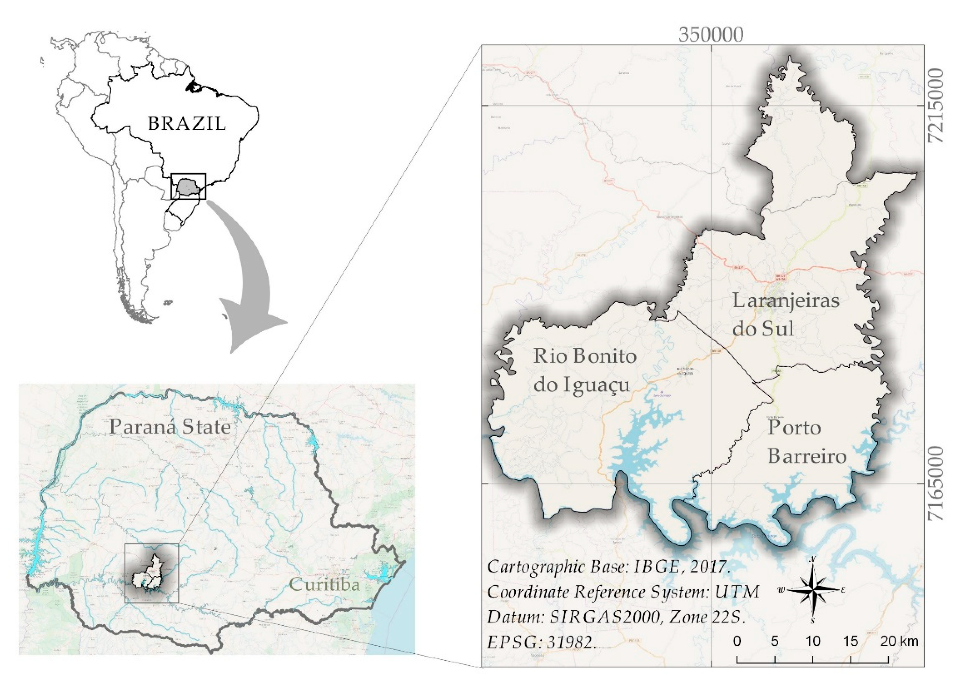
2.1. Study Area

The study area consisted of three cities located in the microregion of Guarapuava, located in the central-southern region of Paraná State, Brazil: Laranjeiras do Sul, Rio Bonito do Iguaçu, and Porto Barreiro, as shown in Figure 1. According to the Köppen climate classification system, the cities are located in a Cfb climate region, represented by a temperate climate with mild summers [16]. The region was chosen because fish are not commercially produced there and because its economy is largely structured around family farming.

2.2. Workflow

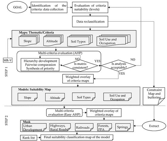
In the suitability classification of fish farming areas, a multi-criteria analysis was integrated into a GIS environment to aid in the selection of the most suitable sites for fish farming in ground-excavated ponds. The method consisted of a set of sequential analytical steps presented in the workflow in Figure 2.

2.2.1. Step 1

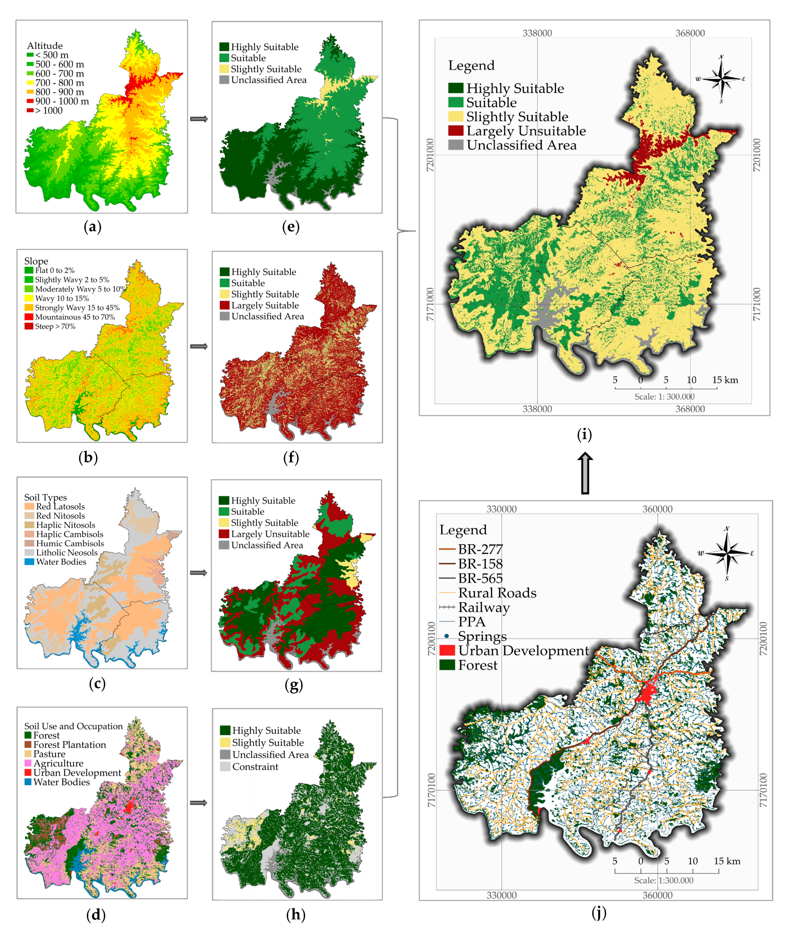
• Criteria were identified based on the data obtained, and a GIS database was developed to present the spatial distribution of the factors involved and to determine the suitability.
• A variable reclassification model (VRM) was constructed to make the reclassification of the initial data more flexible for the creation of thematic maps and suitability scale maps.
• Procedures were performed to determine the consistency of the matrix and to determine whether the analysis was acceptable or not; when it was, the model was constructed.
• A paired comparison matrix was created for the models (suitability maps) using the intensity scale of importance provided by Saaty [10]. To attribute the respective weights of importance, the researchers’ prior knowledge as specialists in the field and a review of the literature were used to make the judgements necessary to create the matrix.

2.2.2. Step 2

• After the classification and generation of parameters, the Easy AHP plugin in QGIS was used to calculate the relative importance (weights) of the criteria. This algorithm offers an analysis of the AHP method [17] and of the weighted linear combination (WLC) method [7].
• Based on the importance of each factor to classify and identify the areas suitable for fish farming in ground-excavated ponds, each variable was multiplied by its respective weight, and the results were added together [7] to generate a suitability classification map for fish farming.
• Areas that were considered to be restricted due to legal limitations or technical limitations were identified spatially, and a specified buffer distance was applied around the features for their subsequent removal from the final map.
• The priorities of the criteria and sub-criteria were ranked in order to classify the sites that were most suitable for fish farming according to the determined criteria.

2.3. Data Acquisition

The creation of this method began with the acquisition of the city limits and subdistrict limits relevant to this study, which were obtained from maps on a 1:250,000 scale from the Brazilian Institute of Geography and Statistics (IBGE) website in shapefile vector data format (shp). To obtain data on the local freshwater and surface water system, a digital file on a 1:50,000 scale was obtained from the Paraná State Department of Water Resources containing information on the courses of local rivers. Aa part of this step, these courses were divided into sections connected by nodes and identified by unique hierarchical codes following the methods used by the Brazilian National Water Agency (ANA) and the method provided by Otto Pfafstetter [19].

Information on the topographical relief of the region was obtained using a digital elevation model (DEM) and maps generated to show altitude and slope based on Shuttle Radar Topography Mission (SRTM) data (version 3, band C, with a spatial resolution of 1 arc-second, or approximately 30 m). This information on land elevation was processed and distributed by the United States Geological Survey (USGS). The information was distributed into classes through the use of the r.reclass algorithm in QGIS in order to improve the topographical display of the region. The slope classes were established as flat (0–2%), slightly wavy (2–5%), moderately wavy (5–10%), wavy (10–15%), strongly wavy (15–45%), mountainous (45–70%), and steep (greater than 70%) (Lepsch et al., 1991). Arbitrary colors were used to aid in the visualization and interpretation of the results. The altitude map was also classified into seven classes with a 100 m difference between each class.

The vector data on the map in shp format containing the most common soil units was obtained directly from the Brazilian Agricultural Research Corporation (EMBRAPA), which has a series of maps referred to as the Maps of Soils from the State of Paraná [20] on a 1:250,000 scale. For the reclassification, second-level classes (suborders) were considered, the soil map was edited to include only the area of interest, and the soil types were identified.

Data on soil use and occupation were obtained from the Mapbiomas Collection as raster data in GeoTIFF format on a 1:100,000 scale and at a spatial resolution of 30 m [21]. The Mapbiomas project involves researchers and specialists in remote sensing, computer science, biome science, and the most common uses of soil in Brazil.

It is important to note, that all of this data was obtained free of charge from open-source data, from government websites, and from other institutions websites. All of the data contained in the database required treatment and reclassification to create thematic layers and to record each layer in order to then create a single system of coordinates.

2.4. Standardization of Spatial Data

All of the spatial data were re-projected in the official geodetic datum of Brazil, known as SIGRAS2000 (Sistema de Referência Geocêntrico para as Américas, 2000) in a UTM projection (Zone 22 South) as established by the Brazilian Institute of Geography and Statistics (IBGE). All of the raster files were converted into a single configuration: a spatial resolution with 30 m pixels, an unsigned 8-bit datatype, consistent column and row dimensions (1909 and 2180 pixels, respectively), and with no null pixel values through operations performed in QGIS. These steps were performed in order to facilitate the operations involving metric quantification and to standardize the parameters of the matrix data in order to then perform the multi-criteria analysis. The variety of scales in which all of the criteria were measured was considered, because this analysis requires that the values contained in the different layers be transformed into the same unit of measurement [22]. The procedures performed on the map were carried out in matrix format. However, to improve the visual presentation and to represent the features as smoothly as possible, the data in matrix format were converted into vector data, making the file sizes considerably smaller, since the quantity of vertices decreased. All of the vector bases underwent topological validation in order to maintain the integrity and quality of the spatial data information.

2.5. Software

The spatial data were analyzed in a GIS platform using the QGIS Noosa software, version 3.6.3, which is a free and open source and which has an intuitive interface, all of which allowed for the unrestricted progress of the research performed herein. The parameters studied were inserted and spatially manipulated. The information was organized in its database into information plans (IPs) and was manipulated by logical and mathematical operators. Each IP is presented as a type of map, and also as a direct instance of the category to which it belongs [23].

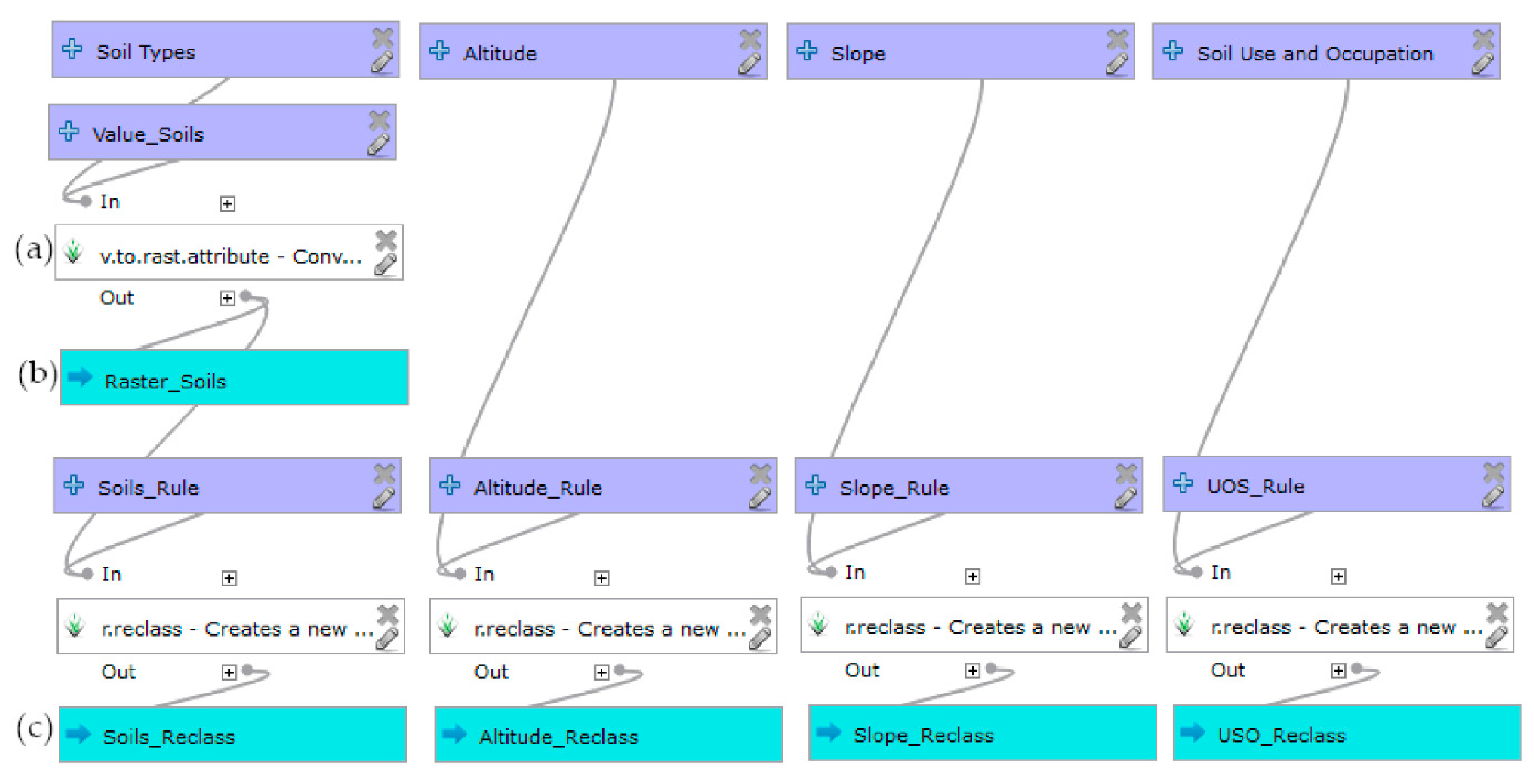
2.6. Variable Reclassification Model (VRM)

To optimize the procedure, a VRM was first constructed using the variables (slope, altitude, soil type, and soil use and occupation) and the IP creation process provided by [24], with modifications (Figure 3). For this step, the QGIS graphical modeler was used (available in the Processing Menu). The reclassification rules were inserted using Notepad in the r.reclass algorithm format in QGIS for the construction of thematic maps and suitability scale maps.

After the result was saved, the parameters of the algorithms used in the model were filled in, and the values of the original pixels were replaced by the values attributed to the reclassification rules, as defined during the construction of the thematic maps and the suitability scale maps. The parameters of the model were filled in, as shown in Figure 4.

This model was created to streamline and optimize the process and to meet the demand for the reclassification of these variables. According to Rezende et al. [24], this model may be applied to other studies that have many variables and classes, and it has the advantage of reducing the processing time and the number of possible errors.

2.7. The AHP Method

Multiple-criteria decision analysis was established as a concept with corresponding terminology by Roy [25], who developed the ELECTRE family of multi-criteria decision analysis methods and, in doing so, gave rise to the French school of decision making. The AHP methods and variations therein were developed by Saaty [10] and became the reference for the American school of decision making [26]. The AHP method was used in this study because it allows its users (specialists) to attribute weights to multiple attributes or to attribute multiple options to one attribute while performing a paired comparison between them [17]. Furthermore, the method considers the influence and effects of these criteria and has a judgement scale that defines the importance of a set of criteria [27].

2.7.1. Suitability Classification and Scores

A procedure was created to establish a score for each criterion in the model. These criteria were reclassified and scored, as shown in

Table 1. Classification of suitability and scores for the suitability model.

Suitability Model	Suitability Classification and Scores
	Highly Suitable a (4)	Suitable b (3)	Slightly Suitable c (2)	Largely Unsuitable d (1)	References
Slope	≤2	>2 ≤ 5	>5 ≤ 10	>10	Adapted from Giap et al. [30]; Falconer et al. [28]
Altitude	≤700	>700 ≤ 900	>900	-	Adapted from Coelho & Torres [31]; McLeod et al. [32]
Soil Type	RL	RN HN	HC UC	LN	Adapted from Scheleder & Skrobot [33]; Ono & Kubtiza [34]
Soil Use and Occupation	Agriculture Pasture	-	Forest Plantation	-	Adapted from Völcker & Scott [23]

RL = Red latosols; RN = Red nitosols; HN = Haplic nitosols; HC = Haplic cambisols; UC = Humic cambisols; LN = Litholic neosols; ^a Only a minimum amount of time and common investment are required for fish farming; ^b Requires a modest amount of time and investment. No construction, project, management or uncommon maintenance are needed for the designated use; ^c This category indicates that there are one or more parameters that will demand special attention for the designated use, but that these issues may be overcome through projects and special maintenance; ^d This category indicates that in addition to local legal restrictions, one of more unfavorable parameters for the evaluated use, such as time, cost, or both, are too significant for fish farming to be successfully implemented.

, similar to the method used by Falconer et al. [28], in which a categorical scale was adopted. On this four-point scale, a 1 was “largely unsuitable,” a 2 was “slightly suitable,” a 3 was “suitable,” and a 4 was “highly suitable.” All of the factors were scored based on their categories using recommendations from the literature [29], as well as the authors’ experience. Therefore, to be able to classify the sites that were most suitable for fish farming, two items were considered in the evaluation of the criteria: the factors and the constraints. Nath et al. [29] argue that a factor should be understood as a measurement of the suitability of criteria in the context of the activity in question, and a constraint should be understood as a limitation on the alternatives available, or should be applied to sites where, for a variety of reasons, the activity in question may be hindered or restricted.

2.7.2. Determining Weights Using AHP

The weight of each factor was determined through a comparison of the paired matrices in the context of AHP [12]. These comparisons reflect the relative importance of the two criteria in question (

Table 2. Scale of the relative importance of two criteria ¹.

1/9

1/8

1/7

1/6

1/5

1/4

1/3

1/2

1

2

3

4

5

6

7

8

9

Extremely

Very strongly

Strongly

Moderately

Equally

Moderately

Strongly

Very strongly

Extremely

LESS IMPORTANT

MORE IMPORTANT

¹ Source: Hossain & Daz [35].

), which are established by the fish farming suitability classification map. To apply this procedure, the sum of the weights must be equal to 1 [35]. The scale of relative importance developed by Saaty [10] is an assessment scale divided into nine levels based on systematically scored classifications on a continuous seventeen-point scale on which 1/9 and 1/8 represent the least important scores and 8 and 9 represent the most important scores, as detailed in Table 2.

Using the scale of relative importance, the comparison matrix was constructed to establish the mutually important criteria. This is a squared matrix with reciprocal values in which diagonally, the values are uniform, since each variable compared to itself is equal to the unit [36]. Preferences for the implementation of fish farming in relation to the evaluation criteria were incorporated into the decision-making model to attribute the relative importance of each criterion. These criteria were classified based on literature reviews and by the professional opinions of seven specialists from different fields, including environmental oversight and fishing resources (these specialists also included professors from vocational and higher education institutions). Relative weights were attributed and referred to as “priorities” to distinguish between the levels of importance of the criteria. In this step, the intensity of the values used in the method was found to be derived from the subjective preferences of the researchers, which may result in inconsistencies in the final matrix. Therefore, to define the acceptable value for this inconsistency, the AHP calculates a consistency ratio (CR) by comparing the consistency index (CI) of the matrix in question to a random consistency index, or RI [37]. The RI is presented in

Table 3. Random Consistency Index (RI) ¹.

n	1	2	3	4	5	6	7	8	9	10
RI	0	0	0.58	0.90	1.12	1.24	1.32	1.41	1.45	1.49

¹ Source: Saaty [12].

. Saaty [12] suggests that, for there to be satisfactory consistency of the data, the result of the CR must be less than 0.10 or 10%, a value which indicates the reliability of the specialists judgement; if the result is higher than 0.10, there will be inconsistencies, and the AHP method will not produce significant results. The Easy AHP algorithm was used in QGIS to apply the weight of each factor and obtain a paired comparison matrix, as well as a CI and a CR. The results of the comparisons between pairs were organized into a matrix in which the weights of the factors were determined by the order of priority. In this order, the first (dominant) item, the normalized eigenvector, supplies the ratio scale (weight), and the eigenvalue determines the CR [38].

2.7.3. Data Integration

The AHP method [10] was combined with GIS technology to compare each of the layers of the map and to determine the values of their respective weights. The layers of the map and the values of the weights were combined using WLC. The Easy AHP plugin was used in these cases; it provided the AHP and WLC analyses in QGIS, version 3.6.3.

Five paired matrices were created to determine the suitability classification for each level of a factor; the matrices were evaluated based on the results of previous research and on the opinions of the specialists involved.

Table 4. Paired comparison matrix to evaluate the relative importance of the main criteria used to identify areas suitable for fish farming.

	Paired Comparison Matrix (A)				Normalized Comparison Matrix a				($\mathit{\omega }$) b	$\mathit{\lambda }\mathit{m}\mathit{a}\mathit{x}{ }^{\mathbf{c}}$	CI d	RI e	CR f
	S	A	T	U	S	A	T	U
S	1	3	2	7	0.506	0.474	0.541	0.438	0.4894	4.0346	0.0115
A	1/3	1	1/2	3	0.169	0.158	0.135	0.188	0.1623	4.0080	0.0027
T	1/2	2	1	5	0.253	0.316	0.270	0.313	0.2879	4.0260	0.0087
U	1/7	1/3	1/5	1	0.072	0.053	0.054	0.063	0.0604	4.0082	0.0027
∑	1.98	6.33	3.70	16					1	4.0192	0.0064	0.90	0.007

S = slope; A = Altitude; T = Soil type; U = Soil use and occup; ^a If the values of each column of the paired comparison matrix are added together and if each value in the matrix is divided by the sum of the column, the resulting matrix is the normalized comparison matrix; ^b The eigenvector ($\omega )$ is the average of the values in each line of the normalized comparison matrix and results in the score (weights); ^c The eigenvalue ($\lambda max$) results from the product of Matrix (A) multiplied by Matrix ($\omega$) and the result is obtained by dividing each line by the corresponding $\omega$ in order to obtain each ${\lambda }_i$ of a $\lambda$ estimate vector, and the approximate $\lambda max$ is the mean of the ${\lambda }_i$, resulting in $\lambda max$ = 4.0192; ^d The consistency index (CI) is calculated as ${\displaystyle \sum }\left({\lambda }_{i max}-n\right)/\left(n-1\right)$, resulting in a CI of 0.0064; ^e The random consistency index (RI), suggested by Saaty [10] for four criteria, is 0.90; ^f The consistency ratio (CR) is CI/RI, being 0.0064/0.90 = 0.007.

presents the paired matrix spreadsheet calculations for the criteria, and

Table 5. Paired comparison matrix to evaluate the relative importance of the sub-criteria used to identify areas suitable for fish farming.

Criterion		Slope (%)
Sub-Criterion	≤2	>2 and ≤5	>5 and ≤10	>10	Weight
≤2	1	1	3	7	0.4113
>2 and ≤5		1	3	5	0.3800
>5 and ≤10			1	3	0.1475
>10				1	0.0611
Consistency ratio (CR) = 0.012
Criterion		Altitude (m)
Sub-Criterion		≤700	>700 and ≤900	>900	Weight
≤700		1	2	5	0.5813
>700 and ≤900			1	3	0.2784
>900				1	0.1096
Consistency ratio (CR) = 0.009
Criterion		Soil Type
Sub-Criterion	RL	RN; HN	HC; UC	LN	Weight
RL	1	2	7	9	0.5271
RN; HN		1	5	9	0.3428
HC; UC			1	3	0.0883
LN				1	0.0418
Consistency ratio (CR) = 0.038
Criterion		Soil Use and Occupation
Sub-Criterion		Agriculture	Pasture	Forest Plantation	Weight
Agriculture		1	1	9	0.5281
Pasture			1	7	0.4274
Forest Plantation				1	0.0636
Consistency ratio (CR) = 0.015

presents the value of the paired matrix for each of the sub-criteria. Some examples of the construction of these matrices may be seen in Rekha et al. [39], Rezende et al. [24], Bagdanavičiūtė et al. [18], and Nayak, et al. [40], among others.

2.8. Ranking the Factors

The AHP method uses two types of measurement: relative and absolute. In order to create an ordered classification, absolute measurements were applied. This choice allowed for the sites most suitable for fish farming to be ranked based on specifically determined criteria. According to Teixeira [41], when this measurement is applied, only the main criteria are compared in pairs to derive their priorities, and the sub-criteria are classified only within the criteria to which they belong.

A priority scale was established after the multiplication of the weight of each criterion by the weight of its respective sub-criteria using the paired comparison matrices in Table 4 and Table 5. An ordered list of factors and all of the areas that were potentially suitable for fish farming were therefore classified within a recommended interval. To make a decision, regarding the recommended intervals, the equal interval classification method was applied to define the four classification intervals (highly suitable, suitable, slightly suitable, and largely unsuitable). The classification of the intervals (CIs) between their respective distances was calculated using Equation (1):

$$\mathrm{CIs}=\left(\mathrm{H}-\mathrm{L}\right)/4$$

(1)

where (H) is the highest classification value and (L) is the lowest classification value.

2.9. Constraints on Fish Farming Implementation

In this study, certain factors that impede or restrict the implementation of fish farms in ponds were spatially identified. Areas were considered to have constraints when there were legal restrictions or technical aspects that made fish farming unfeasible or impossible. The factors that could restrict or impede fish farming included forests, urban perimeter, highways and railways, permanent preservation areas (PPA), water springs or other sources of water, airports, dirt roads or other rural constructions, telephone poles or power lines, environmentally protected areas, or other areas where land use was restricted.

It is also important to note that this study was limited to identifying areas with the potential for fish farming in ground-excavated ponds. Though water is essential for fish farming, all of the areas with bodies of water such as rivers, channels, and lakes were not considered in the final model, because ground-excavated ponds cannot be built within a body of water. This exclusion made the estimates more effective. It is also important to note that bodies of water were not treated as a constraint on fish farming but simply as non-classified areas.

The data considered to be restricted in this study were identified spatially using specific QGIS routines and the buffer function. Next, all of the polygons (collected geometries) were merged into a single file (the mask IP). Next, a command line was used in GDAL within QGIS to perforate the suitability classification map. To perforate the desired image, the following command line was used through OSGeo4w (an open-source Windows installer for GIS projects): gdal_rasterize -b 1 -burn 1 mask-name.shp image-name.tif.

3. Results

3.1. Analysis and Identification of the Classification Criteria Used to Determine Sites Suitable for Fish Farming

An early step in the project was to characterize the study area. Thematic maps were created as shown in Figure 5a–d. Figure 5a presents the altitude map; the city of Laranjeiras do Sul was found to be at the highest elevation, with most of the city limits above 800 m and a small portion above 1000 m. The city of Porto Barreiro was at the second highest elevation; half of its total area ranged from 500 to 800 m. Out of the entire study area, the city of Rio Bonito do Iguaçu was the most homogenous and was at the lowest altitude; most of the area within the city limits was below 700 m, and only a small portion was between 700 and 800 m. As seen in Figure 5b, the areas studied were classified as having a slope level of 15% to 45% (strongly wavy) and of 10 to 15% (wavy). Figure 5c shows that all of the soils in the study area are predominantly classified as red latosols (RL), red nitisols (RN), haplic nitisols (HN), haplic cambisols (HC), humic cambisols (UC), and litholic neosols (LN). Figure 5d demonstrates soil use and occupation and shows that the study area is largely used for agriculture and pastures.

The suitability scale maps were constructed using the scores established in Table 1 and were made using Equations (2)–(5) for each parameter. When the total area of the suitability scale maps shown in Figure 5e–h was taken into account, 91.70% was found to be at an altitude of up to 900 m; in other words, almost all of the total area is suitable or highly suitable for fish farming in ground-excavated ponds (

Table 6. Reclassification statistics of the suitability scale maps according to the scores established for each class of parameters.

Parameters/Scores (*)	Slope		Altitude		Soil Type		Soil Use and Occupation
	(ha)	(%)	(ha)	(%)	(ha)	(%)	(ha)	(%)
1	123,235.89	69.28	-	-	68,173.58	38.33	-	-
2	34,986.32	19.67	6824.34	3.84	5247.31	2.95	7981.54	4.49
3	10,647.34	5.99	76,788.95	43.17	30,820.82	17.33	-	-
4	1104.95	0.62	86,329.19	48.53	64,428.02	36.22	119,715.87	67.30
NC	7903.50	4.44	7935.52	4.46	9208.27	5.18	7934.13	4.46
Constraint	-	-	-	-	-	-	42,246.36	23.75
∑	177,878	100	177,878	100	177,878	100	177,878	100

^(*) 1 = Largely unsuitable; 2 = Slightly suitable; 3 = Suitable; 4 = Highly suitable; NC = Non-classified area.

). When slope was considered, 6.61% of the total area was found to be at suitable or highly suitable, with slope between 0% and 5%. In addition, 53.55% of the soils were suitable for fish farming (suitable or highly suitable) due to the presence of nitisols and latosols. In terms of land use and occupation, 67.30% of the study area is available for use for fish farming.

With the suitability scores (Table 1) and the suitability weights of the criteria (Table 4) and sub-criteria (Table 5), the suitability scale maps (Figure 5e–h) and the fish farming classification map (Figure 5i) were created by adding in all of the criteria using the following formula: ${\mathrm{Grid}}_{\mathrm{result}}={{\displaystyle \sum }}_{\mathrm{i}=1}^{\mathrm{n}}\left({\mathrm{grid}}_{\mathrm{i}}{\ast \mathrm{weight}}_{\mathrm{i}}\right)$, as shown in Equations (2)–(5).

$$\begin{gathered} {\mathrm{Slope}}_{\mathrm{grid}}={\mathrm{Grid}}_{\le 2}\times 0.4113+{\mathrm{Grid}}_{>2 \le 5}\times 0.3800+{\mathrm{Grid}}_{>5 \le 10}\times 0.1475 \\ +{\mathrm{Grid}}_{>10}\times 0.0611 \end{gathered}$$

(2)

$${\mathrm{Altitude}}_{\mathrm{grid}}={\mathrm{Grid}}_{\le 700}\times 0.5813+{\mathrm{Grid}}_{>700 \le 900}\times 0.2784+{\mathrm{Grid}}_{>900}\times 0.1096$$

(3)

$$\begin{gathered} {\mathrm{Soil} \mathrm{Types}}_{\mathrm{grid}}={\mathrm{Grid}}_{\mathrm{RL}}\times 0.5271+{\mathrm{Grid}}_{\mathrm{RN},\mathrm{HN}}\times 0.3428+{\mathrm{Grid}}_{\mathrm{HC}, \mathrm{UC}}\times 0.0883 \\ +{\mathrm{Grid}}_{\mathrm{LN}}\times 0.0418 \end{gathered}$$

(4)

$$\begin{array}{cc}\hfill \mathrm{Soil} \mathrm{Use} \mathrm{and} & {\mathrm{Occupation}}_{\mathrm{grid}}\hfill \\ & \hspace{1em}\hspace{1em}={\mathrm{Grid}}_{\mathrm{agriculture}}\times 0.5281+{\mathrm{Grid}}_{\mathrm{pasture}}\times 0.4274\hfill \\ & \hspace{1em}\hspace{1em}+{\mathrm{Grid}}_{\mathrm{Forest} \mathrm{Plantation}}\times 0.0636\hfill \end{array}$$

(5)

The grids for slope, altitude, soil type, and soil use and occupation determined by Equations (2)–(5) were overlain using Easy AHP and Equation (6) to determine the suitability classification map for fish farming (Figure 5i):

$$\begin{array}{cc}\hfill \mathrm{Site} & {\mathrm{suitability}}_{\mathrm{grid}}\hfill \\ & ={\mathrm{Grid}}_{\mathrm{slope}}\times 0.4894+{\mathrm{Grid}}_{\mathrm{altitude}}\times 0.1623+{\mathrm{Grid}}_{\mathrm{soil} \mathrm{types}}\times 0.2879\hfill \\ & +{\mathrm{Grid}}_{\mathrm{Soil} \mathrm{Use} \mathrm{and} \mathrm{Occupation}}\times 0.0604\hfill \end{array}$$

(6)

After the maps were generated, the consistency of the results was confirmed. The CRs calculated for slope, altitude, soil type, and soil use and occupation, as well as for the demands on land use, were 0.012, 0.009, 0.038, 0.015, and 0.007, respectively. All of the values were less than 0.10, signifying a low probability that the weights were established by chance. According to the AHP model, out of the parameters evaluated in Table 4, slope was the parameter that was found to be of the greatest importance (48.94%), followed by soil type (28.79%), altitude (16.23%), and, lastly, soil use and occupation (6.0%).

The areas identified as restricted (Figure 5j) were forests, urban development, 15 m strips on each side of the Western Paraná Railway (as per Decree No. 26/03/91); 40 m strips on each side of the BR-277 highway (as per Department of Highways Law No. 561/14), 30 m strips on each side of the PR-158 highway (as per Decree No. 341/87), 20 m strips on each side of the BR-565 highway (as per Decree No. 20671/70), 15 m safety zones on each side of rural roads, permanent preservation areas (as per Law No. 12.651/12), 30 m buffer strips on each side of rivers less than 10 m in width, 100 m buffer strips on each side of rivers between 50 and 200 m in width, and a 50 m radius around water springs. These areas were identified spatially and removed from the suitability classification map (Figure 5i), resulting in a fish farming suitability map, as illustrated in Figure 6.

As

Table 7. Area and percentage of fish farming suitability classes in the study area.

No.	Suitability Class	Area (ha)	Percentage (%)
4	Highly suitable	869.38	0.49
3	Suitable	32,401.41	18.22
2	Slightly suitable	78,320.12	44.03
1	Largely unsuitable	4,327.81	2.43
5	Non-classified areas (rivers, channels, lakes, etc.)	7,531.37	4.23
6	Constraints (forests, highways, urban development, springs, railway, PPA, etc.)	54,427.91	30.60
	Total Area	177,878	100

shows, 18.71% of the total area was considered to be highly suitable or suitable for fish farming in ground-excavated ponds. However, the areas considered to be slightly suitable (44.03%) or largely unsuitable (2.43%), which represented 46.46% of the total area, represent sites that have one or more parameters that require special attention from producers and which may increase the costs of ground-excavated pond construction, thus rendering the site unfeasible for small-scale fish farmers. The consideration of natural and legal constraints resulted in an exclusion of 30.60% of the total study area. The non-classified areas represented 4.23% of the total area.

3.2. Ranking of Criterion and Sub-Criterion Priorities

The ranks of the priorities were classified in order to safely and practically enable the use of the results found herein for decision making. The suitability of potential fish farming sites was determined based on the classification list presented in

Table 8. List of classifications of the criteria and sub-criteria.

Criterion	Sub-Criterion	Rank Priorities (Weights)
Slope (%)	≤2	0.2013
	>2 and ≤5	0.1860
	>5 and ≤10	0.0722
	>10	0.0299
Altitude (m)	≤700	0.0943
	>700 and ≤900	0.0452
	>900	0.0178
Soil Type	RL	0.1518
	RN and HN	0.0987
	HC and UC	0.0254
	LN	0.0120
Soil Use and Occupation	Agriculture	0.0319
	Pasture	0.0258
	Forest Plantation	0.0038

. Slope was considered to be the criterion with the highest relevance (Table 4), and the highest weight was attributed to it (Table 8). Soil use and occupation was considered to be the least relevant criterion (Table 4); the lowest weight was therefore attributed to it (Table 8). The priority scale was established by multiplying the weights of the criteria (Table 4) by the weights of their respective sub-criteria (Table 5); lower weights were attributed to items of lower relevance. Thus, criteria and sub-criteria with higher classifications are preferred for fish farming. Based on these results, a classification level could be determined for any site located within the study area. For a site where the slope is less than or equal to 2% (0.2013), at an altitude of less than or equal to 700 m (0.0943), with RL soil (0.1518), and agriculture as the land use and occupation category (0.0319), the sum of the ranked priority is 0.4793. An evaluation of the classification levels listed in

Table 9. Classification levels.

Priority	Level	Interval (Weights)
Priority 1	Highly suitable	0.4793–0.3753
Priority 2	Suitable	0.3753–0.2713
Priority 3	Slightly suitable	0.2713–0.1673
Priority 4	Largely unsuitable	0.1673–0.0635

shows that a site with these characteristics is highly suitable for fish farming (Priority 1). Meanwhile, if the slope is greater than 10% (0.0299), at an altitude greater than 900 m (0.0178), with LN soil (0.0120), and forest plantation as the land use and occupation category (0.0038), the sum for the priority is 0.0635, which is considered largely unsuitable (Priority 4).

When the equal interval method was applied, the difference between the intervals was 0.1040 (Table 9). According to the classification levels, the most suitable sites for fish farming in ground-excavated ponds are represented by Priority 1 (highly suitable), while the least suitable sites for fish farming are represented by Priority 4 (largely unsuitable). It was therefore found that this method was therefore found to can produce results with practical applications, because the score for each ground-excavated pond site is obtained by adding up the classification priorities. For example, an area at an altitude of 790 m and with a slope of 6%, RN soil, and pasture as the soil use and occupation category was chosen based on the data obtained from the thematic map (Figure 5a–d). The ranked priorities (weights) from Table 8 were added up and the sum was 0.2419, which fits into the classification level shown in Table 9 as Slightly suitable (Priority 3). This category indicates that there are one or more parameters that will demand special attention for the designated use, but that these issues may be overcome through projects and special maintenance. Therefore, this calculation should be performed to estimate the priority of a given site within the study area.

4. Discussion

A proper decision-making process should always be applied when sites are being selected for fish farming, since these processes play a fundamental role in the expansion, operation, and diversification of any activity that is subject to economic performance and which involves environmental sustainability or the rational use of land [42].

Geotechnologies and multi-criteria analyses have played a fundamental role in a variety of aquaculture practices. Examples of studies on this topic include Hossain et al. [22], who used a multi-criteria analysis and GIS to identify sites suitable for Nile tilapia farming in Bangladesh. In their study, water and soil quality, topography, infrastructure, and socioeconomic factors were evaluated to define criteria to classify suitable areas. Their analyses were found to be consistent with the field results, and areas with the potential for aquaculture were defined. The study performed by Völcker and Scott [23] on the São João River in Rio de Janeiro to determine the potential for tilapia and giant freshwater prawn farming used remote sensing and GIS data and found that, if used properly, their study area would become one of the most important sources of income for the primary sector in the region. Oviedo et al. [43] studied the potential of the coastal region of Córdoba, Colombia for Nile tilapia farming based on six themes: potential pond sites, soil quality, water quality, highway infrastructure, population, and constraints. GIS technology was applied to their results and, when possible, the maps generated were analyzed to define areas suitable for fish farming. Freitas et al. [44] applied geoprocessing in a study on marine shrimp farming in ground-excavated ponds in São José do Norte, Rio Grande do Sul State, Brazil. They excluded protected areas and in addition to identifying areas suitable for shrimp farming, they determined which areas required the least amount of investment to build the ponds. Teixeira et al. [41] proposed a multi-criteria decision-making approach to identify priority areas for semi-intensive and extensive aquaculture in former salterns. Nayak et al. [40] used GIS to select sites suitable for fish production in the Nainital district of Uttarakhand State in India and incorporated data on water quality, soil, and infrastructure that influenced the suitability of the region.

Based on these studies, it can be stated that, when combined with multi-criteria analysis, geotechnology provides promising tools to aid in strategic decision making regarding fish farming in ground-excavated ponds. However, the use of geotechnology is already required for water use projects in Brazil, since it allows for the identification of areas suitable for production [45]. However, the main problem in identifying areas suitable for fish farming in ground-excavated ponds lies in the lack of relevant data such as those used in this study on slope, altitude, soil types, and soil use and occupation. It is also important to note that, as seen in the aforementioned studies, other variables may be added to the model in order to meet the proposed objectives. The disordered implementation of fish farming sites may change ecological and environmental conditions and may also impact aquatic biodiversity [46].

The results of the analyses herein show that the slope was the most important factor (48.94%) in the AHP analysis model (Table 4). According to Ono and Kubtiza [47], slope represents one of the determining factors for successful fish farming in ground-excavated ponds. The authors also argue that the ideal slope for ground-excavated pond construction is between 0% and 5%, since larger slopes would result in cut and fill involving a large movement of earth that may make the project unfeasible for small-scale fish farmers. Advanced earthworks equipment may be required at slopes greater than 5%, which increases the cost of fish farm implementation [48]. Therefore, it is recommended that chosen sites not go beyond a 5% slope limit. Soil type was found to have an importance of 28.79% (Table 4). Both Houssain et al. [22] and Yoo and Boyd [49] note that very permeable soil is less suitable for ground-excavated pond construction due to the loss of water through leakage and infiltration, which increases the demand for water and pumping systems. Excessive infiltration is typically the result of incorrect site selection; for this reason, soil types must be identified prior to the implementation of a fish farming venture in a given area. Though there are techniques available to work around this problem, their operational cost is also high and inevitably increases production costs. Therefore, the soil types classified in Table 1, as highly suitable or suitable represent soils in and upon which ground-excavated ponds can be constructed. At 16.23%, altitude also represented an important factor in the model (Table 4). Fritzsons et al. [50] also performed studies in Paraná State and determined relationships between mean temperature and altitude using linear regression. They found a 0.8 °C change in temperature for every 100 m of altitude in the study area used herein. According to the authors, altitude is a factor that exerts substantial influence on temperature. The study area is strongly wavy, and 900 m was established as the highest suitable altitude for fish farming. Temperature was not included in the model because the effort herein was to prioritize geological aspects (soil types), geomorphological aspects (slope and altitude), and soil use and occupation. Soil use and occupation as a parameter was found to have an importance of only 6.04% (Table 4); the most suitable sites were those currently being used for agriculture and pastures, since both activities use land with low slope variations, which may make pond-related earthworks easier [23]. According to Little and Muir [51], land use should be considered when selecting sites for aquaculture, as should any agricultural activity, which was already established in surrounding areas. Conditions that favor agriculture generally favor aquaculture, and vice versa. Agriculture success in a given area may be used as a good metric for determining which areas are ideal for fish farming [51].

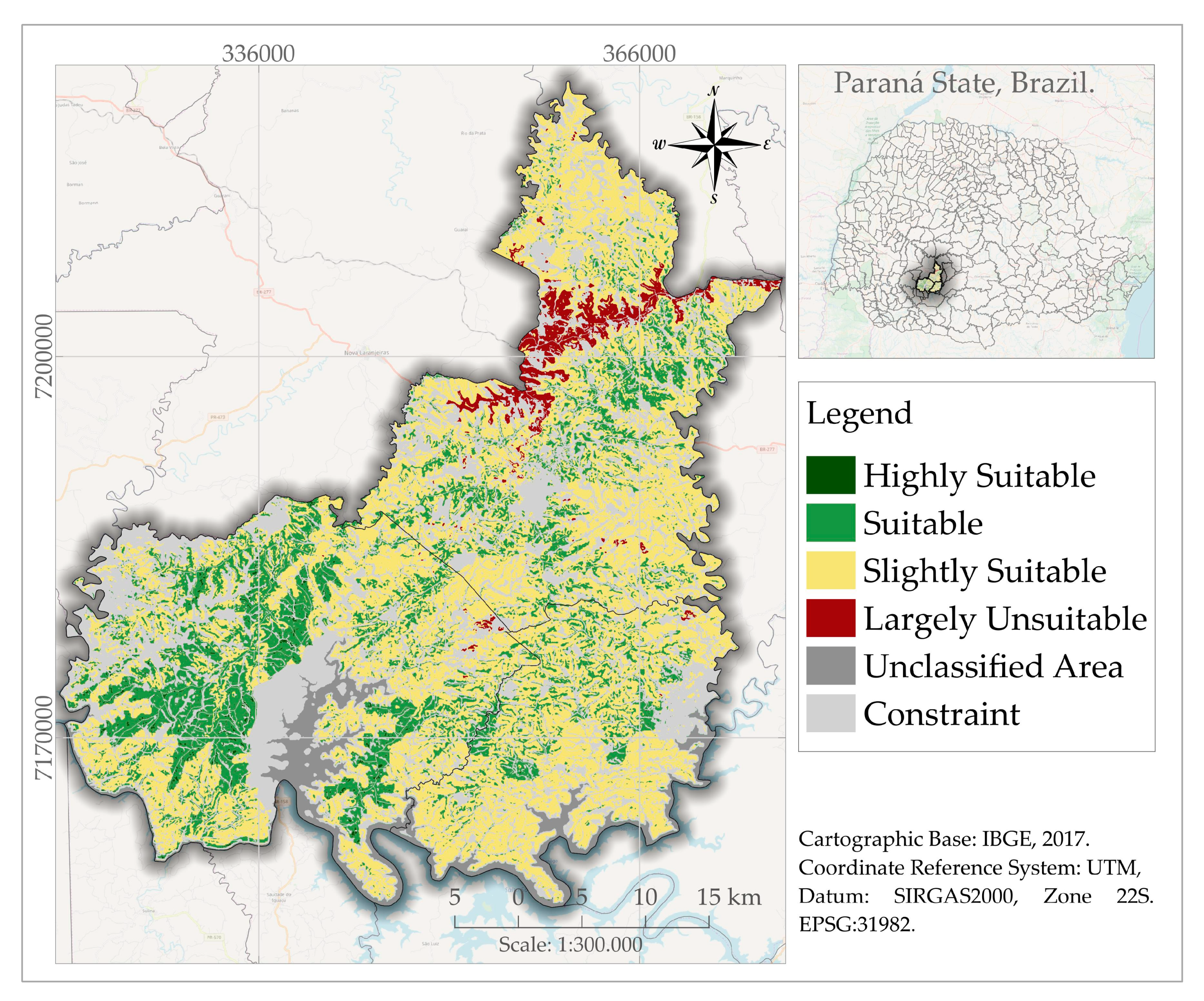
Hossain and Lin [52] argue that land should be divided into zones based on aquaculture suitability. Along a similar vein, this study created four categories to describe sites in the study area (highly suitable, suitable, slightly suitable, and largely unsuitable) in order to provide information on sites with potential for successful fish farming. The fish farming suitability map (Figure 6) was generated by overlaying maps of the four parameters (slope, altitude, soil type, and land use and occupation) using the AHP technique and GIS tools; areas with constraints (legal or otherwise) were removed from the model, as were non-classified areas. At the end of this process, it was estimated that 869.38 ha (0.49%) of the study area is highly suitable and that 32,401.41 ha (18.22%) is suitable for fish farming in ground-excavated ponds. This study therefore found that this region possesses a total of 33,270.79 ha (18.71% of its area) that is suitable for fish farming in ground-excavated ponds.

5. Conclusions

This study considered soil type, slope, altitude, and soil use and occupation in the identification and analysis of the most suitable sites for fish farming in ground-excavated ponds in three cities located in the central-southern region of Paraná State, Brazil.

Data processing in GIS and the use of a multi-criteria analysis allowed for the integration of variables and the establishment of relative weights between them; this combination of tools was found to be an adequate method for classifying areas as more or less suitable for fish farming in the study area.

When AHP analysis is combined with GIS to classify a given region for fish farming or other activities, the criteria and sub-criteria should be ranked by priority, as was done in this study. This ranking provides the classification levels of the priorities in a given interval (weights) which, after adding up all of the possible alternatives, will determine a manageable scale of priorities (Table 9) that can help to better combine the attributes for more accurate definitions of suitable sites.

The analysis of this region found that 18.71% of its area is appropriate for investment in fish farming; other areas may be used, though they exhibit varying degrees of limitations. The application of this method was found to be effective, and the results produced herein suggest that this method can be used by managers and entrepreneurs alike to increase the reliability of their attempts to identify the suitability of a given area for a given activity.