
Interpolation of Instantaneous Air Temperature Using Geographical and MODIS Derived Variables with Machine Learning Techniques


Abstract
1. Introduction
- Vertical lapse methods [4] use height as the main variable to explain temperature spatial distributions. The vertical lapse rate is evaluated from the sampling data and then applied to the whole study area. A more sophisticated approach uses daily atmospheric profiles provided by the Moderate Resolution Imaging Spectroradiometer (MODIS) product MOD07_L2 to locally estimate the adiabatic lapse rate [6]. The main drawback of this approach is the coarse spatial resolution (5 km) of those products.
- Multiple regression models using LST and other variables such as NDVI, solar zenith angle, solar radiation, altitude, julian day, distance to the coast, normalised difference water index (MNDWI) or albedo as predictors [8,9,10,11,12,13,14,15]. The algorithms used range from multiple linear regression [5,10,11,16] to more sophisticated machine learning algorithms, such as neural networks [9] or Random Forest (RF) [14].
- Geostatistical techniques (kriging) [17,18] estimate Ta as a weighting average of the sampling points with the weighting coefficients obtained after a statistical analysis of the spatial variability of the variable (semivariogram functions).The main drawbacks of such interpolation methods are that they do not use covariates and that they may be sensitive to a clustered distribution of weather stations [19].
- Methods based on the surface energy balance such as ADEBAT [4,13]. The objective is to estimate Ta using a more physical approach. It has two main drawbacks: several variables that can only be measured in weather stations are needed and, as the Bowen ratio (the ratio between the sensible heat flux and the latent heat flux) is one of them, it is necessary to know the latent heat flux (LE) to use ADEBAT. However, Ta is usually, as in this case, estimated in order to estimate LE from it, so the use of a surface energy balance is not suitable.
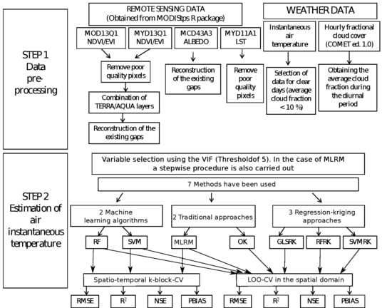
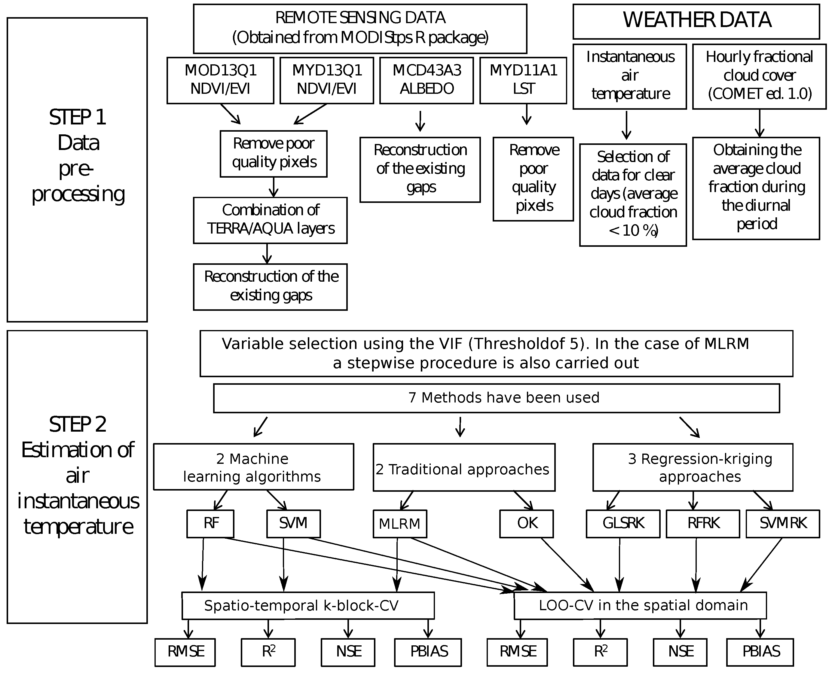
2. Methodology
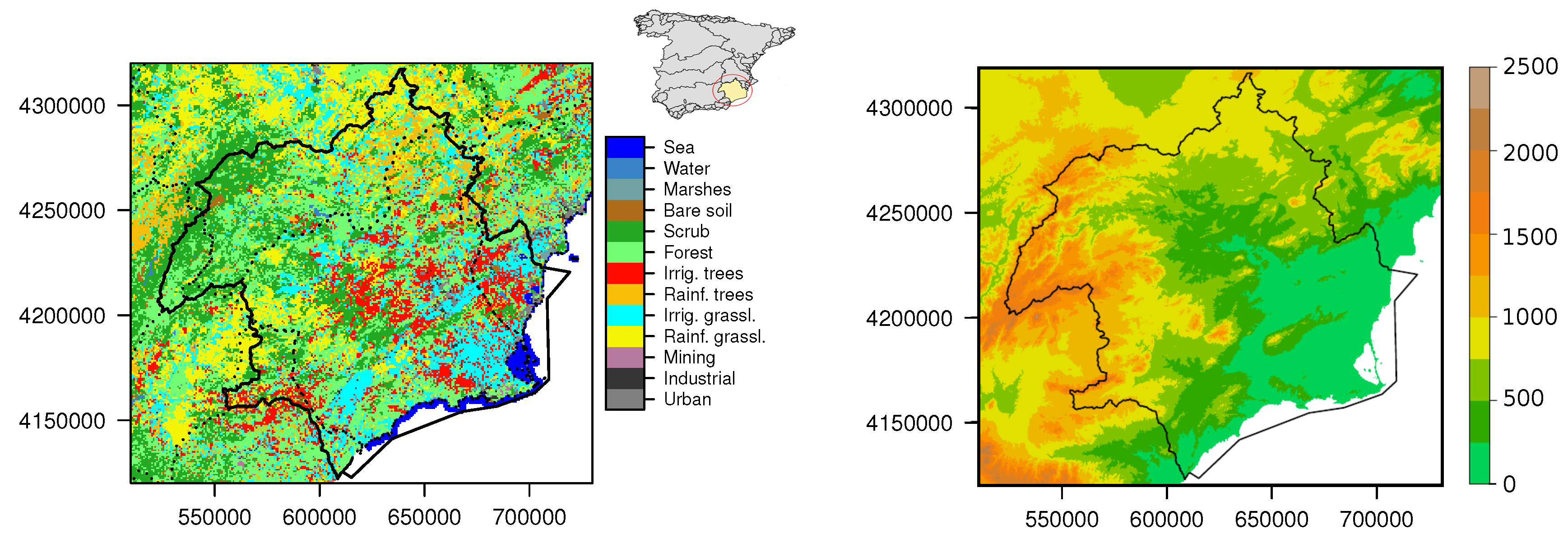
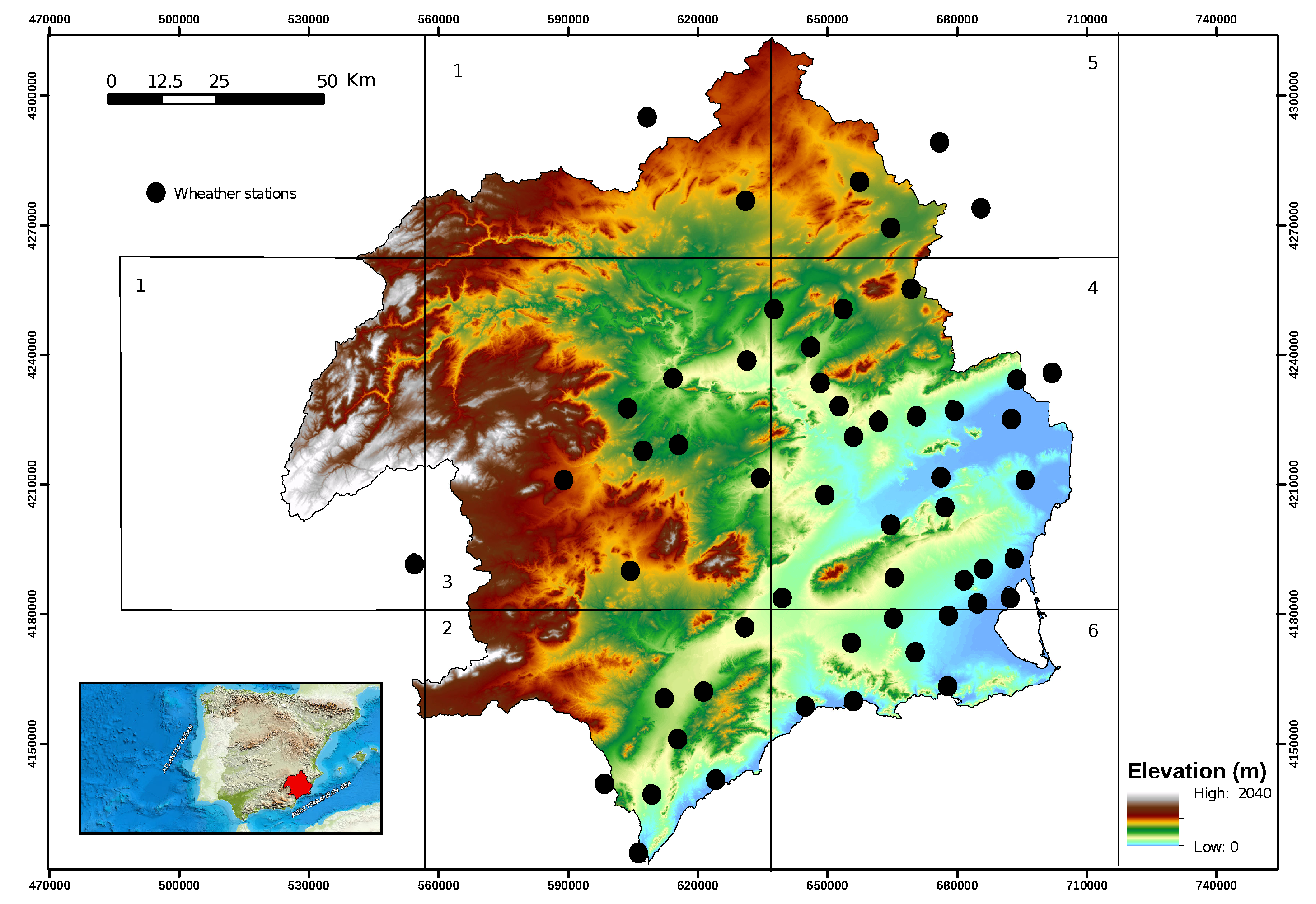
2.1. Study Area
2.2. Data Set
2.2.1. Weather Data
2.2.2. Remote Sensing Data
2.2.3. Geographical Variables
2.3. Estimation Methods
2.3.1. Multiple Linear Regression
2.3.2. Support Vector Machines
2.3.3. Random Forest
2.3.4. Ordinary Kriging
2.3.5. Regression-Kriging
2.3.6. Validation
3. Results
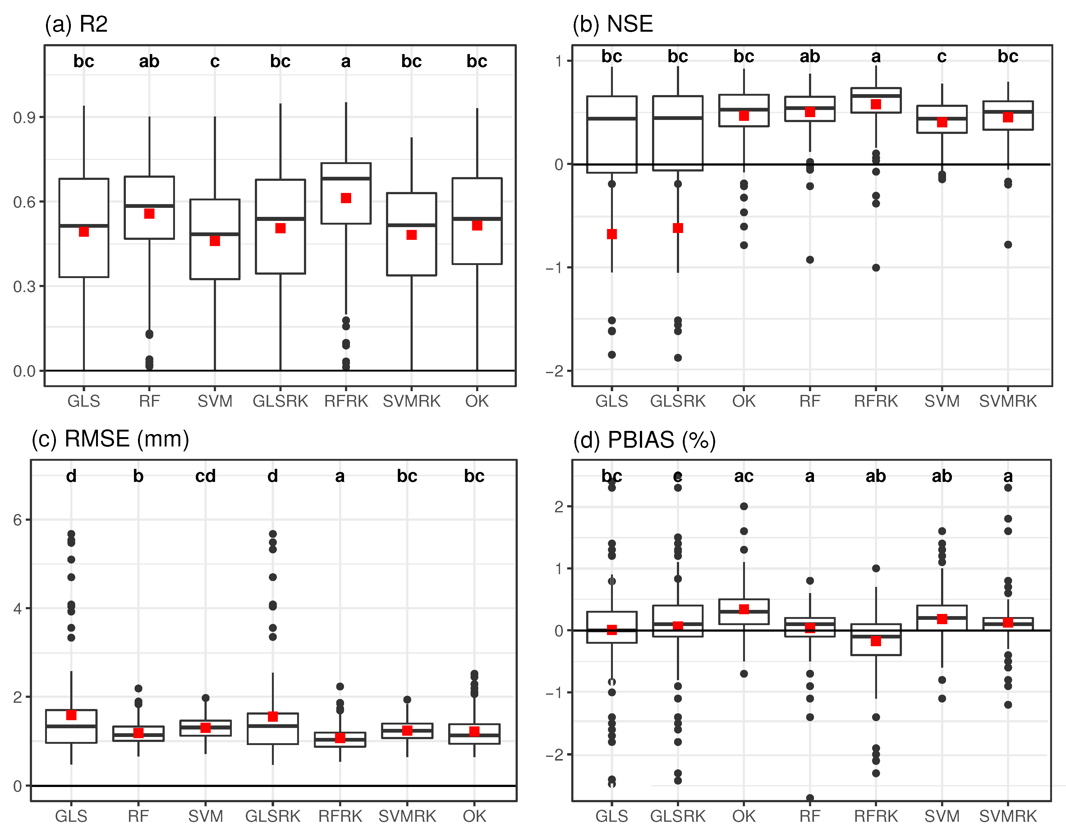
3.1. Leave-One-Out Cross-Validation in the Spatial Domain
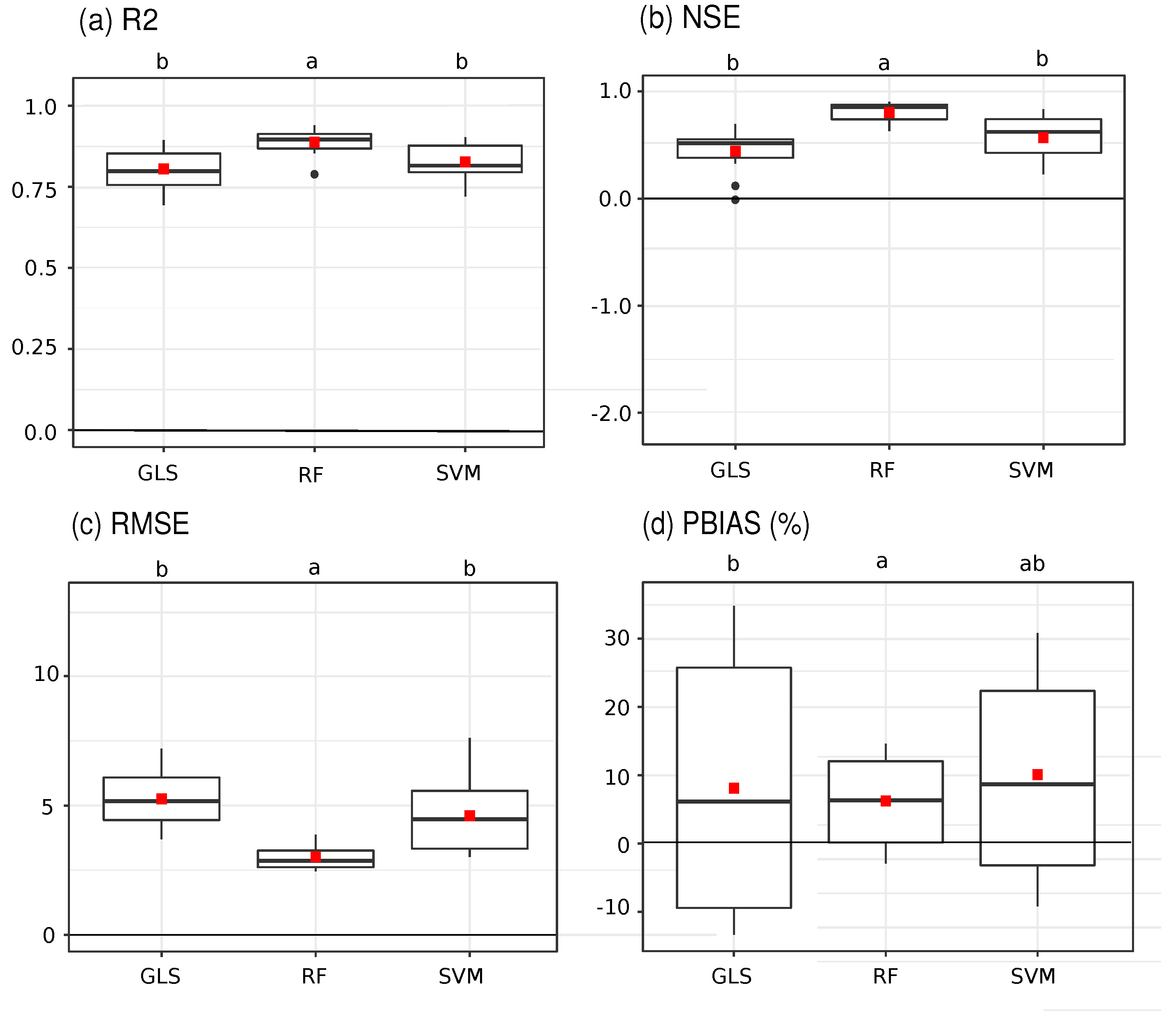
3.2. K-block Cross-Validation
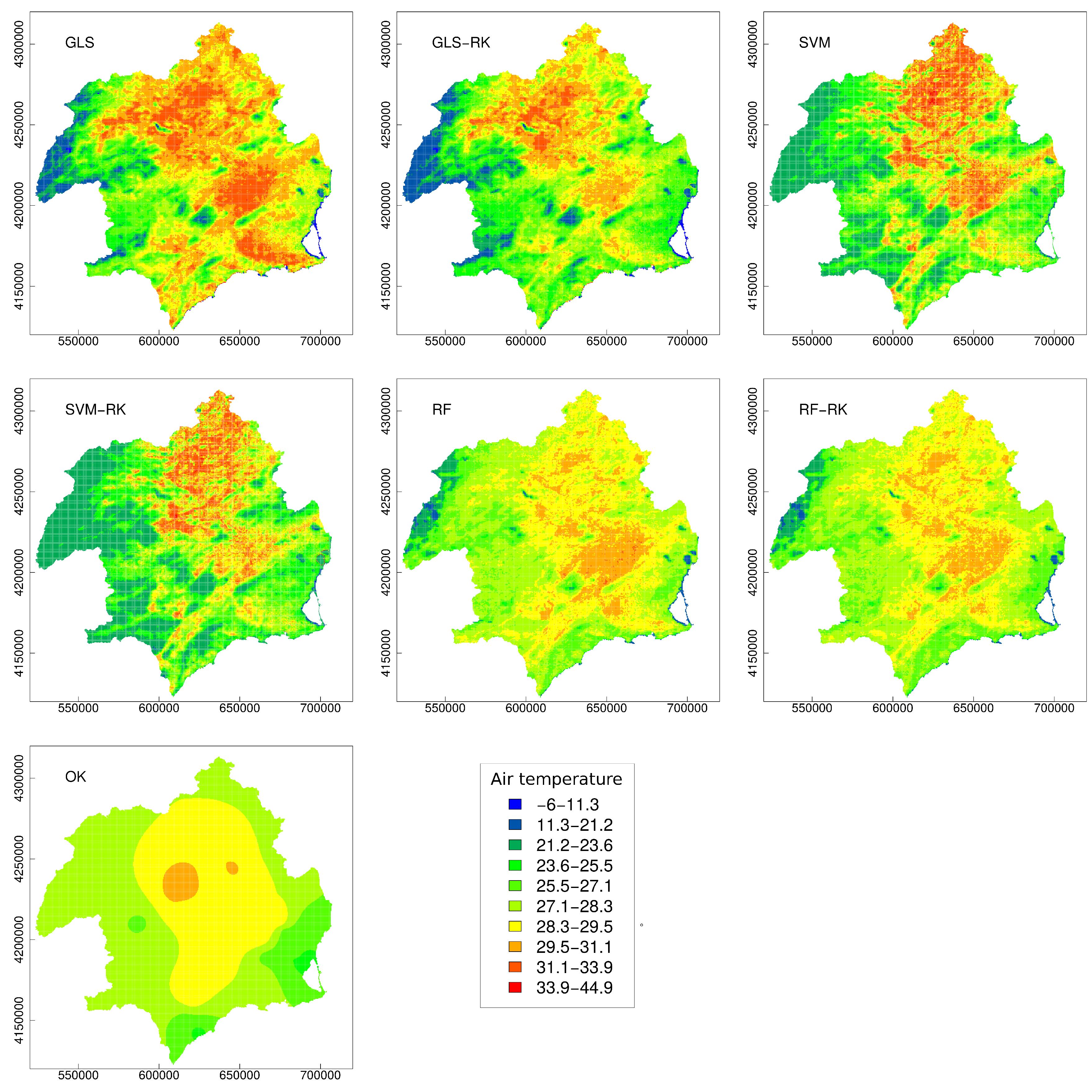
3.3. Final Prediction
4. Discussion
5. Conclusions
Author Contributions
Funding
Conflicts of Interest
Abbreviations
| DEM | Digital Elevation Model |
| EVI | Enhanced Vegetation Index |
| GLS | Generalised Least Squares |
| LST | Land Surface Temperature |
| MLRM | Multiple Linear Regression Model |
| MODIS | Moderate Resolution Imaging Spectroradiometer |
| OK | Ordinary Kriging |
| OLS | Ordinary Least Squares |
| RF | Random Forest |
| RK | Regression-kriging |
| SVM | Support Vector Machine |
| TVX | Temperature-Vegetation Index |
| TWI | Topographic Wetness Index |
| VIF | Variance Inflation Factor |
References
- Liu, S.; Su, H.; Zhang, R.; Tian, J.; Wang, W. Estimating the Surface Air Temperature by Remote Sensing in Northwest China Using an Improved Advection-Energy Balance for Air Temperature Model. Adv. Meteorol. 2016, 11. [Google Scholar] [CrossRef]
- Prihodko, L.; Goward, S.N. Estimation of air temperature from remotely sensed surface observations. Remote Sens. Environ. 1997, 60, 335–346. [Google Scholar] [CrossRef]
- Nieto, H.; Sandholt, I.; Aguado, I.; Chuvieco, E.; Stisen, E. Air temperature estimation with MSG-SEVIRI data: Calibration and validation of the TVX algorithm for the Iberian Peninsula. Remote Sens. Environ. 2011, 115, 107–116. [Google Scholar] [CrossRef]
- Zhang, R.; Rong, Y.; Tian, J.; Su, H.; Li, Z.L.; Liu, S. A Remote Sensing Method for Estimating Surface Air Temperature and Surface Vapor Pressure on a Regional Scale. Remote Sens. 2015, 7, 6005–6025. [Google Scholar] [CrossRef]
- Liu, S.; Su, H.; TIAN, J.; Zhang, R.; Wang, W.; Wu, Y. Evaluating Four Remote Sensing Methods for Estimating Surface Air Temperature on a Regional Scale. J. Appl. Meteorol. Climatol. 2017, 56, 803–814. [Google Scholar] [CrossRef]
- Zhu, W.; Lu, A.; Jia, S.; Yan, J.; Mahmood, R. Retrievals of all-weather daytime air temperature from MODIS products. Remote Sens. Environ. 2017, 189, 152–163. [Google Scholar] [CrossRef]
- Vogt, J.; Viau, A.; Paquet, F. Mapping regional air temperature fields using satellite-derived surface skin temperatures. Int. J. Climatol. 1997, 17, 1559–1579. [Google Scholar] [CrossRef]
- Cresswell, M.; Morse, A.; Thomson, M.; Connor, S. Estimating surface air temperatures, from Meteosat land surface temperatures, using an empirical solar zenith angle model. Int. J. Remote Sens. 1999, 20, 1125–1132. [Google Scholar] [CrossRef]
- Jang, J.; Viau, A.; Anctil, F. Neural network estimation of air temperatures from AVHRR data. Int. J. Remote Sens. 2004, 25, 4541–4554. [Google Scholar] [CrossRef]
- Lin, S.; Moore, N.; Messina, J.; DeVisser, M.; Wu, J. Evaluation of estimating daily maximum and minimum air temperature with MODIS data in east Africa. Int. J. Appl. Earth Obs. Geoinf. 2012, 18, 128–140. [Google Scholar] [CrossRef]
- Benali, A.; Carvalho, A.; Nunes, J.; Carvalhais, N.; Santos, A. Estimating Air Surface Temperature in Portugal Using MODIS LST Data. Remote Sens. Environ. 2012, 124, 108–121. [Google Scholar] [CrossRef]
- Kim, D.; Han, K. Remotely Sensed Retrieval of Midday Air Temperature Considering Atmospheric and Surface Moisture Conditions. Int. J. Remote Sens. 2013, 34, 247–263. [Google Scholar] [CrossRef]
- Zakšek, K.; Schroedter-Homscheidt, M. Parameterization of air temperature in high temporal and spatial resolution from a combination of the SEVIRI and MODIS instruments. ISPRS J. Photogramm. Remote Sens. 2009, 64, 414–421. [Google Scholar] [CrossRef]
- Xu, Y.; Knudby, A.; Ho, H.C. Estimating daily maximum air temperature from MODIS in British Columbia, Canada. Int. J. Remote Sens. 2014, 35, 8108–8121. [Google Scholar] [CrossRef]
- Cristóbal, J.; Ninyerola, M.; Pons, X. Modeling air temperature through a combination of remote sensing and GIS data. J. Geophys. Res. 2008, 113, D13106. [Google Scholar] [CrossRef]
- Fu, G.; Shen, Z.; Zhang, X.; Shi, P.; Zhang, Y.; Wu, J. Estimating air temperature of an alpine meadow on the Northern Tibetan Plateau using MODIS land surface temperature. Acta Ecol. Sin. 2011, 21, 8–13. [Google Scholar] [CrossRef]
- Vancutsem, C.; Ceccato, P.; Dinku, T.; Connor, S. Evaluation of MODIS Land Surface Temperature Data to Estimate Air Temperature in Different Ecosystems over Africa. Remote Sens. Environ. 2010, 114, 449–465. [Google Scholar] [CrossRef]
- Kloog, I.; Nordio, F.; Coull, B.; Schwartz, J. Predicting Spatiotemporal Mean Air Temperature Using MODIS Satellite Surface Temperature Measurements across the Northeastern USA. Remote Sens. Environ. 2014, 150, 132–139. [Google Scholar] [CrossRef]
- Yang, Y.Z.; Cai, W.H.; Yang, J. Evaluation of MODIS Land Surface Temperature Data to Estimate Near-Surface Air Temperature in Northeast China. Remote Sens. 2017, 9, 410. [Google Scholar] [CrossRef]
- Nemani, R.R.; Running, S.W. Estimation of regional surface resistance to evapotranspiration from NDVI and thermal-IR AVHRR data. J. Appl. Meteorol. 1989, 28, 276–284. [Google Scholar] [CrossRef]
- Goward, S.N.; Waring, R.; Dye, D.; Yang, J. Ecological remote sensing at OTTER: Satellite macroscale observations. Ecol. Appl. 1994, 4, 322–343. [Google Scholar] [CrossRef]
- Czajkowski, K.; Mulhern, T.; Goward, S.; Cihlar, J.; Dubayah, R.; Prince, S. Biospheric environmental monitoring at BOREAS with AVHRR observations. J. Geophys. Res. 1997, 102, 651–662. [Google Scholar] [CrossRef]
- Tao, J.; Zhang, Y.; Zhu, J.; Jiang, Y.; Zhang, X.; Zhang, T.; Xi, Y. Elevation-Dependent Temperature Change in the Qinghai-Xizang Plateau Grassland During the Past Decade. Theor. Appl. Climatol. 2013, 117, 61–71. [Google Scholar] [CrossRef]
- Jin, M.; Dickinson, R. Interpolation of surface radiative temperature measured from polar orbiting satellites to a diurnal cycle: 1. without clouds. J. Geophys. Res. Atmos. 1999, 104, 2105–2116. [Google Scholar] [CrossRef]
- Sun, D.; Pinker, R.; Kafatos, M. Diurnal temperature range over the United States: A satellite view. Geophys. Res. Lett. 2006, 33. [Google Scholar] [CrossRef]
- Gholamnia, M.; Alavipanah, S.K.; Boloorani, A.D.; Hamzeh, S.; Kiavarz, M. Diurnal Air Temperature Modeling Based on the Land Surface Temperature. Remote Sens. 2017, 9, 915. [Google Scholar] [CrossRef]
- Golkar, F.; Sabziparvar, A.A.; Khanbilvardi, R.; Nazemosadat, M.J.; Zand-Parsa, S.; Rezaei, Y. Estimation of instantaneous air temperature using remote sensing data. Int. J. Remote Sens. 2018, 39, 258–275. [Google Scholar] [CrossRef]
- Mira, M.; Ninyerola, M.; Batalla, M.; Pesquer, L.; Pons, X. Improving Mean Minimum and Maximum Month-to-Month Air Temperature Surfaces Using Satellite-Derived Land Surface Temperature. Remote Sens. 2017, 9, 1313. [Google Scholar] [CrossRef]
- Hooker, J.; Duveiller, G.; Cescatti, A. A global dataset of air temperature derived from satellite remote sensing and weather stations. Sci. Data 2018, 5, 1–11. [Google Scholar] [CrossRef]
- Neteler, M.; Mitasova, H. Open Source GIS: A GRASS GIS Approach; Springer Science & Business Media: Boston, MA, USA, 2013; Volume 689. [Google Scholar]
- R Core Team. R: A Language and Environment for Statistical Computing; R Foundation for Statistical Computing: Vienna, Austria, 2018. [Google Scholar]
- Confederación Hidrográfica del Segura. Plan Hidrológico de la demarcación hidrográfica del Segura. Ciclo de planificación hidrológica 2015–2021; Technical Report; Ministerio para la Transición Ecológica: Madrid, Spain, 2015.
- Conesa García, C.; Alonso Sarria, F. El clima de la Región de Murcia; Editum: Murcia, Spain, 2006; pp. 95–128. [Google Scholar]
- Sørensen, R.; Zinko, U.; Seibert, J. On the calculation of the topographic wetness index: Evaluation of different methods based on field observations. Hydrol. Earth Syst. Sci. 2006, 10, 101–112. [Google Scholar] [CrossRef]
- Hofierka, J.; Suri, M. The solar radiation model for Open source GIS: implementation and applications. In Proceedings of the International GRASS Users Conference, Trento, Italy, 11–13 September 2002. [Google Scholar]
- Gasch, C.; Hengl, T.; Gräler, B.; Meyer, H.; Magney, T.; Brown, D. Spatio-temporal interpolation of soil water, temperature, and electrical conductivity in 3D + T: The Cook Agronomy Farm data set. Spat. Stat. 2015, 14, 70–90. [Google Scholar] [CrossRef]
- Beven, K. Runoff production and flood frequency in catchments of order n: An alternative approach. In Scale Problems in Hydrology; Gupta, V.K., Rodriguez-Iturbe, I., Wood, E., Eds.; Reidel: Dordrecht, The Netherlands, 1986; pp. 107–131. [Google Scholar]
- Hengl, T.; Reuter, H.I. Geomorphometry: Concepts, Software, Applications; Elsevier: Amsterdam, The Netherlands, 2009; p. 796. [Google Scholar]
- Busetto, L.; Ranghetti, L. MODIStsp: An R package for automatic preprocessing of MODIS Land Products time series. Comput. Geosci. 2016, 97, 40–48. [Google Scholar] [CrossRef]
- Priyadarshi, N.; Chowdary, V.; Srivastava, Y.; Das, I.C.; Jha, C.S. Reconstruction of time series MODIS EVI data using de-noising algorithms. Geocarto Int. 2017, 33, 1095–1113. [Google Scholar] [CrossRef]
- Huete, A.; Justice, C.; Van Leeuwen, W. MODIS vegetation index (MOD13). Algorithm Theor. Basis Doc. 1999, 3, 213. [Google Scholar]
- Gu, J.; Li, X.; Huang, C.; Okin, G.S. A simplified data assimilation method for reconstructing time-series MODIS NDVI data. Adv. Space Res. 2009, 44, 501–509. [Google Scholar] [CrossRef]
- Metz, M.; Andreo, V.; Neteler, M. A New Fully Gap-Free Time Series of Land Surface Temperature from MODIS LST Data. Remote Sens. 2017, 9, 1333. [Google Scholar] [CrossRef]
- Stöckli, R.; Duguay–Tetzlaff, A.; Bojanowski, J.; Hollmann, R.; Fuchs, P.; Werscheck, M. CM SAF ClOud Fractional Cover Dataset from METeosat First and Second Generation—Edition 1 (COMET Ed. 1); Satellite Application Facility on Climate Monitoring: Darmstadt, Germany, 2017. [Google Scholar] [CrossRef]
- Pinheiro, J.; Bates, D.; DebRoy, S.; Sarkar, D.; R Core Team. Nlme: Linear and Nonlinear Mixed Effects Models; Technical Report; R Foundation for Statistical Computing: Vienna, Austria, 2018. [Google Scholar]
- Zuur, A.; Ieno, E.; Walker, N.; Saveliev, A.; Smith, G. Mixed Effects Models and Extensions in Ecology with R; Springer: Berlin/Heidelberg, Germany, 2009; p. 549. [Google Scholar]
- Cortes, C.; Vapnik, V. Support-Vector Networks. Mach. Learn. 1995, 20, 273–297. [Google Scholar]
- Kuhn, M.; Johnson, K. Applied Predictive Modeling; Springer: Berlin/Heidelberg, Germany, 2013. [Google Scholar]
- Murphy, K. Machine Learning. A Propbabilistic Approach; The MIT Press: Cambridge, MA, USA, 2012. [Google Scholar]
- Radhika, Y.; Shashi, M. Atmospheric Temperature Prediction using Support Vector Machines. Int. J. Comput. Theory Eng. 2009, 1, 1793–8201. [Google Scholar] [CrossRef]
- Balabin, R.; Lomakina, E. Support vector machine regression (LS-SVM)—An alternative to artificial neural networks (ANNs) for the analysis of quantum chemistry data? Phys. Chem. Chem. Phys. 2011, 13, 11710–11718. [Google Scholar] [CrossRef]
- Nagendra, K.V.; Jahnavi, Y.; Haritha, N. A Survey on Support Vector Machines and Artificial Neural Network in Rainfall Forecasting. Int. J. Future Revolut. Comput. Sci. Commun. Eng. 2017, 3, 20–24. [Google Scholar]
- Meyer, D.; Dimitriadou, E.; Hornik, K.; Weingessel, A.; Leisch, F. e1071: Misc Functions of the Department of Statistics, Probability Theory Group (Formerly: E1071), TU Wien; Technical Report; R Foundation for Statistical Computing: Vienna, Austria, 2018. [Google Scholar]
- Breiman, L. Random Forests. Mach. Learn. 2001, 45, 5–32. [Google Scholar] [CrossRef]
- Wright, M.N.; Ziegler, A. ranger: A Fast Implementation of Random Forests for High Dimensional Data in C++ and R. J. Stat. Softw. 2017, 77, 1–17. [Google Scholar] [CrossRef]
- Liaw, A.; Wiener, M. Classification and Regression by randomForest. R News 2002, 2, 18–22. [Google Scholar]
- Cánovas-García, F.; Alonso-Sarria, F. Optimal Combination of Classification Algorithms and Feature Ranking Methods for Object-Based Classification of Submeter Resolution Z/I-Imaging DMC Imagery. Remote Sens. 2015, 74, 4651–4677. [Google Scholar] [CrossRef]
- Burrough, P.; McDonnell, R.; Lloyd, C. Principles of Geographical Information Systems; Oxford University Press: Oxford, UK, 2015. [Google Scholar]
- Hiemstra, P.; Pebesma, E.; Twenhöfel, C.; Heuvelink, G. Real-time automatic interpolation of ambient gamma dose rates from the Dutch Radioactivity Monitoring Network. Comput. Geosci. 2008, 35, 1711–1721. [Google Scholar] [CrossRef]
- Cressie, N. Statistics for Spatial Data (Revised Ed); Wiley: Hoboken, NJ, USA, 1993. [Google Scholar]
- Hengl, T.; Heuvelink, G.B.; Rossiter, D.G. About regression-kriging: From equations to case studies. Comput. Geosci. 2007, 33, 1301–1315. [Google Scholar] [CrossRef]
- Odeh, I.; McBratney, A.; Chittleborough, D. Further results on prediction of soil properties from terrain attributes: Heterotopic cokriging and regression-kriging. Geoderma 1995, 67, 215–226. [Google Scholar] [CrossRef]
- Hengl, T.; Heuvelink, G.B.; Stein, A. A generic framework for spatial prediction of soil variables based on regression-kriging. Geoderma 2004, 120, 75–93. [Google Scholar] [CrossRef]
- Roberts, D.; Bahn, V.; Ciuti, S.; Boyce, M.; Elith, J.; Guillera-Arroita, G.; Hauenstein, S.; Lahoz-Monfort, J.; Schröder, B.; Thuiller, W.; et al. Cross-validation strategies for data with temporal, spatial, hierarchical, or phylogenetic structure. Ecography 2017, 40, 913–929. [Google Scholar] [CrossRef]
- Meyer, H.; Reudenbach, C.; Hengl, T.; Katurji, M.; Nauss, T. Improving performance of spatio-temporal machine learning models using forward feature selection and target-oriented validation. Environ. Model. Softw. 2018, 101, 1–9. [Google Scholar] [CrossRef]
- Trachsel, M.; Telford, R. Technical note: Estimating unbiased transfer-function performances in spatially structured environments. Clim. Past 2016, 12, 1215–1223. [Google Scholar] [CrossRef]
- Valavi, R.; Elith, J.; Lahoz-Monfort, J.; Guillera-Arroita, G. blockcv: An r package for generating spatially or environmentally separated folds for k-fold cross-validation of species distribution models. Methods Ecol. Evol. 2019, 10, 225–232. [Google Scholar] [CrossRef]
- Bennett, N.D.; Croke, B.F.; Guariso, G.; Guillaume, J.H.; Hamilton, S.H.; Jakeman, A.J.; Marsili-Libelli, S.; Newham, L.T.; Norton, J.P.; Perrin, C.; et al. Characterising performance of environmental models. Environ. Model. Softw. 2013, 40, 1–20. [Google Scholar] [CrossRef]
- Legates, D.R.; McCabe, G.J. Evaluating the use of “goodness-of-fit” Measures in hydrologic and hydroclimatic model validation. Water Resour. Res. 1999, 35, 233–241. [Google Scholar] [CrossRef]
- Long, J.; Ervin, L. Using Heteroscedasticity Consistent Standard Errors in the Linear Regression Model. Am. Stat. 2000, 54, 217–224. [Google Scholar]
- O’Brien, R.M. A caution regarding rules of thumb for variance inflation factors. Quality & Quantity 2007, 45, 673–690. [Google Scholar] [CrossRef]
- Kutner, M.H.; Nachtsheim, C.; Neter, J. Applied Linear Regression Models; McGraw-Hill/Irwin: New York, NY, USA, 2004. [Google Scholar]
- Juutilainen, I.; Röning, J.; Laurinen, P. A study on the differences in the interpolation capabilities of models. In Proceedings of the 2005 IEEE Midnight-Summer Workshop on Soft Computing in Industrial Applications, 2005 SMCia/05, Espoo, Finland, 28–30 June 2005; pp. 202–207. [Google Scholar] [CrossRef]
- Ishwaran, H.; Kogalur, U. Fast Unified Random Forests for Survival, Regression, and Classification (RF-SRC), R package version 2.9.0; R Foundation for Statistical Computing: Vienna, Austria, 2019. [Google Scholar]
- Bisht, G.; Bras, R.L. Estimation of net radiation from the MODIS data under all sky conditions: Southern Great Plains case study. Remote. Sens. Environ. 2010, 114, 1522–1534. [Google Scholar] [CrossRef]
- Xiong, Y.J.; Zhao, S.H.; Tian, F.; Qiu, G.Y. An evapotranspiration product for arid regions based on the three-temperature model and thermal remote sensing. J. Hydrol. 2015, 530, 392–404. [Google Scholar] [CrossRef]
- Zhu, W.; Jia, S.; Lv, A. A Universal Ts-VI Triangle Method for the Continuous Retrieval of Evaporative Fraction From MODIS Products. J. Geophys. Res. Atmos. 2017, 122, 10–206. [Google Scholar] [CrossRef]
Sample Availability: Samples of the compounds are available from the authors. |


| Sensor | Platform | Layer | Name | Spatial Res. (km) | Temporal Res. (days) |
|---|---|---|---|---|---|
| MODIS | Aqua | , | MYD11A1 | 1 | 1 |
| MODIS | Terra + Aqua | Albedo, | MCD43A3 | 0.5 | 1 (16 days average) |
| MODIS | Terra | EVI | MOD13Q1 | 0.25 | 16 |
| MODIS | Aqua | EVI | MYD13Q1 | 0.25 | 16 |
| GLS | RF | SVM | GLSRK | RFRK | SVMRK | OK | |
|---|---|---|---|---|---|---|---|
| R2 | 0.493 ± 0.024 | 0.558 ± 0.019 | 0.460 ± 0.018 | 0.506 ± 0.024 | 0.612 ± 0.019 | 0.482 ± 0.018 | 0.515 ± 0.021 |
| NSE | −0.679 ± 0.43 | 0.504 ± 0.022 | 0.405 ± 0.019 | −0.620 ± 0.423 | 0.578 ± 0.025 | 0.452 ± 0.021 | 0.468 ± 0.029 |
| RMSE | 1.587 ± 0.097 | 1.181 ± 0.025 | 1.301 ± 0.025 | 1.550 ± 0.096 | 1.068 ± 0.027 | 1.236 ± 0.023 | 1.214 ± 0.036 |
| PBIAS | 0.009 ± 0.144 | 0.036 ± 0.038 | 0.184 ± 0.037 | 0.060 ± 0.151 | −0.172 ± 0.046 | 0.125 ± 0.038 | 0.340 ± 0.033 |
| GLS | RF | SVM | |
|---|---|---|---|
| R2 | 0.805 ± 0.039 | 0.888 ± 0.026 | 0.827 ± 0.036 |
| NSE | 0.444 ± 0.135 | 0.805 ± 0.064 | 0.571 ± 0.135 |
| RMSE | 5.251 ± 0.693 | 3.009 ± 0.325 | 4.606 ± 0.968 |
| PBIAS | 8.142 ± 12.249 | 6.258 ± 4.013 | 10.092 ± 9.528 |
© 2019 by the authors. Licensee MDPI, Basel, Switzerland. This article is an open access article distributed under the terms and conditions of the Creative Commons Attribution (CC BY) license (http://creativecommons.org/licenses/by/4.0/).
Share and Cite
Ruiz-Álvarez, M.; Alonso-Sarria, F.; Gomariz-Castillo, F. Interpolation of Instantaneous Air Temperature Using Geographical and MODIS Derived Variables with Machine Learning Techniques. ISPRS Int. J. Geo-Inf. 2019, 8, 382. https://doi.org/10.3390/ijgi8090382
Ruiz-Álvarez M, Alonso-Sarria F, Gomariz-Castillo F. Interpolation of Instantaneous Air Temperature Using Geographical and MODIS Derived Variables with Machine Learning Techniques. ISPRS International Journal of Geo-Information. 2019; 8(9):382. https://doi.org/10.3390/ijgi8090382
Chicago/Turabian StyleRuiz-Álvarez, Marcos, Francisco Alonso-Sarria, and Francisco Gomariz-Castillo. 2019. "Interpolation of Instantaneous Air Temperature Using Geographical and MODIS Derived Variables with Machine Learning Techniques" ISPRS International Journal of Geo-Information 8, no. 9: 382. https://doi.org/10.3390/ijgi8090382
APA StyleRuiz-Álvarez, M., Alonso-Sarria, F., & Gomariz-Castillo, F. (2019). Interpolation of Instantaneous Air Temperature Using Geographical and MODIS Derived Variables with Machine Learning Techniques. ISPRS International Journal of Geo-Information, 8(9), 382. https://doi.org/10.3390/ijgi8090382