Anomalous Urban Mobility Pattern Detection Based on GPS Trajectories and POI Data

Abstract

Anomalous urban mobility pattern refers to abnormal human mobility flow in a city. Anomalous urban mobility pattern detection is important in the study of urban mobility. In this paper, a framework is proposed to identify anomalous urban mobility patterns based on taxi GPS trajectories and Point of Interest (POI) data. In the framework, functional regions are first generated based on the distribution of POIs by the DBSCAN clustering algorithm. A Weighted Term Frequency-Inverse Document Frequency (WTF-IDF) method is proposed to identify function values in each region. Then, the Origin-Destination (OD) of trips between functional regions is extracted from GPS trajectories to detect anomalous urban mobility patterns. Mobility vectors are established for each time interval based on the OD of trips and are classified into clusters by the mean shift algorithm. Abnormal urban mobility patterns are identified by processing the mobility vectors. A case study in the city of Wuhan, China, is conducted; the experimental results show that the proposed method can effectively identify daily and hourly anomalous urban mobility patterns.

1. Introduction

Urban mobility research studies the mobile flow of residents in urban areas [1,2,3,4,5,6]. The majority of human movement flows behave with a certain regularity, which are called normal urban mobility patterns. Anomalous urban mobility patterns are those that do not conform to normal regularity and that usually occur during special occasions, such as concerts or sport events. It is very informative for administrators to discover and understand anomalous urban mobility patterns. For instance, pattern detection can determine if emergencies are occurring in a city. It may help decision-makers take timely action to mitigate potential traffic congestion resulting from the anomalous mobility.

In the last few decades, with the development of information technology, mobile devices equipped with global positioning system (GPS) receivers are widely used, which makes a large amount of GPS data recording human movement available to study mobility [7,8]. Points of interest (POI) data in urban areas are also collected and provided by many map producers, which could help better understand the functional structure of urban areas and the purpose of human mobility [9,10].

Extracting human movement patterns and determining anomalous movement patterns are major challenges in data mining of massive trajectory datasets. The first challenge is how to identify functional regions effectively. The development of a city may deviate from the planning of the government [11,12,13]. Thus, the study of functional regions is important in understanding the functional structure of a city and is helpful in making adjustments in urban planning if necessary. Many existing methods to identify functional regions in urban areas are based on strong assumptions. Wang et al. [3] assumed that 500 m is the traditional walking distance of people’s travel activity; they separated a city into functional regions based on 1 km × 1 km grids. Yuan et al. [11] assumed that the basic units divided by major roads carry certain social-economic functions that can be used to represent functional regions. Nonetheless, these methods may split one integrated functional region into several smaller regions, which may be unreasonable. For example, university campuses separated by a major road should be considered as one functional region. More importantly, POI data, which provide important information about different types of functions within a region, are not fully considered in current functional region identification methods. Therefore, how to divide an urban area into functional regions based on POI data itself is a problem, as the spatial distributions of POIs are highly irregular.

In addition, it is challenging to describe the functions of a region based on POI data since every functional region contains multiple POIs providing different services. The conventional Term Frequency and Inverse Document Frequency technique (TF-IDF) are used to deal with the issue [11], but they underestimate the impact of feature POIs on a region’s function. Feature POIs are those that dominate the function of a region, although their frequencies may be very small, such as hospitals for a region of medical services and railway stations for a region of transportation. Therefore, an effective method to identify a region’s function by considering the significance of the feature POIs is worthy exploring.

The last challenge is how to detect anomalous urban mobility patterns effectively between functional regions. Previous studies [14,15,16] focused on whether anomalous mobility patterns exist in the urban area, but specific anomalous mobility patterns between functional regions were not identified. Moreover, anomalous urban mobility patterns may vary with temporal granularity, such as by hour or day. For example, some anomalous urban mobility patterns can be detected at a small temporal scale, while they would be inundated by other major urban mobility patterns at a larger temporal scale. Therefore, studying anomalous mobility patterns at different temporal scales is important.

In this paper, an effective framework to detect anomalous urban mobility patterns between functional regions at different temporal scales is proposed. Functional regions are first identified based on the spatial distribution of POIs. DBSCAN, a density-based clustering method, is used to aggregate POIs into regions.

An extension of the TF-IDF technique, called Weighted TF-IDF (WTF-IDF), is used to calculate the function values in each region based on POIs.

To identify anomalous urban mobility patterns, Origin-Destination (OD) of trips is extracted from taxi GPS trajectory data. Then, mobility vectors are established to represent the distribution of OD in different time intervals, and the mean shift clustering method is applied to group the mobility vectors into clusters. Next, each cluster is taken as a mobility pattern. The anomalous and normal mobility patterns are differentiated based on the frequency of mobility vectors.

Specifically, the contributions of the paper are summarized as follows:

• Functional regions are effectively identified based on POI data. DBSCAN, a density-based clustering algorithm, is applied to identify functional regions. The weighted TF-IDF technique, considering the significance of feature POIs, is proposed to calculate the function values of functional regions.
• Mobility vectors, extracted from OD trips, are proposed to record the information of human movement; the mean shift algorithm is used to aggregate the movements into different urban mobility patterns. Anomalous urban mobility patterns can be detected and differentiated from normal urban mobility patterns in urban areas. Additionally, this method can effectively detect anomalous mobility patterns at different temporal scales.
• A case study is conducted using taxi GPS trajectory and POI data in the city of Wuhan, China. The results show that the proposed method can effectively identify functional regions and interesting mobility patterns.

The sections of this paper are organized as follows: Section 2 introduces the related work of functional region identification and urban mobility patterns. Section 3 details the proposed method of functional region identification and anomalous mobility pattern mining. Section 4 describes a case study using an observed dataset from the city of Wuhan. Section 5 presents conclusions and the future work of this paper.

2. Related Work

In recent years, many studies have focused on urban computing, including functional region discovery and urban mobility detection.

2.1. Functional Region Discovery

Functional regions provide one or more services for residents in urban areas. Different methods have been proposed to extract functional regions and estimate the function distribution of the regions.

Some researchers used grids with a fixed size to partition urban areas into functional regions. For example, Wang et al. [3] divided a city into functional regions with grids. Other methods partition urban areas based on major roads. For example, Yuan et al. [11] first extracted the major roads from the road network, then segmented the whole urban area into smaller regions based on the extracted roads. Both methods partitioned a city into functional regions based on strong assumptions and did not consider the geo-spatial distribution of POIs in the functional regions. For example, if we use major roads to create functional regions, some POIs with the same function distribution on both sides of the road will be separated into two functional regions.

Many methods have been proposed to estimate function values of regions. Yuan et al. [12] applied the Latent Dirichlet Allocation (LDA) model to discover the topics of a region based on POI data. Gao et al. [17] developed a statistical framework to study functional regions and their semantic topics based on the co-occurrence patterns of POI types. They first used the K-means clustering method and Delaunay triangulation with spatial constraints to extract urban functional regions. Then, distinctive latent topics of the regions were identified by the LDA model based on POI type. Last, they showed that a region could support multiple functions with different probabilities; the regions with the same function could span multiple locations, which were geographically non-adjacent. Qi et al. [13] identified the functions of city regions with OD trips, which were extracted from a large taxi trajectory dataset. The OD patterns discovered can characterize the social functions of city regions. Train stations, scenic spots and entertainment districts were identified as the three typical functions. This research could help local governments learn city dynamics. Cao et al. [18] used the trajectory data from mobile phones and check-ins of social media to explore the distribution and dynamics of functional regions. First, individual trips were extracted from phone call data, which provided information about users’ daily mobility. Then, Weibo check-in data were used as prior knowledge to infer functional regions based on the activity-labelling model. Wang et al. [3] classified the urban area into three categories with non-negative matrix factorization, denoted as H1 grids, H2 grids, and H3 grids. The classification indicated that functional regions were correlated with OD flows. They allocated POIs of each category into grids, then identified spatial semantics of functional regions with the dominating POI category.

2.2. Urban Mobility Pattern Detection

Trajectory data have been widely used to study urban mobility patterns. Kaltenbrunner et al. [19] studied urban mobility patterns based on bicycle trajectory data in Barcelona, Spain. They detected spatial and temporal mobility patterns of bicycle flows in the city and applied these patterns to predict the number of available bikes at bike stations. Peng et al. [20] analyzed passenger traffic patterns based on 1.58 million taxi trips in Shanghai, China. They discovered that the movement of passengers can be divided into three main categories, including commuting between home and workplace, traveling from workplace to workplace and others, such as leisure activities. Zhang et al. [21] first extracted OD flows from taxi GPS trajectories and detected some significant patterns by clustering those OD flows. Second, they made a spatio-temporal analysis of the detected patterns, including station to station, mall to station, hospital to station, mall to mall and market to station. Liu et al. [1] attempted to reveal intra-urban land use variations from traffic patterns based on a seven-day taxi trajectory dataset in Shanghai, China. This study showed that land use information can be derived from human mobility data in a timely fashion, which could improve planning for public services and resources.

Recently, several studies have been conducted to detect anomalous mobility patterns. Shi et al. [14] proposed a method to detect anomalous mobility patterns based on spatio-temporal tensor streams. The method consisted of two steps. First, a fast method called fold-in was proposed to update the factor matrix of the incoming tensor stream. Second, the abnormality of the incoming tensor stream was evaluated by detecting if there was an abrupt change in the factor matrix based on a Euclidean distance-based procedure. This method, however, could not specify different anomalous mobility patterns. Fanaee et al. [15] proposed a hybrid model to detect the anomalous patterns based on traffic tensors. The model was composed of three major stages. First, two types of tensors were built based on traffic data, a flow tensor and a topology tensor. Second, the adjustable core size Tucker decomposition method was applied for both tensors; the factor matrices after decomposition were used to create a hybrid matrix called the Hybrid Time Factor (HTF). HTF is equivalent to a multivariate time series, which could be modeled by Hotelli’s distribution. A smaller p-value indicated that anomalous traffic patterns existed with a larger probability. Lin et al. [16] localized spatio-temporal anomalous patterns based on tensor decomposition. They first trained a tensor model based on historical data through unsupervised learning. Then, the non-negative CANDECOMP/PARAFAC (CP) decomposition was applied, and latent mobility patterns were extracted from the factor matrix. Last, the Local Outlier Factor algorithm (LOF) was used to capture the anomalies. A higher LOF value has a larger probability of representing anomalous events. The studies above [14,15,16] can effectively identify if anomalous mobility patterns exist, but they could not detect the specific anomalous mobility patterns.

Some research focused on the detection of traffic anomalies between city regions. Kuang et al. [22] proposed a method to detect traffic anomalies in urban areas using taxi GPS data. In this paper, OD trips were extracted from GPS trajectories after segmenting a city into several subregions. Next, a traffic flow matrix was constructed based on the OD trips; a wavelet transform was applied to transform the traffic flow matrix to traffic flow. PCA was used to reduce the dimension of the generated traffic flow. Last, anomalous traffic flows were detected by the exponentially weighted moving average (EWMA) control chart method.

3. Anomalous Urban Mobility Pattern Detection

3.1. Preliminaries

Definition 1.

Point of interest: A POI p is a point that represents a geographical entity. Each POI is a tuple of latitude, longitude, name, function type and category type, denoted as$p=\left(lat,long,name,func,ctgy\right)$, where$func$stands for the function provided by the POI. Each function can be further divided into several categories and denoted as$ctgy$.

For example, transportation is one type of function, which can be further divided into several categories including bus stop, railway station and airport. Similarly, shopping is one type of function, further divided into several specific categories such as supermarket, shopping mall and grocery store. Some categories play a dominant role in a region’s function; the POIs in this category are called feature POIs. For example, a region containing a POI of railway station is usually for a transportation function, because railway station is a feature POI that has a large impact on the region’s function.

Definition 2.

Functional region: A functional region $reg$ is an area that includes a set of POIs and provides one or multiple functions in an urban area, denoted as $reg=\left\{p_1,p_2,\dots ,p_n\right\}$, where $p_i\left(1\le i\le n\right)$ is a POI. The geometry of $reg$, denoted as $reg.geometry$, is the polygon where the POIs are located. The functions of $reg$ are represented as a function vector $f_{reg}=\langle fun{c}_1,fun{c}_2,\dots ,fun{c}_m\rangle$, where $fun{c}_i$ is the weight of a specific function. The function with the maximum weight is called the leading function.

An urban area can be divided into a collection of functional regions, denoted as $REG=\left\{re{g}_1,reg2,\dots re{g}_i\right\}$.

Definition 3.

Origin-destination (OD): Given trips, functional regions and time intervals, OD is a vector to represent trips that have the same origin functional region, destination functional region, start time interval and end time interval.

OD can be denoted as $od=\langle t_o,re{g}_o,t_d,re{g}_d,frq\rangle$, where $t_o$ and $t_d$ are the start and end time intervals of the OD, $re{g}_o$ and $re{g}_d$ indicate the origin and destination functional regions of the OD and $frq$ means the frequency of the OD, which is equal to the number of trips in it.

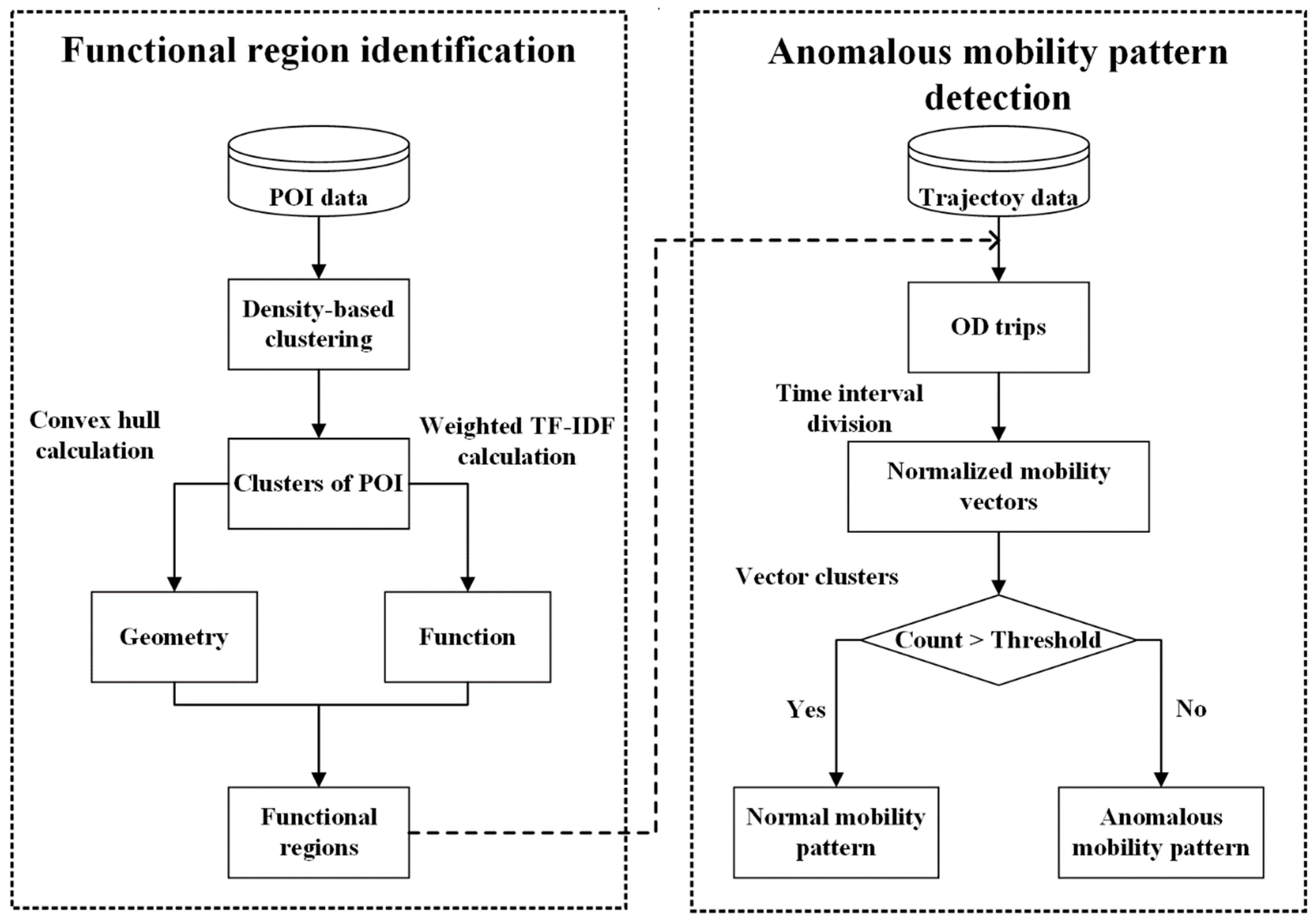
3.2. Framework of Anomalous Urban Mobility Pattern Detection

In this section, a framework is proposed to detect anomalous urban mobility patterns based on GPS trajectories and POI data. The flowchart of the framework is illustrated in Figure 1. In this figure, the framework is composed of two main steps. The first step is functional region identification. DBSCAN, a density-based clustering algorithm, is used to aggregate POIs into clusters, where each cluster is considered as a functional region. The boundary of a functional region is identified by the convex hull of the corresponding cluster. The function values of each functional region are calculated by the proposed weighted TF-IDF technique. The second step is anomalous urban mobility pattern detection. OD trips are extracted from GPS trajectories by identifying the origin and destination functional regions. Next, mobility vectors are established and normalized in each time interval. To detect anomalous urban mobility patterns, the mean shift clustering algorithm is used to aggregate the mobility vectors into different mobility patterns. Last, a threshold is calculated based on the frequencies of mobility vectors in the detected mobility patterns. A mobility pattern is considered an anomalous urban mobility pattern if the frequency of mobility vectors is smaller than the threshold.

3.3. Functional Region Identification

In this section, the DBSCAN algorithm and the weighted TF-IDF are used to identify functional regions based on POI data.

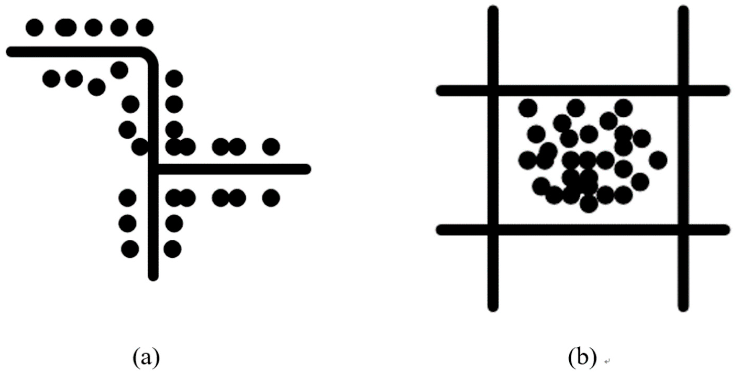
3.3.1. DBSCAN Algorithm for POI Clustering

POIs are significant components in functional regions. In this paper, functional regions based on POIs are generated. First, it is assumed that regions where POIs are densely located are usually the centers or sub-centers in a city. The centers/sub-centers with denser POIs may generate more human movement activities in the urban area. Thus, POI clusters are expected to have large density. POIs may also be distributed in different spatial forms, as shown by the example in Figure 2. In Figure 2a, POIs are distributed along the street, while POIs in Figure 2b are concentrated around one center. A density-based clustering method can detect clusters with an arbitrary shape and maintain the spatial form of POIs. Hence, DBSCAN is adopted to discover clusters of POIs.

DBSCAN identifies clusters for spatial data based on density and requires two parameters: ε, which describes the maximum distance of a neighborhood, and MinPts, which describes the Minimum number of Points required to form a dense neighborhood. In this paper, the sorted $k$-distance graph [23] is used to set the parameters of DBSCAN. In the sorted $k$-distance graph, $k$ is the parameter of MinPts. Given the value of $k$, the minimum distance for each spatial point to become a core point is calculated and called $k$-distance. In the graph, the x-axis is POIs in descending order of $k$-distance; the y-axis is the corresponding $k$-distance. The valley of the sorted $k$-distance graph might indicate proper parameters for clustering. An obvious valley, however, may not always exist for some datasets. Hence, a threshold is set in this paper. Given a ratio $r_0$, the parameter $\epsilon$ can be determined by the following equation,

$$\epsilon =\underset{d}{\mathrm{Argmin}}r\left(d\right)\ge r_0$$

(1)

where $d$ is the $k$-distance and $r\left(d\right)$ is the ratio of the number of POIs where the $k$-distance is smaller than $d$ as compared to the total number of POIs. After clustering, the convex hull for each cluster of POIs is calculated to represent the corresponding region.

3.3.2. Weighted TF-IDF for Function Value Calculation

TF-IDF is a numerical statistic that can reflect the significance of a word for a document given a corpus. It is often used as a weighting factor in information retrieval, text mining and user modeling [24]. In an urban mobility study, TF-IDF is also adopted to calculate function values in functional regions [12]. Specifically, TF corresponds to the significance of a function in the functional region, which is simply proportional to the frequency of the POIs with this function. IDF reflects the significance of the function in the whole urban area by considering the frequency of functional regions containing the function.

The conventional TF-IDF, however, cannot make an effective estimate of the function values of regions, as the impact of feature POIs on function values is not considered. For instance, railway stations belong to the function of transportation; they are rare yet important in a city. Based on the conventional TF-IDF [24], the TF-IDF value of transportation is small in the regions where railway stations are located, which is unreasonable as the conventional method treats railway stations as normal POIs with a transportation function. Therefore, the conventional TF-IDF value cannot reflect the significance of feature POIs for function estimation over the whole urban area.

To estimate a region’s function values more effectively, an extension of the TF-IDF value, called the Weighted TF-IDF (WTF-IDF), is used to calculate the functions a region provides by considering feature POIs. WTF-IDF is a product of three statistics: term frequency, inverse document frequency and an initial weight. The initial weight considers the significance of feature POIs in the whole urban area, such as railway stations.

The function calculation consists of two steps. The first step is to calculate the WTF-IDF value based on POI categories. The feature POIs and their categories are assigned a larger initial weight for function value calculation. The second step is to calculate the function value based on the categories belonging to this function. Formally, the concepts can be defined in the context of POI-based functional regions.

Definition 4.

Term frequency: The term frequency of a category $ctg{y}_i$ in the functional region $reg$ is denoted as $\mathrm{tf}\left(ctg{y}_i,reg\right)$, which corresponds to a weight of $ctg{y}_i$ provided by the POIs in the region and is proportional to the frequency of the POIs with the category $ctg{y}_i$. It is calculated in Equation (2),

$$\mathrm{tf}\left(ctg{y}_i, reg\right)=\frac{frq\left(ctg{y}_i,reg\right)}{n}$$

(2)

where $frq\left(ctg{y}_i,reg\right)$ is the frequency of POIs with the category $ctg{y}_i$ in the region $reg$ and $n$ is the total number of POIs in $reg$.

Definition 5.

Inverse document frequency: The inverse document frequency of a category $ctg{y}_i$ in the functional region $reg$ is denoted as $\mathrm{idf}\left(ctg{y}_i, reg\right)$, which is another significant indicator of $ctg{y}_i$ in the region $reg$. Inverse document frequency considers the significance of a category in the whole urban area by considering the frequency of the regions containing the category. To be more specific, a category should have a larger value in the functional region if very few regions provide this category in the whole urban area. It is calculated in Equation (3),

$$\mathrm{idf}\left(ctg{y}_i, reg\right)=\log \frac{\left|REG\right|}{N}$$

(3)

where $\left|REG\right|$ is the cardinality of the set $REG$; namely, the total number of functional regions in $REG$. $N$ stands for the number of regions providing the category $ctg{y}_i$. If fewer functional regions provide the category $ctg{y}_i$ in the whole urban area, this means a larger significance of $ctg{y}_i$ in functional regions.

As mentioned above, given a dataset of POIs, some feature POIs are important, but their frequencies are very small, such as railway stations, administrative offices and tourism sites. Therefore, the importance of these POI categories should be strengthened with an initial weight.

Definition 6.

Initial weight: Given a functional region with a set of POIs, an initial weight for a category is defined as,

$$\mathrm{weight}\left(ctg{y}_i\right)=\log \frac{\left|POI\right|}{\left|ctg{y}_i\right|}$$

(4)

where $\left|POI\right|$ is the total number of POIs in the entire urban area and $\left|ctg{y}_i\right|$ means the total number of POIs with the category $ctg{y}_i$. The initial weight can effectively reflect the significance of feature POIs, as their number is usually very small in the whole urban area.

The WTF-IDF value of a category $ctg{y}_i$ in a region $reg$ is calculated as the product of the TF value of $ctg{y}_i$ in $reg$, the IDF value of $ctg{y}_i$ in $reg$ and the initial weight of $ctg{y}_i$.

Definition 7.

Weighted Term Frequency-Inverse Document Frequency (WTF-IDF): The WTF-IDF of a category $ctg{y}_i$ in a region $reg$ is the product of TF-IDF of the category in the region and the initial weight of the category. It measures the significance of a POI category in a region and is denoted as:

$$\mathrm{WTF}–\mathrm{IDF}\left(ctg{y}_i,reg\right)=\mathrm{tf}\left(ctg{y}_i,reg\right)\times \mathrm{idf}\left(ctg{y}_i,reg\right)\times \mathrm{weight}\left(ctg{y}_i\right)$$

(5)

With the WTF-IDF value of each category, the WTF-IDF value of each function can be calculated by a summation of WTF-IDF values of categories belonging to this function.

$$\mathrm{WTF}–\mathrm{IDF}\left(fun{c}_i,reg\right)={\displaystyle \sum }_{ctg{y}_j\in fun{c}_i}\mathrm{WTF}–\mathrm{IDF}\left(ctg{y}_j,reg\right)$$

(6)

After WTF-IDF values of each function in functional regions are calculated, each region $reg$ is associated with a function vector $f_{reg}$. WTF-IDF values in the function vector are normalized between zero and one; each value indicates the significance of the corresponding function in this region.

3.4. Anomalous Mobility Pattern Detection

In this section, an effective method is proposed to detect anomalous urban mobility patterns at different temporal scales, such as by day or hour, based on GPS trajectories. As the destination of OD is an important indicator for urban mobility flows, in this paper, the anomalous urban mobility pattern detection is studied based on destinations of ODs.

The time span $T$ of a trajectory dataset can be divided into different time intervals at a specific temporal scale, denoted as $T=\left\{t_i\right\}$, where $i=0,1,2,\dots ,n$, and $t_i$ means the ith time interval. For instance, one week of data can be divided into seven time intervals by day or 168 time intervals by hour.

First, each GPS trajectory is taken as a trip and represented as an OD by identifying its origin functional region, destination functional region, start time interval and end time interval. Therefore, a set of ODs can be extracted from a GPS trajectory dataset. Next, mobility vectors are built from the extracted ODs.

Definition 8.

Mobility vector: Given $m$ functional regions in the urban area, a column vector with size $m\times 1$, called the mobility vector, is established for each time interval $t_i$. The mobility vector is denoted as $v_i$ in Equation (7),

$$v_i=\left(\begin{array}{c}\begin{array}{c}frq\left(re{g}_1,t_i\right)\\ frq\left(re{g}_2,t_i\right)\end{array}\\ ⋮\\ frq\left(re{g}_m,t_i\right)\end{array}\right)$$

(7)

where $t_i$ is the time interval associated with the mobility vector and $frq\left(re{g}_j,t_i\right)$ stands for the total frequency of ODs, which starts from the time interval $t_i$. Their destination is the region $re{g}_j$. Namely, $frq\left(re{g}_j,t_i\right)=\sum od.frq$ where $od.t_o=t_i$ and $od.re{g}_d=re{g}_j$. The mobility vector represents the spatial distribution of urban mobility flows at a time interval.

As the total frequency of OD trips has a large difference in time intervals, each mobility vector is normalized as in Equation (8),

$$v_i=\left(\begin{array}{c}\begin{array}{c}w\left(re{g}_1,t_i\right)\\ w\left(re{g}_2,t_i\right)\end{array}\\ ⋮\\ w\left(re{g}_m,t_i\right)\end{array}\right),w\left(re{g}_j,t_i\right)=\frac{frq\left(re{g}_j,t_i\right)}{{\sum }_{k=1}^{m}frq\left(re{g}_k,t_i\right)}$$

(8)

Next, the mean shift algorithm [25] is applied to generate clusters based on the established mobility vectors. Many clustering algorithms require certain prior knowledge of the dataset, such as K-means, but the prior knowledge of mobility vectors is unavailable in most occasions. The mean shift algorithm is a non-parametric clustering method and does not require any prior knowledge. The mean shift algorithm, an iterative procedure, can find the local maxima based on the density of a set of data. Kernel Density Estimation (KDE) is used for density estimation of the given dataset. As the number of discovered functional regions might be large, however, the established mobility vector would have a high dimension, which may affect the performance of the mean shift algorithm due to the curse of dimensionality. Hence, Principal Component Analysis (PCA) is applied to reduce the dimension of mobility vectors before the mean shift clustering is applied.

Given the set of $n$ mobility vectors $\left\{v_1,v_2,\dots ,v_n\right\}$ within an m-dimensional space $R^m$, the mean shift procedure iteratively updates the vector $v$ with the sample mean $M\left(v\right)$, which can be represented as:

$$M\left(v\right)=\frac{{\sum }_{i=1}^{n}K\left(v_i-v\right)v_i}{{\sum }_{i=1}^{n}K\left(v_i-v\right)}$$

(9)

where $K(·)$ is the kernel function. In this paper, the flat kernel, a frequently-used kernel for mean shift algorithm, is adopted and denoted in Equation (10).

$$K\left(v\right)=\{\begin{array}{c}1, if \Vert v\Vert \le \lambda \\ 0, if \Vert v\Vert >\lambda \end{array}$$

(10)

where $\lambda$ is the bandwidth. To estimate the value of the bandwidth, the distance between each pair of $n$ vectors is first calculated. Next, bandwidth is set as the product of the mean distance and a quantile, which normally is set to 0.3 [26].

The pseudocode of the algorithm for mobility vector clustering is displayed in Algorithm 1. The mean shift algorithm iteratively shifts a mobility vector in the direction of the maximum increase of density until it reaches the peak of its nearest KDE surface peak (cluster center). Lines 3–15 perform the mean shift procedure for each mobility vector in the dataset. Line 16 extracts the cluster centers after the mean shift procedure. Lines 17–19 label each mobility vector with the corresponding cluster center.

Algorithm 1: Mean shift clustering algorithm for mobility vectors.
Input: the set of mobility vectors $V$, the bandwidth $\lambda$, the stop threshold $stop\_thresh$
Output: the clustering result of $V$
1:	$C\leftarrow \left\{\right\}$ //store the final value of each mobility vector after the mean shift procedure
2:	$i\leftarrow 0$
3:	Foreach$v$in$V$
4:	$mean\leftarrow v$
5:	While $True$ do
6:	$nbrs\leftarrow radius\_neighbors\left(mean,\lambda \right)$ //Search all vectors within the radius
7:	$old\_mean\leftarrow mean$
8:	$mean\leftarrow SampleMean\left(mean\right)$ //Calculate the mean vector of neighbors
9:	If $\left|mean-old\_mean\right|<stop\_thresh$ Then
10:	$C\left[i\right]\leftarrow mean$
11:	$i\leftarrow i+1$
12:	Break
13:	End If
14:	End While
15:	End Foreach
16:	$centers\leftarrow unique\left(C\right)$  // Extract the cluster centers from the set $C$
17:	Foreach$v$in$V$
18:	$v.cluster\_label\leftarrow find\_nearest\_center\left(centers, v\right)$
19:	End Foreach

As mentioned above, each mobility vector $v_i$ is a vector with $m$ dimensions. With the mean shift algorithm, the mobility vectors are aggregated into $k$ clusters, and the cosine similarity between mobility vectors in the same cluster is usually larger than the cosine similarity between the mobility vectors in different clusters.

Definition 9.

Mobility pattern: A mobility pattern corresponds to a cluster of mobility vectors that are derived from OD of trips. The mobility pattern can be represented as the center vector of the cluster. Since the occurrence of anomalous mobilities are usually far less than normal mobilities, we assume that the clusters with a smaller size (less frequent patterns) could be considered as anomalous urban mobility patterns. For a mobility pattern, if the number of mobility vectors is larger than a threshold, the mobility pattern is classified as a normal urban mobility pattern. Otherwise, it will be identified as an anomalous urban mobility pattern.

In this study, given $n$ mobility vectors, $k$ clusters (mobility patterns) are generated by the mean shift algorithm. For the ith cluster $c_i$, the number of mobility vectors in $c_i$ is denoted as $\left|c_i\right|$. In order to identify normal urban mobility patterns and anomalous urban mobility patterns, the mean value of the number of the mobility vectors among the clusters is calculated and denoted as ${\left|c\right|}_{mean}$. The mobility pattern with the largest number of mobility vectors is identified, and its number of mobility vectors is denoted as ${\left|c\right|}_{max}$. To identify an anomalous urban mobility pattern, as the maximum value and mean value are significant statistics, a threshold is determined based on the maximum and mean value of the number of mobility vectors among the mobility patterns and is denoted in Equation (11).

$$threshold={\left|c\right|}_{max}-{\left|c\right|}_{mean}$$

(11)

4. Case Study

This section conducts a case study to identify functional regions and to detect anomalous urban mobility patterns based on taxi GPS trajectory data and POI data in Wuhan, China.

4.1. Dataset

Wuhan is the capital of Hubei province; its longitude and latitude are from 29.969° N–31.362° N and 113.702° E–115.083° E, respectively. The study area contains 12 sub-administrative areas in total.

Based on the Baidu map API [27], 247,538 POIs were crawled from the Baidu map in September 2017. According to the taxonomy of the Baidu map, the POI dataset can be divided into 139 categories. These categories were grouped into 17 types of functions, including public services, education, entertainment, restaurant, shopping, transportation, government, cultural media, financial services, company business, beauty service, sporting, medical services, resident area, hotel, scenic spot and automobile service.

Table 1. POI samples.

ID	Name	Function Type	Category Type	Location
1	Fu Meng market	Shopping	Super market	113.712° E, 30.405° N
2	Wuhan University	Education	University	114.359° E, 30.540° N
3	ICBC	Financial services	Bank	113.775° E, 30.238° N
4	Cheng Gong hospital	Medical services	Hospital	113.717° E, 30.406° N
5	ICBC ATM	Financial services	ATM	113.849° E, 30.264° N

shows the POIs samples.

The taxi GPS trajectory dataset, containing more than 477 million GPS points, was collected from September 1, 2013–October 31, 2013 in Wuhan. The format of GPS points included the taxi ID, longitude, latitude, timestamp, direction, speed and status. The sampling rate of the GPS trajectories was approximately 30 seconds. Due to GPS error, there existed some GPS points where latitude and longitude are zero or outside the city; these GPS points were removed from the dataset as noise. Then, 1,529,944 GPS trajectories were extracted from the dataset.

It can be noted that POI data and GPS trajectory data were not collected in the same time. In this paper, we assume that the majority of POIs in a city do not change significantly over a few years. Thus, the POI data and GPS trajectory data were integrated to study anomalous urban mobility pattern detection.

4.2. Functional Region Identification

This section investigates the effectiveness of functional region identification with the proposed method based on POIs.

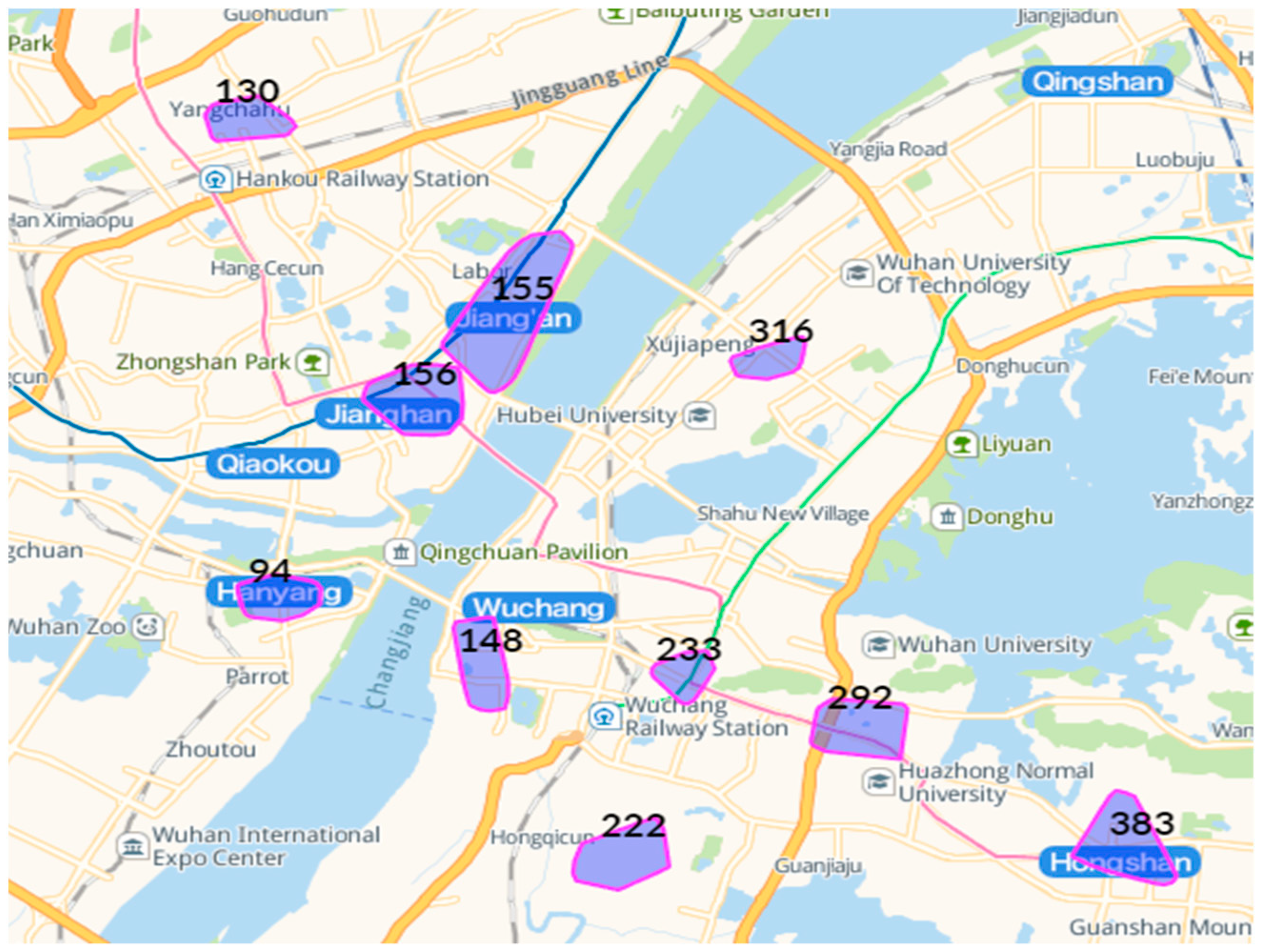
4.2.1. Functional Region Identification Based on DBSCAN and WTF-IDF

DBSCAN was used to generate clusters of POIs. The ratio threshold $r_0$ was set as 0.3; the parameters $\epsilon$ and MinPts were varied, to group POIs into clusters. The statistics of the number of POIs in functional regions appear in

Table 2. The number of generated functional regions and their POIs with varied $\epsilon$ and MinPts.

.ε, MinPts	Number of Functional Regions	Number of POIs in Functional Region
		Min.	Avg.	Max.
42, 16	2118	16	56	1543
68, 32	880	32	136	3629
109, 64	434	64	281	5169
224, 128	141	128	1201	33,184

. It can be observed in the table that given $r_0=0.3$, the value of ε grew from 42 to 224 when MinPts rose from 16 to 128. The number of generated functional regions decreased with the increase of MinPts.

To study anomalous urban mobility patterns, the parameters $\epsilon$ and MinPts were set as 64 and 109, respectively, as the sizes of generated functional regions were moderate. In Table 2, 434 functional regions were generated when $\epsilon$ = 64 and MinPts = 109. The top 10 functional regions with the largest number of POIs are shown in Figure 3. The number marked on each region represents the ID of the functional region.

A pie chart shows the function values of the functional regions. Figure 4 gives two examples. Figure 4a demonstrates the function value distribution of Region 155. The top three functions in this region are entertainment, public service and scenic spot, and the WTF-IDF values were 0.228, 0.146 and 0.108, respectively. Figure 4b demonstrates the function value distribution of Region 156. Its top three functions are public service, entertainment and beauty service, and the WTF-IDF values were 0.156, 0.122 and 0.112, respectively. It could be observed that the two functional regions had different function value distributions, although both of them are located in a prosperous urban area and are close to each other.

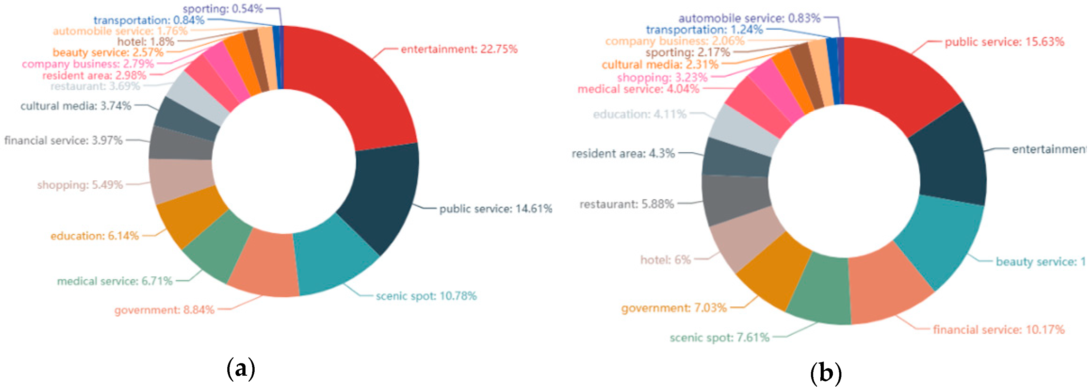
4.2.2. Performance Comparison between WTF-IDF and TF-IDF

In this section, the effectiveness of the proposed WTF-IDF and the conventional TF-IDF is investigated. After identifying the functional regions with DBSCAN, both conventional TF-IDF and the proposed WTF-IDF were calculated for every region. The five regions with the smallest cosine similarity between TF-IDF and WTF-IDF were selected, and we invited local people to label the top two leading functions of each region in a similar way as in [11]. The regions’ functions are shown in

Table 3. The five regions with the smallest cosine similarity between TF-IDF and Weighted TF-IDF (WTF-IDF) and their top three functions.

Region ID	Top Three Leading Functions				Function Label
	TF-IDF		WTF-IDF
56	Entertainment	0.23	Transportation	0.38	Transportation Automobile service
	Transportation	0.21	Automobile service	0.18
	Shopping	0.20	Entertainment	0.17
279	Government	0.19	Cultural media	0.26	Cultural media Government
	Cultural media	0.15	Public services	0.17
	Public services	0.15	Government	0.15
5	Shopping	0.38	Entertainment	0.28	Entertainment Shopping
	Restaurant	0.21	Shopping	0.27
	Entertainment	0.20	Tourism	0.19
192	Public services	0.21	Medical services	0.27	Medical services Resident area
	Medical services	0.17	Public services	0.24
	Entertainment	0.16	Entertainment	0.17
227	Resident area	0.28	Public services	0.23	Resident area Entertainment
	Entertainment	0.19	Resident area	0.22
	Public services	0.16	Entertainment	0.21

, and their basic information is given in

Table 4. The basic information of the five regions.

Region ID	Number of POIs	Center
		Latitude	Longitude
56	114	30.773° E	114.205° N
279	65	30.365° E	114.329° N
5	71	30.567° E	114.053° N
192	65	30.604° E	114.287° N
227	67	30.503° E	114.323° N

.

It can be observed in Table 3 that WTF-IDF had better performance than TF-IDF for function estimation in most regions. After scrutinizing the POIs in each region, it was discovered that WTF-IDF can capture the significance of feature POIs. For instance, the feature POI was Tianhe International Airport in Region 56, Jiangxia Television Media in Region 279 and Wuhan No.6 Hospital in Region 192. However, the conventional TF-IDF took these feature POIs as normal POIs and underestimated their significance for the region’s function.

4.3. Anomalous Urban Mobility Pattern Detection

This section studies anomalous urban mobility patterns based on the discovered functional regions and OD trips in Wuhan. An overview of the spatio-temporal distribution of OD trips was first studied; anomalous urban mobility patterns were detected and discussed at different temporal scales.

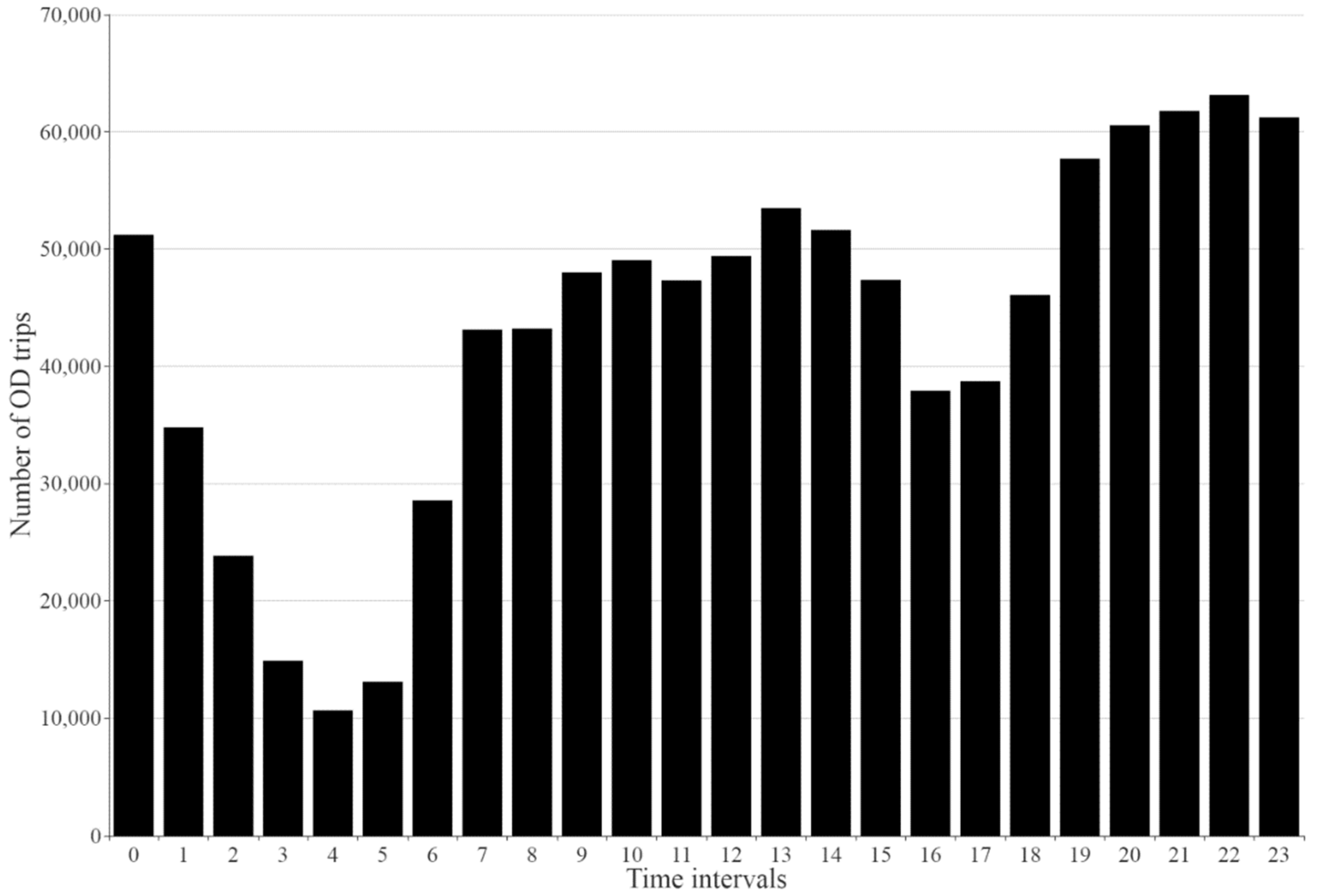
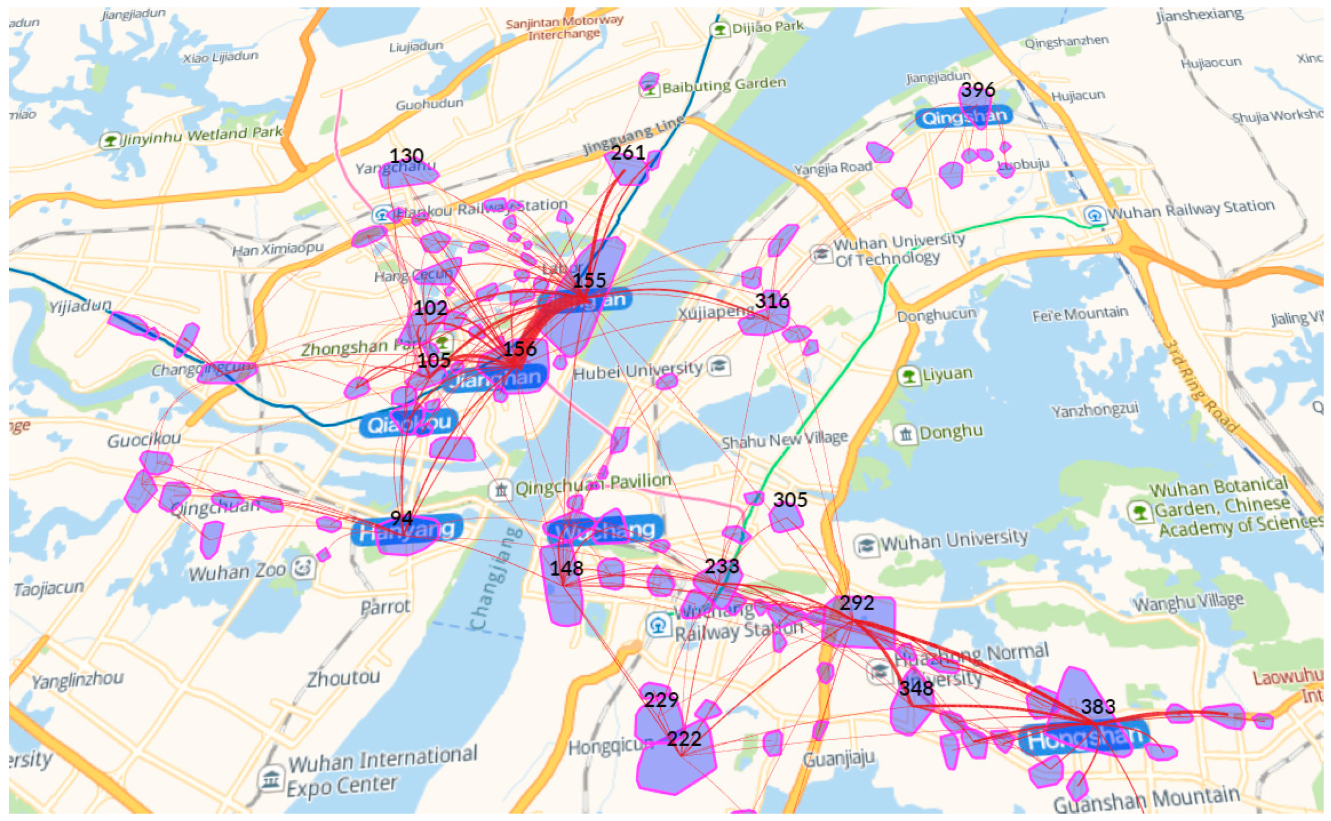
4.3.1. Distribution of OD Trips

The distribution of the number of OD trips per hour is shown in Figure 5. The x-axis presents one-hour time intervals ranging from 0–23. For example, 0 stands for 0:00–1:00 and 1 stands for 1:00–2:00. The y-axis represents the number of OD trips occurring during the time interval.

As shown in Figure 5, the lowest level of mobility in Wuhan was between 3:00 and 5:00, and the peaks of movement were at 7:00–14:00 and 19:00–23:00, which reflects the temporal pattern of overall urban mobility in the city.

The frequency of the functional regions as the origin and destination of OD trips was studied to identify hotspot regions. The top 10 origin and destination regions are listed in

Table 5. Top 10 hot functional regions.

Origin			Destination
Region ID	Frequency	Leading Function	Region ID	Frequency	Leading Function
155	90,023	Entertainment	155	86,778	Entertainment
156	48,965	Public service	156	57,343	Public service
383	32,052	Entertainment	292	32,537	Education
292	30,286	Education	383	32,287	Entertainment
105	26,932	Entertainment	105	25,213	Entertainment
94	19,875	Public service	233	21,720	Public service
233	19,161	Public service	148	20,793	Public service
148	18,689	Public service	102	18,267	Entertainment
102	18,208	Entertainment	94	17,853	Public service
316	16,151	Entertainment	348	15,916	Entertainment

.

As observed in Table 5, the top 10 functional regions as the origin or destination of OD trips were similar, with the leading functions being entertainment or public service. Regions 155 and 156, as the origin and destination of OD trips, had the highest level of mobility.

Urban mobility is seen on the map in Figure 6. The polygons represent the geometry of the functional regions. The OD trips are represented by the red line. The wider line indicates the larger frequency of OD trips between the two functional regions. Figure 6 reveals that Regions 155 and 156 had the largest number of OD trips, which corresponds with Table 5.

In the next sections, anomalous urban mobility patterns are studied at different temporal scales. As the dataset contained the trajectory data of 61 days, anomalous urban mobility patterns were studied at the scale of day and hour. Based on local news, certain urban mobility patterns during China’s National Day and Mid-Autumn Festival holiday differ from normal days’ patterns. Therefore, these dates were taken as the ground truth to validate if the proposed method can detect the dates effectively.

4.3.2. Anomalous Urban Mobility Pattern at the Scale of Day

At the scale of day, a mobility vector was constructed for each day. The mobility vector dimension was 434, corresponding to the number of identified functional regions. After dimension reduction with PCA and clustering with the mean shift clustering, four clusters were discovered, denoted as $D_1$, $D_2$, $D_3$, and $D_4$. The number of mobility vectors in the four clusters was 52, 5, 1 and 3, respectively. The mean value of the number of mobility vectors among the clusters was 15.25. Thus, the threshold to discriminate an anomalous urban mobility pattern was set as 36.75. Only $D_1$ was considered as a normal urban mobility pattern, while the other clusters were considered as anomalous urban mobility patterns.

Close examination of the anomalous urban mobility patterns revealed that $D_2$ had five dates including September 20, October 2, October 3, October 4 and October 5. Of these, September 20 was the last date of the Mid-Autumn Festival holiday; the other four days were during China’s National Day holiday, from October 1– October 7. $D_3$ contained only one day, October 1, which is the holiday’s start date. $D_4$ contained the first two days of the Mid-Autumn Festival holiday (September 18, September 19) and the day before China’s National Day (September 30). Therefore, it can be inferred that the anomalous urban mobility patterns in this dataset all occurred around holidays when people may visit their family and friends or go out of the city for a vacation.

To understand the clustering results of these mobility vectors intuitively, a $61\times 61$ similarity matrix was constructed, based on the cosine similarity between mobility vectors, visualized by the heatmap in Figure 7. Two obvious bands appeared around September 19 and September 30, which means that the similarity of mobility between these dates and the mobility on the other dates was small. The mobility on October 1 had the smallest similarity with the mobility on other dates, as shown by the blue band in the figure.

As mentioned above, each cluster center was taken as the representative of a corresponding mobility pattern. To discover the difference of the spatial distribution between the normal urban mobility pattern and the anomalous urban mobility patterns, the difference vectors, denoted as $V_2$, $V_3$ and $V_4$, were calculated between the cluster center of $D_1$ and the cluster centers of $D_2$, $D_3$ and $D_4$. Each element in the vector represents the difference of functional regions as destinations of OD trips. Figure 8a–c shows the top 10 functional regions, with the largest difference value in $V_2$, $V_3$ and $V_4$, respectively.

In Figure 8, the x-axis stands for the functional region ID, and the y-axis represents the values in $V_2$, $V_3$ and $V_4$. The regions with the largest positive value in $V_2$, $V_3$ and $V_4$ were Regions 105, 119 and 119, which means that a large mobility increase in $D_2$, $D_3$ and $D_4$ existed in the corresponding Regions 105, 119 and 119 compared with $D_1$, respectively. The leading functions of Region 105 are entertainment and public service. According to the map, Region 105 is a prosperous area, comprising a large park (Zhongshan Park) and five shopping malls. Similarly, the leading functions of Region 119 are hotel and transportation; Hankou railway station, a major railway station in Wuhan, is located in Region 119. Compared with the normal mobility pattern, the anomalous urban mobility patterns mainly flowed to the entertainment area and transportation center.

4.3.3. Anomalous Urban Mobility Pattern at the Scale of Hour

This section studies the anomalous urban mobility pattern at the scale of hour. First, the OD trips were divided into $61\times 24=1464$ time intervals. Similar to the scale of day, a mobility vector was established for each hour, so 1464 mobility vectors were obtained. After mean shift clustering, seven clusters were generated and denoted as $H_1$, $H_2$, …, $H_7$. The number of mobility vectors in these clusters was 1377, 40, 11, 3, 1, 20 and 11, respectively. As the largest value and the mean value were 1377 and 209.1, the threshold to differentiate anomalous urban mobility patterns was set as 1167.9. Therefore, cluster $H_1$ was considered as the normal urban mobility pattern, whereas the other clusters were considered as anomalous urban mobility patterns.

Compared with the experimental results at the scale of day, more anomalous urban mobility patterns were detected at the scale of hour. The detected anomalous mobility patterns were different at the two temporal scales. One example is the mobility pattern on October 1. At the scale of day, October 1 belonged to the anomalous mobility pattern $D_3$. At the scale of hour, however, three time intervals (5:00–6:00, 6:00–7:00 and 7:00–8:00) for October 1 belonged to the anomalous mobility pattern $H_2$. All other time intervals for October 1 belonged to the normal urban mobility pattern $H_1$. The difference illustrates that the anomalous mobility pattern mainly occurred between 5:00 and 8:00 on October 1. Another example is September 19. At the scale of day, September 19 was clustered into the anomalous mobility pattern $D_4$. At the scale of hour, three time intervals (5:00–6:00, 6:00–7:00 and 7:00–8:00) for September 19 belonged to the anomalous mobility pattern $H_2$, one time interval (4:00–5:00 am) belonged to the anomalous mobility pattern $H_5$, and all other time intervals belonged to the normal mobility pattern $H_1$. Thus, studying anomalous urban mobility patterns with a reasonable temporal scale was significant for different scenarios.

4.3.4. Anomalous Urban Mobility Pattern Based on a Grid

This section studies the performance of the proposed anomalous urban mobility pattern detection method based on a grid. The study area was partitioned into 19,866 functional regions based on a 1 km × 1 km grid. Out of them, there were 4066 functional regions that were the destination of OD trips. Thus, the mobility vector dimension was 4066. With the mean shift algorithm, mobility vectors were grouped into seven clusters, denoted as $G{D}_1$, $G{D}_2$, $G{D}_3$, $G{D}_4$, $G{D}_5$, $G{D}_6$ and $G{D}_7$. Based on the threshold, six clusters were taken as anomalous mobility patterns and are shown in

Table 6. Anomalous urban mobility patterns’ detection based on a grid.

Anomalous Urban Mobility Patterns Based on Grid		Anomalous Urban Mobility Patterns Based on DBSCAN Clustering
$G{D}_2$	October 2–October 6	$D_2$	September 20, October 2–October 5
$G{D}_3$	October 1	$D_3$	October 1
$G{D}_4$	September 18, September 30	$D_4$	September 18, September 19, September 30
$G{D}_5$	October 7, October 8
$G{D}_6$	September 19
$G{D}_7$	September 20

.

In Table 6, more anomalous urban mobility patterns were detected based on the grid, compared with the patterns detected based on DBSCAN clustering. For instance, $D_4$ generated from DBSCAN clustering, was further divided into two patterns $G{D}_4$ and $G{D}_6$ based on the grid; $D_2$ from DBSCAN clustering was further divided into two patterns $G{D}_2$ and $G{D}_7$ based on the grid. Besides, the grid-based method discovered two dates, October 6 and October 7, that were not detected based on DBSCAN clustering. Thus, the proposed anomalous urban mobility pattern method performed even better based on the grid than DBSCAN clustering. The reason is that, compared with the grid, the functional regions generated by DBSCAN cannot cover the entire study area so that a large amount of information of trips was lost.

Next, the semantic meaning of the discovered anomalous mobility pattern based on the grid was studied. For each anomalous pattern, the top three regions with the largest mobility increase is shown in

Table 7. Top three regions with the largest mobility increase for each anomalous pattern based on the grid.

Anomalous Pattern	Region IDs
$G{D}_2$	10774	11796	11925
$G{D}_3$	10774	11796	11925
$G{D}_4$	10774	11796	11925
$G{D}_5$	10774	10629	8432
$G{D}_6$	11796	11925	10629
$G{D}_7$	11796	11147	10629

.

Based on WTF-IDF, the leading functions of Regions 10774, 11796, 11925, 10629, 8432, and 11147 were restaurant, public services, public services, hotel, shopping and beauty, respectively. However, the large mobilities in the regions were not caused by these leading functions after close examination of POIs in the regions. For Regions 10744, 11796, 11925, 10629 and 8432, the leading function should be transportation, which causes the large mobility, because the feature POI is Wuhan Railway station in Region 10744, Fujiapo Bus station center in Region 11796, Wuchang Railway station in Region 11925, Hankou Railway station in Region 10629 and Tianhe International Airport in Region 8432.

Therefore, the functional regions generated by the grid cannot reflect its leading function effectively based on WTF-IDF, which makes it difficult to understand the semantic meaning of anomalous mobility patterns. The reason is that the spatial structure of functional regions is not considered by the grid-based method. One functional region might be divided into two functional regions or multiple functional regions merged into one functional region based on the grid, which leads to the ineffective estimation of region’s function.

5. Conclusions and Future Works

Anomalous urban mobility pattern detection is an important topic in studies of urban mobility. In this paper, a framework was proposed to detect anomalous urban mobility patterns based on GPS trajectories and POI data. The DBSCAN algorithm and weighted TF-IDF technique were used to identify functional regions; anomalous urban mobility patterns were differentiated from normal urban mobility patterns after mobility vector clustering. Furthermore, anomalous urban mobility patterns can be detected at different temporal scales. To validate the proposed framework, experiments were conducted on a real dataset in the city of Wuhan, China.

Some improvements can be made based on this study. First, current functional region identification depends only on the distribution of POIs. The identified functional regions are areas with dense POIs, while the areas with sparse POIs are ignored. Mobility between the regions with sparse POIs will be considered in anomalous urban mobility pattern detection. Second, anomalous urban mobility patterns may vary with different spatial scales. In the future, we will study urban mobility patterns and detect anomalous urban mobility patterns at different spatial scales. Third, we will compare the performance of the proposed anomalous urban mobility detection method with related research works in this area.

References

1. Liu, Y.; Wang, F.; Xiao, Y.; Gao, S. Urban land uses and traffic “source-sink areas”: Evidence from GPS-enabled taxi data in Shanghai. Landsc. Urban Plan. 2012, 106, 73–87. [Google Scholar] [CrossRef]
2. D’Andrea, E.; Marcelloni, F. Detection of traffic congestion and incidents from GPS trace analysis. Expert Syst. Appl. 2017, 73, 43–56. [Google Scholar] [CrossRef]
3. Wang, Y.; Gu, Y.; Dou, M.; Qiao, M. Using Spatial Semantics and Interactions to Identify Urban Functional Regions. ISPRS Int. J. Geo-Inf. 2018, 7, 130. [Google Scholar] [CrossRef]
4. Liu, X.; Ban, Y. Uncovering Spatio-Temporal Cluster Patterns Using Massive Floating Car Data. ISPRS Int. J. Geo-Inf. 2013, 2, 371–384. [Google Scholar] [CrossRef] [Green Version]
5. Yang, Y.; Heppenstall, A.; Turner, A.; Comber, A. Who, Where, Why and When? Using Smart Card and Social Media Data to Understand Urban Mobility. ISPRS Int. J. Geo-Inf. 2019, 8, 271. [Google Scholar] [CrossRef]
6. Wang, H.; Huang, H.; Ni, X. Revealing Spatial-Temporal Characteristics and Patterns of Urban Travel: A Large-Scale Analysis and Visualization Study with Taxi GPS Data. ISPRS Int. J. Geo-Inf. 2019, 8, 257. [Google Scholar] [CrossRef]
7. Cui, G.; Luo, J.; Wang, X. Personalized travel route recommendation using collaborative filtering based on GPS trajectories. Int. J. Digit. Earth 2018, 11, 284–307. [Google Scholar] [CrossRef]
8. Qu, B.; Yang, W.; Cui, G.; Wang, X. Profitable Taxi Travel Route Recommendation Based on Big Taxi Trajectory Data. IEEE Trans. Intell. Transp. Syst. 2019. [Google Scholar] [CrossRef]
9. Yue, Y.; Zhuang, Y.; Yeh, A.G.O.; Xie, J.Y.; Ma, C.L.; Li, Q.Q. Measurements of POI-based mixed use and their relationships with neighbourhood vibrancy. Int. J. Geogr. Inf. Sci. 2017, 31, 658–675. [Google Scholar] [CrossRef]
10. Wang, P.; Fu, Y.; Liu, G.; Hu, W.; Aggarwal, C. Human mobility synchronization and trip purpose detection with mixture of hawkes processes. In Proceedings of the 23rd ACM SIGKDD International Conference on Knowledge Discovery and Data Mining (KDD 2017), Halifax, NS, Canada, 13–17 August 2017; pp. 495–503. [Google Scholar]
11. Yuan, J.; Zheng, Y.; Xie, X. Discovering regions of different functions in a city using human mobility and POIs. In Proceedings of the 18th ACM SIGKDD International Conference on Knowledge Discovery and Data Mining (KDD 2012), Beijing, China, 12–16 August 2012; pp. 186–194. [Google Scholar]
12. Yuan, N.J.; Zheng, Y.; Xie, X.; Wang, Y.; Zheng, K.; Xiong, H. Discovering Urban Functional Zones Using Latent Activity Trajectories. IEEE Trans. Knowl. Data Eng. 2018, 27, 712–725. [Google Scholar] [CrossRef]
13. Qi, G.; Li, X.; Li, S.; Pan, G.; Wang, Z.; Zhang, D. Measuring social functions of city regions from large-scale taxi behaviors. In Proceedings of the IEEE International Conference on Pervasive Computing and Communications Workshops (PERCOM Workshops), Seattle, WA, USA, 21–25 March 2011; pp. 384–388. [Google Scholar]
14. Shi, L.; Gangopadhyay, A.; Janeja, V.P. STenSr: Spatio-temporal tensor streams for anomaly detection and pattern discovery. Knowl. Inf. Syst. 2015, 43, 333–353. [Google Scholar] [CrossRef]
15. Fanaee-T, H.; Gama, J. Event detection from traffic tensors: A hybrid model. Neurocomputing 2016, 203, 22–33. [Google Scholar] [CrossRef] [Green Version]
16. Lin, C.; Zhu, Q.; Guo, S.; Jin, Z.; Lin, Y.R.; Cao, N. Anomaly detection in spatiotemporal data via regularized non-negative tensor analysis. Data Min. Knowl. Discov. 2018, 32, 1056–1073. [Google Scholar] [CrossRef] [Green Version]
17. Gao, S.; Janowicz, K.; Couclelis, H. Extracting urban functional regions from points of interest and human activities on location-based social networks. Trans. GIS 2017, 21, 446–467. [Google Scholar] [CrossRef]
18. Cao, J.; Tu, W.; Li, Q.; Zhou, M.; Cao, R. Exploring the distribution and dynamics of functional regions using mobile phone data and social media data. In Proceedings of the 14th International Conference on Computers in Urban Planning and Urban Management, Boston, MA, USA, 10 July 2015. [Google Scholar]
19. Kaltenbrunner, A.; Meza, R.; Grivolla, J.; Codina, J.; Banchs, R. Urban cycles and mobility patterns: Exploring and predicting trends in a bicycle-based public transport system. Pervasive Mob. Comput. 2010, 6, 455–466. [Google Scholar] [CrossRef]
20. Peng, C.; Jin, X.; Wong, K.C.; Shi, M.; Liò, P. Collective human mobility pattern from taxi trips in urban area. PLoS ONE 2012, 7, e34487. [Google Scholar]
21. Zhang, W.; Li, S.; Pan, G. Mining the semantics of origin-destination flows using taxi traces. In Proceedings of the 2012 ACM Conference on Ubiquitous Computing-UbiComp ’12, Pittsburgh, PA, USA, 5–8 September 2012; p. 943. [Google Scholar]
22. Kuang, W.; An, S.; Jiang, H. Detecting traffic anomalies in urban areas using taxi GPS data. Math. Probl. Eng. 2015. [Google Scholar] [CrossRef]
23. Ester, M.; Kriegel, H.P.; Sander, J.; Xu, X. A Density-Based Algorithm for Discovering Clusters in Large Spatial Databases with Noise. Kdd 1996, 96, 226–231. [Google Scholar]
24. Salton, G.; Buckley, C. Term-weighting approaches in automatic text retrieval. Inf. Process. Manag. 1988, 24, 513–523. [Google Scholar] [CrossRef] [Green Version]
25. Comaniciu, D.; Meer, P. Mean shift: A robust approach toward feature space analysis. IEEE Trans. Pattern Anal. Mach. Intell. 2002, 5, 603–619. [Google Scholar] [CrossRef]
26. Pedregosa, F.; Varoquaux, G.; Gramfort, A.; Michel, V.; Thirion, B.; Grisel, O.; Blondel, M.; Prettenhofer, P.; Weiss, R.; Dubourg, V.; et al. Scikit-Learn: Machine Learning in Python. JMLR 2011, 12, 2825–2830. [Google Scholar]
27. Baidu Map API. Available online: http://lbsyun.baidu.com/index.php?title=jspopular (accessed on 20 September 2017).
Figure 1. Framework of anomalous mobility pattern detection.
Ijgi 08 00308 g001
Figure 2. The spatial distribution of POIs. (a) Along the street; (b) concentrated around a center.
Ijgi 08 00308 g002
Figure 3. Top 10 intensive functional regions.
Ijgi 08 00308 g003
Figure 4. Examples of the function distribution in functional regions. (a) Region 155; (b) Region 156.
Ijgi 08 00308 g004
Figure 5. Temporal distribution of Origin-Destination (OD) trips.
Ijgi 08 00308 g005
Figure 6. The overall view of urban mobility in Wuhan.
Ijgi 08 00308 g006
Figure 7. The similarity matrix of mobility vectors at the scale of day.
Ijgi 08 00308 g007
Figure 8. The top 10 functional regions with the largest values in (a) V 2 (b) V 3 and (c) V 4 .
Ijgi 08 00308 g008