Road Congestion Detection Based on Trajectory Stay-Place Clustering

Abstract

The results of road congestion detection can be used for the rational planning of travel routes and as guidance for traffic management. The trajectory data of moving objects can record their positions at each moment and reflect their moving features. Utilizing trajectory mining technology to effectively identify road congestion locations is of great importance and has practical value in the fields of traffic and urban planning. This paper addresses the issue by proposing a novel approach to detect road congestion locations based on trajectory stay-place clustering. First, this approach estimates the speed status of each time-stamped location in each trajectory. Then, it extracts the stay places of the trajectory, each of which is denoted as a seven-tuple containing information such as starting and ending time, central coordinate, average direction difference, and so on. Third, the time-stamped locations included in stay places are partitioned into different stay-place equivalence classes according to the timestamps. Finally, stay places in each equivalence class are clustered to mine the congestion locations of multiple trajectories at a certain period of time. Visual representation and experimental results on real-life cab trajectory datasets show that the proposed approach is suitable for the detection of congestion locations at different timestamps.

1. Introduction

Traffic congestion has become a serious problem that hinders the rapid development of modern cities. If habitually congested road sections are detected in advance, vehicles can effectively avoid spending unnecessary time on the road, greatly increasing the travel efficiency. Utilizing modern technology to effectively identify road congestion locations is of great importance and has practical value in the fields of traffic and urban planning [1,2].

With the rapid development of positioning and storage technology, large amounts of trajectory data of moving objects can be produced. These trajectories contain abundant temporal and spatial information and can be used in many information services [3,4,5,6], such as location-based services, traffic monitoring, road planning, congestion prediction, user behavior analysis, and travel recommendations [7,8,9,10,11].

Moving and staying are the two basic states of locations in trajectory data. It is well known that stay point recognition is a critical method in mining information from trajectory data, and this is, therefore, the premise of frequent location discovery, interest point mining, etc. [12,13]. Stay point recognition plays a fundamental role in trajectory analysis. Stay points are a series of actual time-stamped locations extracted from the raw trajectory data. Each stay point denotes a geographic region where an individual stays for a certain duration. On the one hand, stay points generally carry a particular semantic meaning, such as the shopping malls, restaurants, and cinemas, visited by an individual [14]. On the other hand, a vehicle is also in a state of staying when it is stuck in a traffic jam. These are two different kinds of staying states. The former is a meaningful stay, while the latter is a helpless and anxious waiting, unlike waiting for a normal signal. Therefore, the extraction of meaningless staying places based on trajectory data of vehicles can be used for road congestion detection. In this paper, we propose a methodology called Congestion Location Detection approach based on Stay-places Clustering (CLDSC) that allows the detection of congestion locations from the trajectory data of moving vehicles.

In summary, this paper makes the following contributions:

(1)

Trajectory stay model construction. By learning from the idea of stay points [14], we propose a novel trajectory stay model, which is adopted in stay place extraction and later research.

(2)

Trajectory stay places extraction. A stay place extraction algorithm is proposed based on the extraction of continuous low-speed locations and the calculation of average direction differences of each candidate stay place.

(3)

Equivalence classes partition and stay places clustering. An equivalence class partition algorithm is proposed, and a stay-place clustering algorithm based on equivalence classes is proposed to detect the optimal stay places, which can help detect road congestion locations.

(4)

Experimental Study. The proposed algorithm is tested on a real-life trajectory dataset. Visual presentation and experimental results show that our algorithm can detect road congestion locations with high accuracy.

The remainder of this paper is organized as follows. In Section 2, we introduce the related work. Section 3 introduces preliminary concepts and the problem definition. Section 4 presents a novel method for the detection of road congestion locations. Experimental results and analysis are presented in Section 5. Section 6 concludes the paper and provides future research directions.

2. Related Work

A large amount of research has been conducted on traffic congestion detection, which provides many useful insights in practical applications [10,15,16,17]. Detection methods are mainly realized based on the traffic flow of vehicles, road networks, or POIs (Points of Interests). Wang et al. [16] proposed a three-phase framework for exploring the traffic congestion correlation between road segments from multiple data sources including road networks, GPS trajectories of taxis, and POIs. This method focuses on traffic congestion correlation, and it is realized based on the congestion information on each road segment in each specific time slot. Anbaroglu et al. [15] presented a detection method for non-recurrent traffic congestion based on spatio-temporal clustering. Kong et al. [10] proposed a novel approach to estimate and predict urban traffic congestion using floating car trajectory data. This approach calculates traffic density based on traffic speed, traffic volume, and the length and lane number of the road section. Liu et al. [18] proposed a mobility-based clustering approach to detect crowded spots in city transportation. D’Andrea et al. [17] presented an expert system for the detection of traffic congestion and incidents from real-time GPS trajectories. Wang et al. [19] presented a locality-constraint distance-metric learning for traffic congestion detection to characterize the congestion level in different scenes. Therefore, a dataset that consists of 20 different scenes is constructed in their work. All the above-mentioned methods are implemented depending on both road network and vehicle information. The challenges of data collection and high computation complexity are becoming increasingly evident. The advantages and disadvantages of map matching algorithms directly affect the accuracy and reliability of the congestion detection results.

Meanwhile, many achievements have been made on the detection of stay points based on the trajectories of moving objects [14,20,21,22], which can be extended to many applications, including user behavior analysis and road planning. For example, Li et al. [23] first proposed a stay point detection algorithm based on the distance measure and time span between any two successive points. Yuan et al. [20,24] proposed an improved stay point detection algorithm based on density clustering. Zheng et al. [14] proposed a hierarchical framework to uniformly model each individual’s location history, which consists of three steps. The stay points are determined from the trajectory data in the first step. They presented a stay point detection algorithm based on two operations: checking the spatio-temporal constraint and expanding. On the one hand, the method ignores that, although the distance between two merged locations is small, the time interval may be very short; even if such locations and others form a time interval greater than the time threshold, it is not suitable for them to be merged together as a stop point. On the other hand, the selection of distance threshold is not easy due to the loss of signal in buildings. Do et al. [22] first used raw trajectory data as an input to detect stay points. Pavan et al. [25] proposed an approach to recognize important locations based on the detection of a candidate stay point and the mapping of its feature space. Stylianou et al. [26] presented a geometry-based method to extract stay points. The user’s trajectory is converted to a two-dimensional discrete time series curve, and the stay point is converted to a local minimum of the first derivative of the curve.

Cao et al. [27] extracted semantic locations from GPS data and assigned significance to the extracted locations. Kami et al. [12] proposed an algorithm that extracts significant locations based on the method of probabilistically detecting peak locations in the density distribution of data points. They also used density information to score the extracted locations according to their importance. An et al. [28] proposed a method for measuring urban recurrent congestion evolution patterns based on grid divisions and GPS-equipped vehicle mobility data. The Grid Congestion Mode (GCM) is defined based on the average velocity of all trajectories within each grid. This method is vulnerable to individual noise locations.

The above methods have achieved good results in traffic congestion detection or stay point detection. However, the intrinsic characteristics of different kinds of stay points are rarely distinguished, and the relationship between abnormal staying and congestion is not considered. During the trip, if there is a large number of abnormal waiting in a certain position at a certain time, it indicates that there is congestion at this place at this time. Therefore, road congestion detection based on stay place extraction is reasonable and feasible.

In this paper, we extract stay places and propose a new approach called CLDSC to detect road congestions. The stay place recognition method based on the extraction of continuous low-speed points extraction can effectively avoid noise interference. In addition, this method considers the average direction difference within each candidate stay place, which can better serve the detection of road congestion locations.

3. Fundamental Concept and Problem Definition

In this section, we define the concepts, notations, and corresponding calculation equations used throughout the paper.

Definition 1

(Trajectory). A trajectory is an ordered set of time-stamped locations, denoted as T:

$$T=\left\{Tid,\left(t_1,x_1,y_1\right),\left(t_2,x_2,y_2\right),\cdots ,\left(t_n,x_n,y_n\right)\right\}$$

(1)

where $t_r<t_{r+1}$ for all $1\le r<n$, $t_r$ is a timestamp, $\left(x_r,y_r\right)$ is a location in ${ℝ}^2$, $\left(t_r,x_r,y_r\right)$ is a time-stamped location which means that a moving object is at location $\left(x_r,y_r\right)$ at time $t_r$, Tid is the identifier of a trajectory representing a moving object, and n (also represented by |T|) is the number of time-stamped locations in the trajectory T.

Hereinafter, $TS=\left\{T_1,T_2,\cdots ,T_p\right\}$ is a dataset consisting of p trajectories, $T_i=\left\{i,lo{c}_1^i,lo{c}_2^i,\cdots ,lo{c}_{n_i}^i\right\}$ represents the i-th trajectory in TS, $lo{c}_w^i$ is the w-th time-stamped location of the i-th trajectory ($1\le w\le n_i, \left|T_i\right|=n_i$).

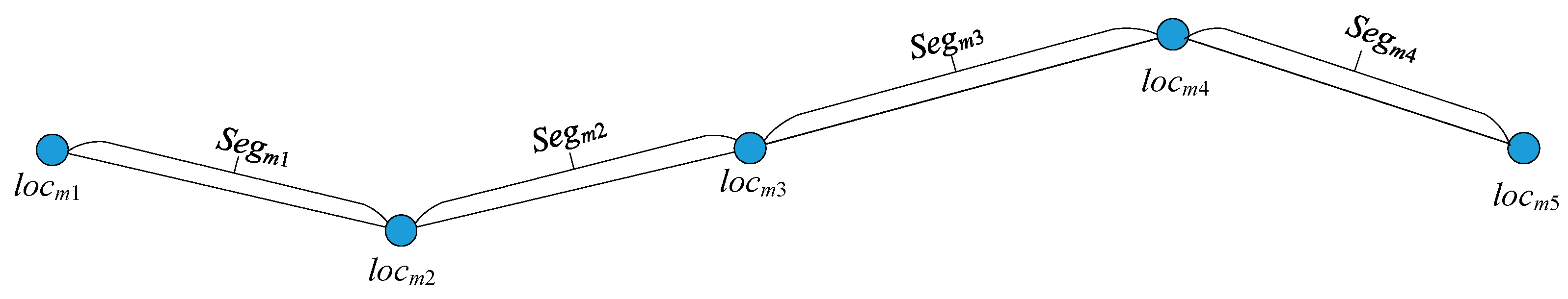
Definition 2

(Trajectory segment). Consider a trajectory T. A trajectory segment is defined as the line segment between any pair of adjacent time-stamped locations ($lo{c}_r,lo{c}_{r+1}$) in the trajectory T, $1\le r<\left|T\right|$.

Figure 1 shows an example including four trajectory segments $Se{g}_{m_i}\left(1\le i\le 4\right)$ and 5 locations $lo{c}_{m_j}\left(1\le j\le 5\right)$.

Definition 3

(Low-speed point). A low-speed point refers to a time-stamped location where a moving object is at rest, moves within a relatively small range for a long time, or moves at a very slow speed.

For example, when a user is resting, eating, visiting, shopping, waiting for traffic lights, or stuck in a traffic jam, the locations they pass are low-speed points. In this paper, low-speed points are extracted based on the speed threshold set by the experiments.

Definition 4

(Stay place). Stay place refers to a set consisting of at least three consecutive low-speed points that meet the time threshold and the average direction difference threshold requirements. The two thresholds are defined in specific applications. Consider a trajectory T, sn stay places of T can be represented as a set $SD=\left\{S_1,S_2,\cdots ,S_{sn}\right\}$, where $S_m=\left\{lo{c}_{m_1},lo{c}_{m_2},\cdots ,lo{c}_{m_{\left|S_m\right|}}\right\}$ represents the m-th stay place in T, $1\le m\le sn$.

Each stay place $S_m$ is denoted as a seven-tuple $<sn{o}_{S_m},en{o}_{S_m},s{t}_{S_m},e{t}_{S_m},x_{S_m},y_{S_m},d{d}_{S_m}>$, where $sn{o}_{S_m}$ and $en{o}_{S_m}$ respectively represent the No. of the first low-speed point and the No. of the last low-speed point in $S_m$, $s{t}_{S_m}$ and $e{t}_{S_m}$ represent the timestamp of the first low-speed point and the timestamp of the last low-speed point in $S_m$ respectively, $\langle x_{S_m},y_{S_m}\rangle$ represents the central coordinate of $S_m$, and $d{d}_{S_m}$ is the average direction difference of $S_m$. The average direction difference will be described in detail in Section 4.3.1. The calculation method for $x_{S_m}$ and $y_{S_m}$ is as follows:

$$x_{S_m}=\frac{1}{\left|S_m\right|-1}{{\displaystyle \sum }}_{i=1}^{\left|S_m\right|-1}{w}_i*seg\_x_i$$

(2)

$$y_{S_m}=\frac{1}{\left|S_m\right|-1}{{\displaystyle \sum }}_{i=1}^{\left|S_m\right|-1}{w}_i*seg\_y_i$$

(3)

where $\left|S_m\right|$ represents the number of locations in $S_m$, $\langle seg\_x_i,seg\_y_i\rangle$ represents the central coordinate of the i-th trajectory segment $Se{g}_{m_i}=\langle lo{c}_{m_i},lo{c}_{m_{i+1}}\rangle$ in $S_m$ $\left(1\le i\langle |S_m|\right)$, and $w_i$ represents the weight of the coordinate $\left(seg\_x_i,seg\_y_i\right)$. The relevant calculation equations are as follows:

$$seg\_x_i=\left(x_{lo{c}_{m_i}}+x_{lo{c}_{m_{i+1}}}\right)/2$$

(4)

$$seg\_y_i=(y_{lo{c}_{m_i}}+y_{lo{c}_{m_{i+1}}})/2$$

(5)

$$w_i=\frac{1/\left(v_i+\delta \right)}{{{\displaystyle \sum }}_{j=1}^{\left|S_m\right|-1}(1/(v_j+\delta ))}$$

(6)

where $v_i$ represents the average velocity of the trajectory segment $Se{g}_{m_i}$, and $\delta$ is the adjustment parameter used to avoid divide-by-zero error and smoothen the weight when the average velocity is very small. If $v_i$ is not equal to 0, $\delta$ is 0, otherwise, $\delta$ is set as the standard deviation of average velocity.

Definition 5

(Stay point). Stay point refers to a meaningful stay place for a purpose. It can be derived from stay place defined in Definition 4. Each stay point is denoted as a four-tuple $\langle SPID,\Delta t,x,y\rangle$, where $SPID$, $\Delta t$ and $\langle x,y\rangle$ are the identifier, the duration, and the coordinate of the stay point, respectively.

4. Road Congestion Location Detection Algorithm

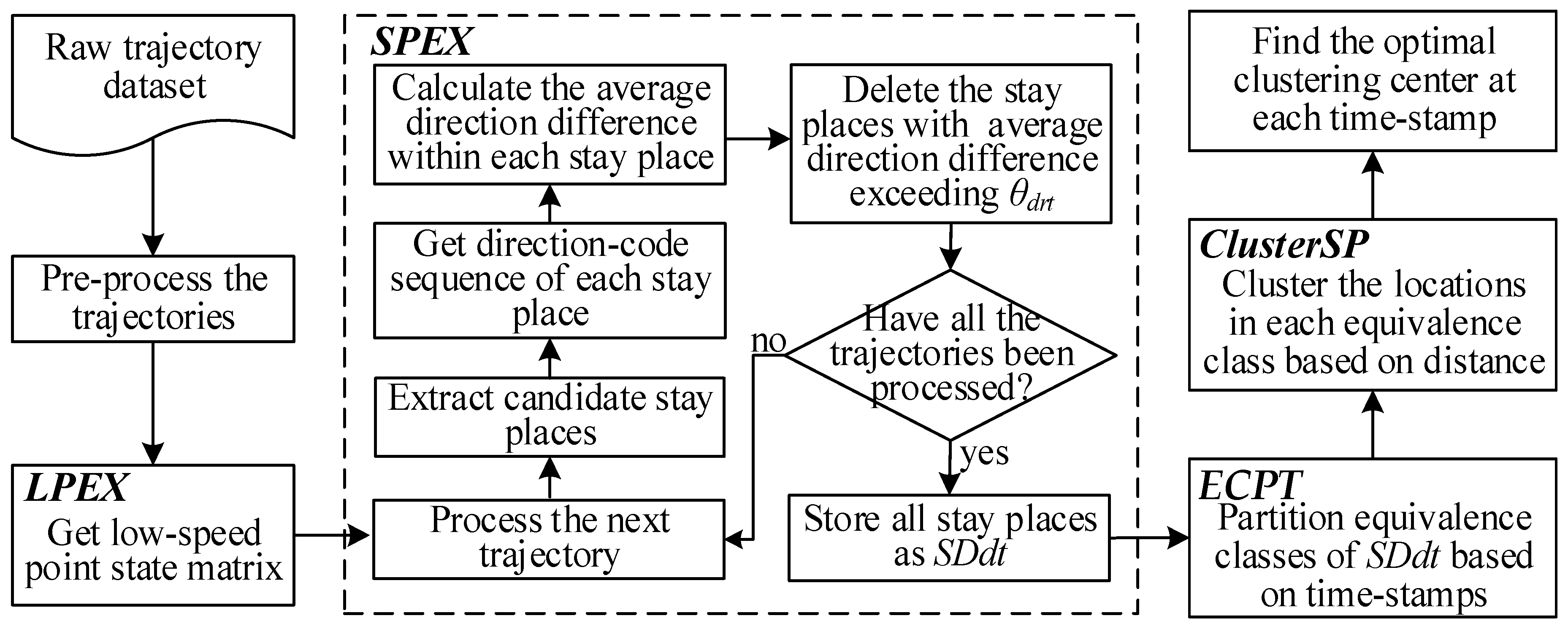
4.1. Algorithm Framework

In this paper, we propose a road congestion location detection approach that helps users effectively avoid the wastage of time caused by congestion during trips. The framework of the proposed approach is shown in Figure 2.

Before mining the trajectory dataset for potential knowledge, it is necessary to pre-process the trajectory dataset. The trajectory pre-processing phase in our algorithm specifically refers to formalization. The trajectory dataset TS is pre-processed so that each $T_i\in TS$ is in the form $T_i=\left\{i, \left(t_1^i,x_1^i,y_1^i\right),\cdots ,\left(t_n^i,x_n^i,y_n^i\right)\right\}$. Each trajectory does not necessarily consist of the same number of time-stamped locations. In the following algorithms, both trajectories and sub-trajectories conform to this form.

The trajectory pre-processing phase is pre-experimental preparation, which is not difficult to achieve. Therefore, the other steps of the detection approach shown in Figure 1 will be focused on. In particular, the proposed congestion location detection approach is denoted as CLDSC, which is implemented by four algorithms. These are LPEX (Low-speed Points Extraction), SPEX (Stay Places Extraction), ECPT (Equivalence Classes Partition), and ClusterSP (Clustering Based on Stay Places), which will be introduced later in Section 4.2, Section 4.3 and Section 4.4.

4.2. Low-Speed Point State Matrix Acquisition

Moving speed is an important indicator that reflects the state of moving objects. If the moving speed at some location is below the designated threshold, it is marked as a low-speed point. The low-speed point state matrix of trajectory dataset TS is acquired by Algorithm 1, denoted as LPEX. The pseudo code of the algorithm is given as follows:

Algorithm 1. LPEX: Low-speed Points Extraction

Input:$TS=\left\{T_1,T_2,\cdots ,T_p\right\}$ (the raw trajectory dataset), ${\theta }_s$ (the speed threshold) Output: LSPS (the low-speed point state matrix) $tn\leftarrow \max \left\{\left|T_1\right|, \left|T_2\right|,\cdots ,\left|T_p\right|\right\};$ Initialize $LSPS\leftarrow zeros\left(p,tn\right)$; fori←1 to pdo  for j←2 to $\left|T_i\right|$ do   if (there is the j-th location in $T_i$) then    $dist\leftarrow \mathrm{Distance}\left(lo{c}_{j-1}^i,lo{c}_j^i\right)$;    $v_{ij}\leftarrow dist/(t_j-t_{j-1})$;    if $(v_{ij}<{\theta }_s)$ then     $LSP{S}_{ij}\leftarrow 1$;    end if   end if  end for end for returnLSPS;

LSPS is a matrix with size $p\times tn$ (Line 2). If the j-th time-stamped location of the i-th trajectory is a low-speed point, its state is set to 1; otherwise, its state is set to 0 (Lines 3–13). The low-speed point state matrix LSPS is the basis of stay places extraction.

The time complexity of Algorithm 1 is O(p$·tn$), which is used to calculate the speed status of each point in each trajectory, where p is the number of trajectories in TS, i.e., p=|TS|, tn is the maximum value of the set $\left\{\left|T_1\right|, \left|T_2\right|,\cdots ,\left|T_p\right|\right\}$, and $\left|T_i\right|$ represents the number of time-stamped locations in $T_i$. The space complexity of Algorithm 1 is also O(p$·tn$), which is mainly caused by storing the matrix LSPS.

4.3. Trajectory Stay Places Extraction Based on Average Direction Difference

4.3.1. Average Direction Difference of Stay Place

In the trajectory of a moving object, there may be different kinds of stay places, as defined in Definition 4. Stay places can be divided into 3 categories: (1) SP I is real stay place. At real stay places, moving objects are doing something meaningful, such as shopping, visiting, eating, etc. This kind of stay place is also regarded as a stay point, which is defined in Definition 5. (2) SP II is signal loss place. The data of certain time-stamped locations in some trajectories are missing because the signal of GPS devices may be blocked by buildings. For these stay places, there may be only a few time-stamped locations for a long period of time. If some data are missing due to poor indoor signals, it is very similar to the first class. (3) SP III is congestion stay place. Congestion stay place refers to the kind of stay place caused by traffic jams. This means that moving objects are waiting at congestion stay places for a long time due to traffic jams. This is a kind of stay place that makes people unhappy. Therefore, detecting congestion stay places plays an important role in the field of traffic management. For example, users can plan better routes to avoid congestion based on the detection results. In this paper, we focus on the third category of stay places. Figure 3 shows a trajectory including the three kinds of stay places, where S₁ and S₂ belong to SP I, S₃ belongs to SP II, and S₄ belongs to SP III.

In Class SP I or SP II area, a user is generally in a purposeful state of staying. As can be seen from the enlarged S₂ at the bottom of Figure 3, the directions of different trajectory segments in such stay places are constantly changing. By contrast, the directions of different trajectory segments are approximately unchanged in the Class SP III area. Therefore, we incorporate the concept of average direction difference into our approach.

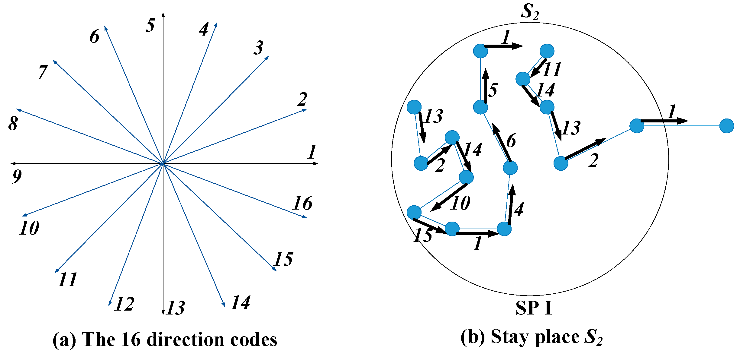
Each trajectory segment has a direction code, which is calculated based on the trajectory direction-code sequence acquisition method proposed in our previous work [29]. At first, the 2D plane coordinate system is evenly divided into N regions according to the angle. Then, a specific direction code is assigned to each region, and the angle of each region is 2·π/N. Let N, the number of direction regions be 16, so the regions with continuous integer codes range from 1 to 16, as shown in Figure 4a. Consider a stay place with SegN trajectory segments. Its average direction difference $Avedd$ is calculated as follows:

$$Avedd=\frac{{{\displaystyle \sum }}_{i=1}^{SegN-1}\min \left\{\left|d{c}_{i+1}-d{c}_i\right|,N-\left|d{c}_{i+1}-d{c}_i\right|\right\}}{SegN-1}$$

(7)

where $SegN$ represents the number of trajectory segments within the stay place, and $d{c}_i$ represents the direction code of the i-th trajectory segment.

For example, Figure 4 displays an example of the direction-code sequence within the stay place S₂ shown in Figure 3. Figure 4a shows the N (=16) direction codes introduced above, and Figure 4b shows the direction codes of different trajectory segments within S₂. More specifically, the direction-code sequence of S₂ is [13,2,14,10,15,1,4,6,5,1,11,14,13,2,1]. The number of trajectory segments segN within this stay place is 15. According to Equation (7), there are 14 (i.e., segN−1) direction difference values that can be calculated for this direction-code sequence. For example, the first one is $\min \left\{\left|d{c}_2-d{c}_1\right|,N-\left|d{c}_2-d{c}_1\right|\right\}$ = $\min \left\{\left|2-13\right|,16-\left|2-13\right|\right\}=\min \left\{11,5\right\}=5$, the second one is $\min \left\{\left|d{c}_3-d{c}_2\right|,N-\left|d{c}_3-d{c}_2\right|\right\}$ = $\min \left\{\left|14-2\right|,16-\left|14-2\right|\right\}=\min \left\{12,4\right\}=4$, the third one is $\min \left\{\left|d{c}_4-d{c}_3\right|,N-\left|d{c}_4-d{c}_3\right|\right\}$ = $\min \left\{\left|10-14\right|,16-\left|10-14\right|\right\}=\min \left\{4,12\right\}=4$, and so on. All the direction difference values are calculated in this way. They are 5, 4, 4, 5, 2, 3, 2, 1, 4, 6, 3, 1, 5, 1. Therefore, its average direction difference value $Avedd=\frac{5+4+4+5+2+3+2+1+4+6+3+1+5+1}{14}=46/14\approx 3.2857$.

In the rest of the article, if not stated, all the stay places we mentioned belong to the third category SP III.

4.3.2. Trajectory Stay Places Extraction

In this section, we introduce the method of trajectory stay place extraction based on the LSPS matrix and average direction difference.

The set of stay places in each trajectory is acquired by Algorithm 2, denoted as SPEX. Consider a trajectory dataset $TS=\left\{T_1,T_2,\cdots ,T_p\right\}$. First, for each trajectory, if at least three consecutive low-speed points meeting the duration requirement are found, they are regarded as one of the candidate stay places in this trajectory. Without loss of generalization, we consider that the trajectory $T_i$ contains sn stay places ($1\le i\le p$), which are successively denoted as $S_1^i,S_2^i,\cdots ,S_{sn}^i$. Each $S_m^i$ ($1\le m\le sn$) contains several low-speed points, which meet the duration requirement (Lines 3–14). Second, the seven-tuples for each stay place $S_m^i$ are calculated (Lines 15–25). The specific meaning of each component in seven-tuple $\langle sn{o}_{S_m^i},en{o}_{S_m^i},s{t}_{S_m^i},e{t}_{S_m^i},x_{S_m^i},y_{S_m^i},d{d}_{S_m^i}\rangle$ (Line 23) can be found in Definition 4.

The pseudo code of the SPEX algorithm is given as follows:

Algorithm 2. SPEX: Stay Places Extraction

Input:$TS=\left\{T_1,T_2,\cdots ,T_p\right\}$ (the trajectory dataset), LSPS (the low-speed point state matrix), ${\theta }_t$ (the time threshold), ${\theta }_{drt}$ (the direction difference threshold) Output: $SDdt$ (the set of stay places in each trajectory) fori ← 1 to p do  k←1; j←1; $S_k^i\leftarrow \varnothing$; $S{D}^i\leftarrow \varnothing$; $SDd{t}^i\leftarrow \varnothing$;  while ($j<\left|T_i\right|$) do   if $LSP{S}_{ij}==0$ then j←j+1; continue; end if   e←j;   while ($LSP{S}_{ie}==1 and e\le \left|T_i\right|$) do    e←e+1;   end while   if (e-j >2 and $lo{c}_{e-1}^i.t-lo{c}_j^i.t>{\theta }_t$) then    $S_k^i\leftarrow S_k^i{\displaystyle \cup }\{lo{c}_j^i,\cdots ,lo{c}_{e-1}^i\}$;    k←k+1; $S_k^i\leftarrow \varnothing$;   end if   j←e;  end while  for m←1 to k−1 do   $sn{o}_{S_m^i}\leftarrow$ the No. of the first location in $S_m^i$;   $en{o}_{S_m^i}\leftarrow$ the No. of the last location in $S_m^i$;   $s{t}_{S_m^i}\leftarrow$ the time stamp of the first location in $S_m^i$;   $e{t}_{S_m^i}\leftarrow$ the time stamp of the last location in $S_m^i$;   $\left(x_{S_m^i},y_{S_m^i}\right)\leftarrow$ the central coordinate of $S_m^i$; // using Equations (2)–(6)   $d{d}_{S_m^i}\leftarrow \mathrm{ComDirectDiff}\left(N,SLdc{s}^i\left(sn{o}_{S_m^i}:en{o}_{S_m^i}-1\right)\right);$   if $(d{d}_{S_m^i}<{\theta }_{drt})$ then    $SDd{t}^i\leftarrow SDd{t}^i{\displaystyle \cup }\left\{\langle sn{o}_{S_m^i},en{o}_{S_m^i},s{t}_{S_m^i},e{t}_{S_m^i},x_{S_m^i},y_{S_m^i},d{d}_{S_m^i}\rangle \right\}$;   end if  end for end for returnSDdt;

In Algorithm 2, the output result is $SDdt=\left\{SDd{t}^1,SDd{t}^2,\cdots ,SDd{t}^p\right\}$, where $SDd{t}^i$ contains all the stay places in the i-th trajectory ($1\le i\le p$).

Note that the central coordinate $\left(x_{S_m^i},y_{S_m^i}\right)$ of $S_m^i$ is calculated using Equations (2)–(6) (Line 20), and $d{d}_{S_m^i}$ is the average direction difference within $S_m^i$ (Line 21), where ComDirectDiff is a function used to measure the amount of change in the direction of trajectory (or sub-trajectory). $SLdc{s}^i$ is a direction-code sequence of the i-th trajectory. In detail, the average value of direction-code differences between each two continuous trajectory segments within a stay place is obtained by calling Function ComDirectDiff, the return value of which is calculated based on Equation (7). Based on the comparison result between $d{d}_{S_m^i}$ and ${\theta }_{drt}$, the final stay places are obtained (Lines 22–24).

The time complexity of Algorithm 2 depends on the following: (a) the time to extract the stay places of each trajectory, whose time complexity is O(p$·tn$); (b) the time to calculate and store the information of each stay place in each trajectory. From Line 21 of Algorithm 2, we know that the direction code sequence of each stay place is scanned to calculate the direction difference using Function ComDirectDiff. Therefore, the time complexity of this part is O(p$·msn·tn$), where $msn$ is the maximum value of the set $\left\{s{n}_1, s{n}_2,\cdots ,s{n}_p\right\}$, and $s{n}_i$ represents the number of stay places in $T_i$. Stay places are derived from time-stamped locations (Lines 3–14), so $msn<tn$. Therefore, the total approximate time complexity of Algorithm 2 is O(p$·t{n}^2$). The space required by Algorithm 2 is p$·msn·7$ because each stay place is recorded using a 7-tuple. Thus, the space complexity of Algorithm 2 is O(p$·msn$), which is mainly from storing the dataset SDdt.

4.4. Congestion Location Detection

4.4.1. Equivalence Classes Partition Based on Timestamps

Road congestion refers to traffic jams caused by a large number of vehicles, disorderly traffic or narrow roads at certain times. The locations visited frequently at different times are not congested locations. Such locations can constitute hot spots. Therefore, to detect road congestion locations, the time attribute must be considered. In this section, the time-stamped locations included in stay places are partitioned according to different timestamp values. For the detection of the same moment, we allow a difference of ${\theta }_t$ seconds before and after, where ${\theta }_t$ is a time threshold. The stay place equivalence class refers to a set consisting of several stay places at approximately the same time.

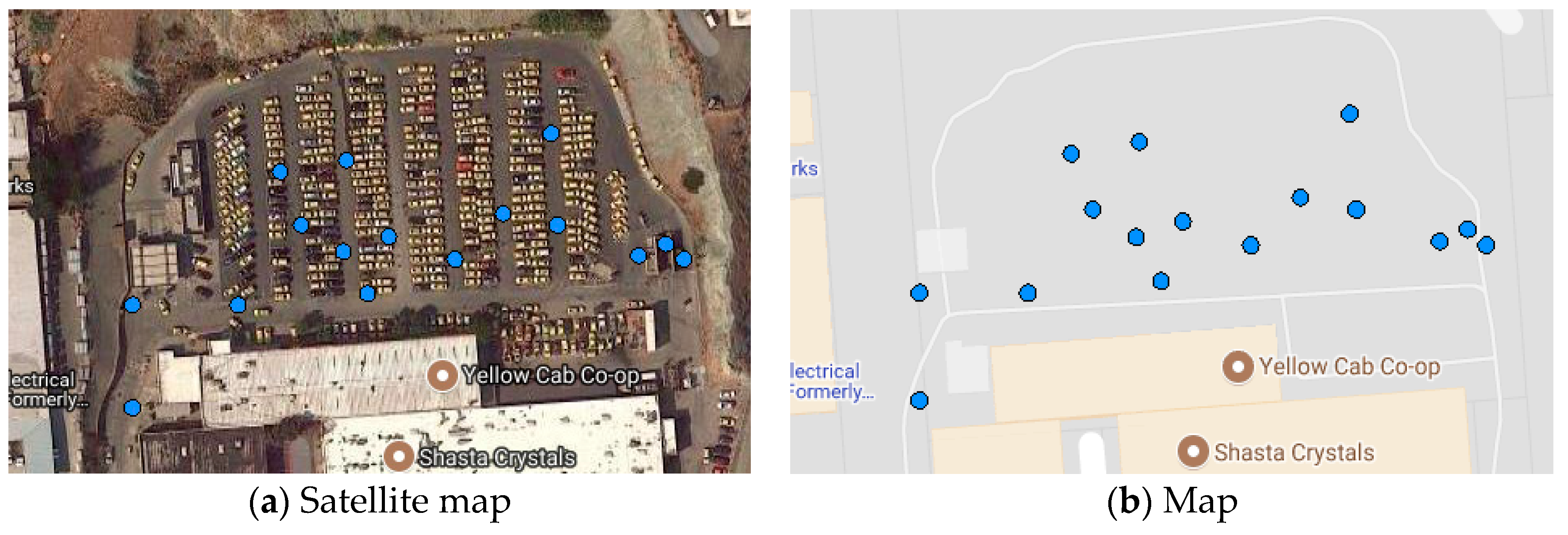
Figure 5 shows the densest area of stay places at 9:18 on 26 May 2008 in San Francisco. The results are detected by our algorithm based on the dataset DS1, which will be introduced in Section 5.2. Each blue point represents a location at that moment. The stay places in similar time periods can reflect that the current locations are in a congested state. Thanks to Bigemap, we can see from Figure 5 that this detected place is the parking lot next to the yellow cab co-op. The day is Monday, and staying in this area at this moment is normal. The detected result is rational and effective.

The set of stay place equivalence classes divided by timestamps is acquired by Algorithm 3, denoted as ECPT. Stay places whose start time and end time meet the specified range requirements are divided into the same equivalence class (Lines 9–13). Different equivalence classes are finally sorted by start time (Line 22).

The pseudo code of the algorithm is given as follows:

Algorithm 3. ECPT: Equivalence Classes Partition

Input:$SDdt$ (the set of stay places in each trajectory), p (the number of trajectories), ${\theta }_t$ (the time threshold) Output: $lscell$ (the set of stay place equivalence classes divided by time) $ln\leftarrow 0$; fori ← 1 to p do  for k←1 to $\left|SDd{t}^i\right|$ do   if ($s{t}_{S_k^i}==-1$) then continue; end if   $ls\leftarrow \left\{\langle s{t}_{S_k^i},e{t}_{S_k^i},x_{S_k^i},y_{S_k^i}\rangle \right\}$;   for j ← 1 to p do    if (j==i) then continue; end if    for q←1 to $\left|SDd{t}^j\right|$ do     if ($\left|s{t}_{S_q^j}-s{t}_{S_k^i}\right|\le {\theta }_t$ and $\left|e{t}_{S_q^j}-e{t}_{S_k^i}\right|\le {\theta }_t$) then      $l\leftarrow \langle s{t}_{S_q^j},e{t}_{S_q^j},x_{S_q^j},y_{S_q^j}\rangle$;      $ls\leftarrow ls{\displaystyle \cup }l$;      $s{t}_{S_q^j}\leftarrow -1$;     end if    end for   end for   $s{t}_{S_k^i}\leftarrow -1$;   $ln\leftarrow ln+1$;   $lscel{l}^{ln}\leftarrow ls$;  end for end for $lscell\leftarrow \left\{lscel{l}^1,lscel{l}^2,\cdots ,lscel{l}^{ln}\right\}$; Sort $lscell$ in ascending order by the start time; return$lscell$;

The start and end time of each stay place of each trajectory are compared with those of all the other stay places. The stay places with similar start and end times are partitioned into the same equivalence class (Lines 2–20). Therefore, the time complexity of Algorithm 3 is O($totals{n}^2$), where $totalsn$ represents the total number of stay places within the trajectory dataset.

4.4.2. Stay Places Clustering Based on Equivalence Classes

Existing methods mainly concentrate on the analysis of separated congestion locations and cannot provide time-ordered congestion sequence in periodic motions. Therefore, after the set of stay place equivalence classes divided by timestamps is obtained, we cluster stay places in each stay place equivalence class according to their central coordinates, to mine the aggregation locations of multiple trajectories during a certain period of time. The clustering process is implemented by Algorithm 4, denoted as ClusterSP. After this algorithm is executed, all the cluster centers and the optimal cluster center of each equivalence class are acquired, and the set of time and central coordinates of stay places belonging to the optimal cluster in each equivalence class is also obtained to be displayed visually on a real map. The notations used in the ClusterSP algorithm are listed in

Table 1. Notations used in ClusterSP algorithm.

Notation	Description
$Idxcel{l}^i$	The set of cluster labels in the i-th equivalence class
$Ccel{l}^i$	The set of cluster centers in the i-th equivalence class
$sumDcel{l}^i$	The set of the sum of distances between each point and its center within each cluster in the i-th equivalence class
$lscel{l}^i$	The set of stay places in the i-th equivalence class
$ECt{s}^i$	The two-tuple <start time, end time> in the i-th equivalence class
$ECloc{s}^i$	The set of the central coordinates of each stay place in the i-th equivalence class
$ECcl{s}^i$	The number of clusters in the i-th equivalence class

.

The pseudo code of ClusterSP algorithm is given as follows:

Algorithm 4. ClusterSP: Clustering Based on Stay Places

Input:$lscell$ (the set of stay place equivalence classes divided by time), K (the number of clusters) Output: Ccell (the set of cluster centers in each equivalence class), BestC (the set of optimal cluster centers in each equivalence class), OriBestLocs (the set of time and central coordinates of stay places belonging to BestC), eqs ← the number of equivalence classes in $lscell$; fori ← 1 to eqs do  $ECt{s}^i$ ← time data from Row 1 and Columns 1–2 of the matrix $lscel{l}^i$;  $ECloc{s}^i$ ← location data from Columns 3–4 of the matrix $lscel{l}^i$;  [Idx, C, sumD] ← kmeans ($ECloc{s}^i$, K);  $Idxcel{l}^i$ ← Idx;  $Ccel{l}^i$ ← C;  $sumDcel{l}^i$ ← sumD; end for $Ccell\leftarrow \left\{Ccel{l}^1,Ccel{l}^2 ,\cdots ,Ccel{l}^{eqs} \right\}$; OriBestLocs ← $\varnothing$; fori ← 1 to eqs do $ECcl{s}^i$ ← the number of clusters in $ECloc{s}^i$;  if $(ECcl{s}^i==1)$ then   $Best{C}^i$ ← <$ECt{s}^i, Ccel{l}^i$>;   OriBestLocs ←OriBestLocs ${\displaystyle \cup }lscel{l}^i$;  else   Minavg ← Inf; jmin ← −1;   for j ← 1 to $ECcl{s}^i$ do    num ← the number of locations in the j-th cluster of $Idxcel{l}^i$;    avg ← $sumDcel{l}^i\left(j\right)/num$;    if (avg < Minavg) then     Minavg ← avg; jmin ← j;    end if   end for   $bloc{s}^i$ ← the jmin-th center in $Ccel{l}^i$;   $Best{C}^i$ ← <$ECt{s}^i, bloc{s}^i$>;   xh ← find ($Idxcel{l}^i$==jmin);   OriBestLocs ←OriBestLocs ${\displaystyle \cup }lscel{l}^i\left(xh,:\right)$;  end if end for $BestC\leftarrow \left\{Best{C}^1,Best{C}^2 ,\cdots ,Best{C}^{eqs} \right\}$; returnCcell, BestC, OriBestLocs;

Lines 1–9 complete the process of clustering based on stay places in each equivalence class, where “kmeans” in Line 5 is a Matlab function used to implement k-means clustering. In the experiments, the parameter K is set as $\left|lscel{l}^i\right|/3$ for the i-th stay place equivalence class $lscel{l}^i$. This is set according to the number of stay places within each equivalence class. The experimental results on the four trajectory datasets (which will be introduced in Section 5.2) show that the maximum number of stay places in $lscell$ is 31. Lines 10–31 get the set of optimal cluster centers in each equivalence class and the set of time and central coordinates of stay places belonging to optimal clusters, where ($Idxcel{l}^i$==j_min) in Line 28 is a Matlab function used to find the indexes of the elements with value j_min in $Idxcel{l}^i$, and $lscel{l}^i\left(xh,:\right)$ in Line 29 represents the data of all rows whose row numbers belong to the vector xh.

The time complexity of Algorithm 4 depends on the following: (a) the time taken for clustering within each equivalence class, whose time complexity is O(eqs$·$Tkmeans), where Tkmeans is the number of iterations in k-means clustering; (b) the time taken to calculate the optimal cluster centers, whose time complexity is O(eqs$·$mECcls), where mECcls represents the maximum value of the set $\left\{ECcl{s}^1,ECcl{s}^2,\cdots ,ECcl{s}^{eqs}\right\}$.

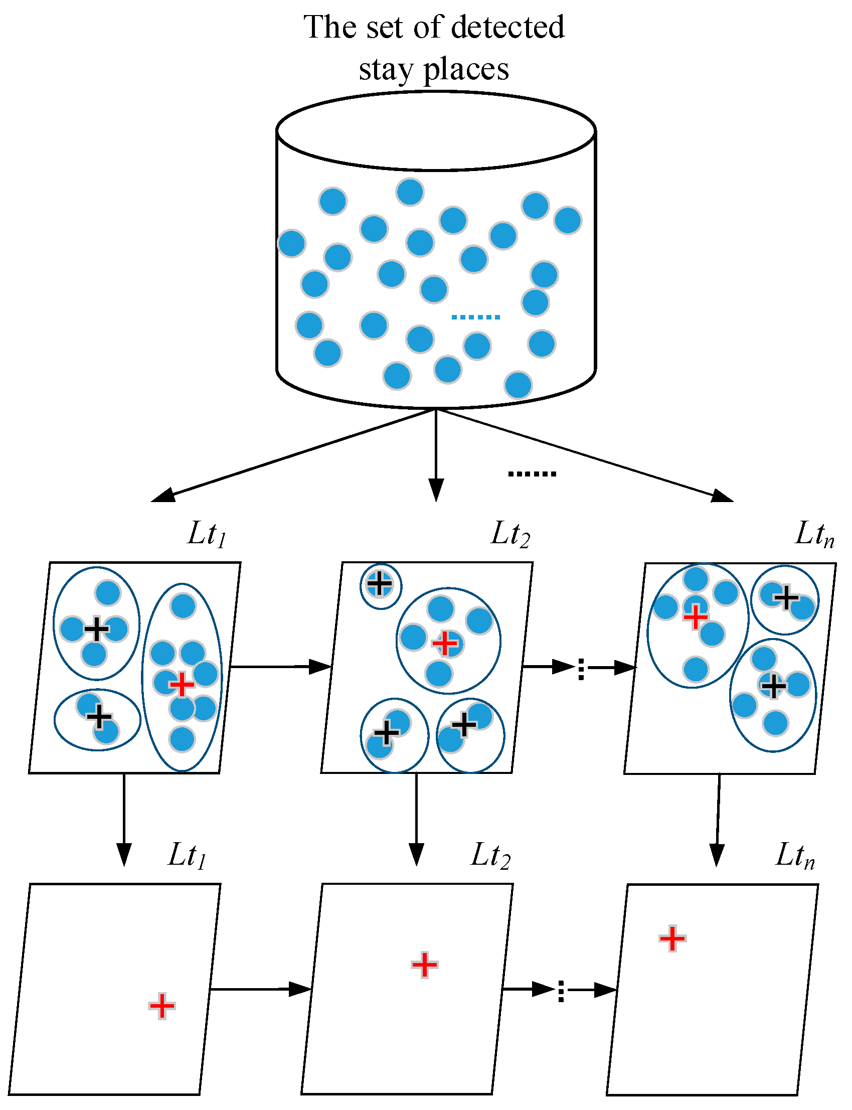
Figure 6 shows the hierarchical graph of optimal stay-place sequence detection based on the proposed approach. In Figure 6, the symbol Lt_i represents the set of stay places in the i-th time period ($1\le i\le n$). (1) The top layer is the set of detected stay places SDdt extracted using Algorithm 2. (2) The middle layer contains several sets of stay places in different time periods, which are stored in the set of stay place equivalence classes $lscell$ acquired by Algorithm 3. In each equivalence class of $lscell$, stay places are clustered according to their central coordinates. The clustering process is implemented by Algorithm 4. (3) The bottom layer shows the sequence of optimal stay places obtained based on the clustering results within different equivalence classes.

5. Experiments

In this section, we perform a set of experiments to evaluate the performances of the proposed algorithms. We first present the experimental settings which consist of the introduction to the experimental environment, and some parameters we selected for the experiments. Then, the datasets and evaluation metrics used in the experiments are introduced. Finally, the visualization of the experimental results is shown, and the proposed approach is evaluated in terms of average precision, average recall, average F and average MissRate.

5.1. Experimental Environment and Parameter Selection

The experiments are conducted with Matlab 8.3 on a PC with Intel (R) Core (TM) 2 Duo CPU 3.7 GHz and 8 GB of RAM. The operating system is Microsoft Windows 7. A real-life dataset is used to conduct our experiments.

According to Algorithms 1–4, our experimental process is specifically arranged as follows: (1) Pre-process the experimental datasets based on the proposed trajectory model. (2) Extract the low-speed points and stay places using Algorithm 1 and Algorithm 2, respectively. (3) Conduct equivalence class partitioning using Algorithm 3. (4) Detect the road congestion locations based on Algorithm 4. (5) Experimental results and related analysis.

The parameters used in Algorithms 1–4 include the speed threshold ${\theta }_s$, the time threshold ${\theta }_t$, and the direction difference threshold ${\theta }_{drt}$. They are set specifically according to the related experimental results, which will be described later.

5.2. Dataset

The real-life dataset of cab moving trajectories collected from San Francisco in the United States [30,31] is used in our experiments. It contains GPS coordinates of approximately 500 cabs in the San Francisco Bay Area from May to June 2008. The locations in this dataset are very fine-grained because the average time interval between two consecutive locations is less than 10 s [31]. The format of each mobility trajectory file is as follows: each line contains latitude, longitude, occupancy, and time, where the occupancy is ignored in our experiments. As the trajectory of a cab over the course of an entire month can hardly be considered a single trajectory, we use the method in literature [7] to pre-process this dataset. In particular, the trajectory data between 25 May at 12:04 and 26 May at 12:04 is extracted by referring to Literature [7]. This dataset has a high concentration of locations. After a trajectory filtering process, we obtain 481 trajectories and 896 locations per trajectory on average. The longest trajectory contains 2483 locations. For ease of description, this dataset is denoted as DS1.

For contrast, the other three datasets are extracted from the real-life taxis trajectory dataset. These four datasets are extracted from the same time period of four consecutive weeks. Specifically, (1) the trajectory data between 18 May at 12:04 and 19 May at 12:04 is extracted as dataset DS2, which includes 492 trajectories and 967 locations per trajectory on average. The longest trajectory contains 2119 locations; (2) the trajectory data between 1 June at 12:04 and 2 June at 12:04 is extracted as dataset DS3, which includes 491 trajectories and 923 locations per trajectory on average. The longest trajectory contains 2030 locations; (3) the trajectory data between 8 June at 12:04 and 9 June at 12:04 is extracted as dataset DS4, which includes 499 trajectories and 883 locations per trajectory on average. The longest trajectory contains 2411 locations. The common characteristics of these four datasets are that they all record trajectories from 12:04 on Sunday to 12:04 on Monday.

5.3. Evaluation Metrics

Based on the reference stay points detected by the StayPointDetection algorithm [14,32], we evaluate the performance of the proposed approach in terms of the following statistical metrics [17,33]:

(1) Precision: the ratio between the number of correctly detected stay locations and the number of all the detected stay locations:

$$Precision=\frac{TP}{TP+FP}$$

(8)

where TP (True Positive) represents the number of stay locations being truly detected, and FP (False Positive) represents the number of moving points being falsely detected as stay locations.

(2) Recall: the ratio between the number of correctly detected stay locations and the number of the actual stay locations.

$$Recall=\frac{TP}{TP+FN}$$

(9)

where FN (False Negative) represents the number of stay locations being falsely detected as moving ones.

(3) F measure: the weighted harmonic mean of precision and recall.

$$F=\frac{2\times Precision\times Recall}{Precision+Recall}.$$

(10)

The range of F value is [0,1]. A higher value means that the algorithm has better performance.

(4) MissRate: the ratio between the number of undetected stay locations and the number of reference stay locations.

$$MissRate=\frac{FN}{TP+FN}.$$

(11)

In fact, the sum of Recall and MissRate is 1. The higher the Recall value, or the lower the MissRate value, the better the performance of the algorithm.

The values of the above metrics are calculated for each trajectory in the dataset. Therefore, for the whole trajectory dataset, the average values of each metric are adopted to evaluate the detection performance of our approach.

5.4. Experimental Results

In this section, both the experimental results and related analysis are given. A set of comparative experiments are firstly conducted to evaluate the performance of the proposed approach. Then, the detected congestion locations are visually displayed.

5.4.1. Detection Accuracy of Stay Points

We use the four metrics mentioned in Section 5.3 to evaluate the detection accuracy of stay points. To better illustrate the extraction results of trajectory stay points, we change the values of the corresponding parameters in the algorithms.

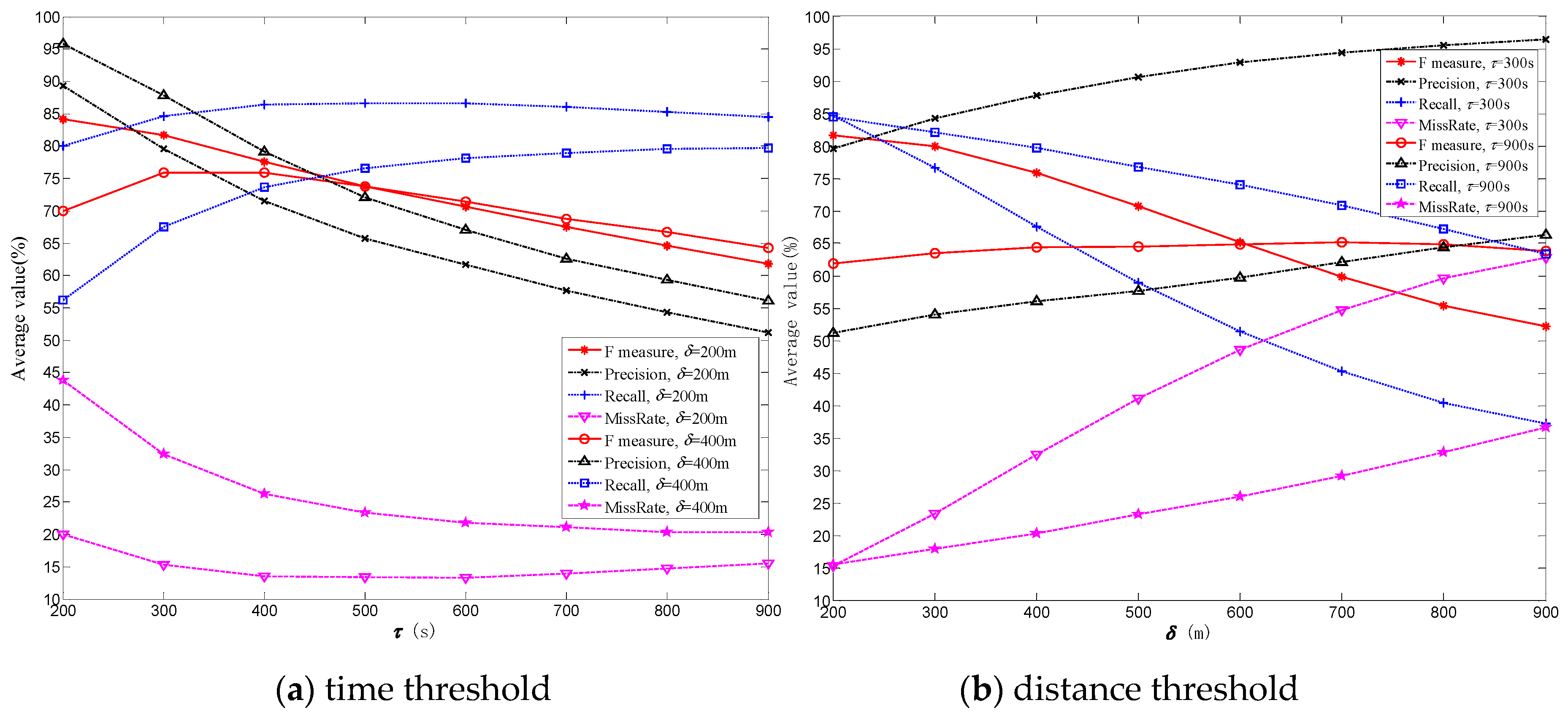
The stay points detected by the StayPointDetection algorithm [14,32] are used as a reference to verify the detection accuracy of our algorithms. The original time-stamped locations contained in the stay places detected by Algorithms 1 and 2 (LPEX and SPEX) are compared with the reference stay points. The extraction of stay places is the basis of our congestion detection approach. It is important to verify the accuracy of the extraction results.

On one hand, we change the values of parameters $\tau$ and $\delta$ in the StayPointDetection algorithm, where $\tau$ is the stay time threshold, and $\delta$ is the distance threshold. According to the literature [14], the distance threshold $\delta$ is set to 200 meters, and the stay time threshold $\tau$ is set to 15 minutes. We vary $\tau$ from 200 s to 900 s, and vary $\delta$ from 200 m to 900 m. In our proposed method, ${\theta }_t$ is set to 100 s, ${\theta }_s$ is set to 2.22 m/s, and ${\theta }_{drt}$ is set to 7. Figure 7 shows the comparison results of F, Precision, Recall, and MissRate values based on the change of parameters in the StayPointDetection algorithm. In Figure 7a, $\delta$ is set to 200 m or 400 m, and the average values of all trajectories in DS1 for each metric are calculated in the case of different $\tau$ values. In Figure 7b, $\tau$ is set to 300 s or 900 s, and the average values of all trajectories in DS1 for each metric are calculated in the case of different $\delta$ values.

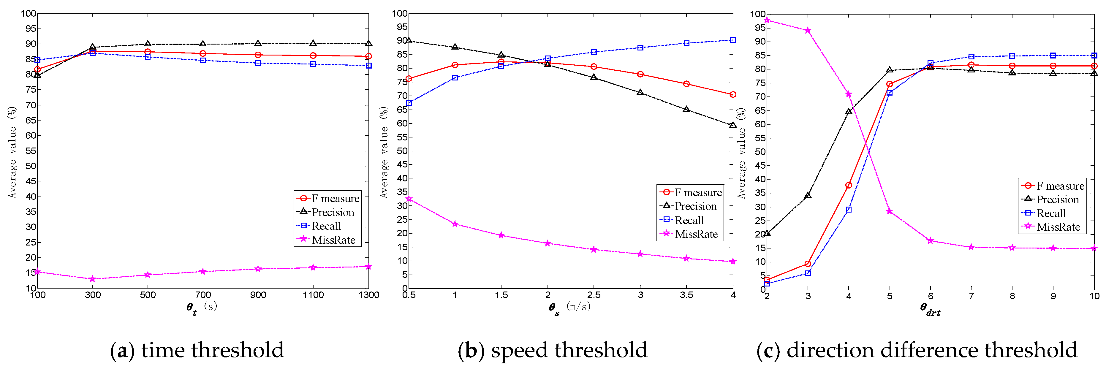
Meanwhile, we change the values of parameters ${\theta }_t$, ${\theta }_s$, and ${\theta }_{drt}$ in our algorithms. Specifically, we vary ${\theta }_t$ from 100 s to 1300 s, vary ${\theta }_s$ from 0.5 m/s to 4 m/s and vary ${\theta }_{drt}$ from 2 to 10. In StayPointDetection algorithm, $\delta$ is set to 200 m, $\tau$ is set to 300 s. Figure 8 shows the comparison results of F, Precision, Recall, and MissRate values based on the change of parameters in the LPEX and SPEX algorithms. In Figure 8a, the average values of all trajectories in DS1 for each metric are calculated in the case of different ${\theta }_t$ values. In Figure 8b, the average values for each metric are calculated in the case of different ${\theta }_s$ values. In Figure 8c, the average values for each metric are calculated in the case of different ${\theta }_{drt}$ values.

As can be seen from Figure 7 and Figure 8, the locations within stay places detected by our algorithm have a high accuracy when referring to the results of the Algorithm StayPointDetection based on dataset DS1. The average values of F measure are more than 80% under specified parameters. This means that the stay places extracted by our method contain most of the stay points detected by the classic stay point detection algorithm StayPointDetection; the main difference is because of the deletion of stay places that exceed ${\theta }_{drt}$. Note that the purpose of the two algorithms is not the same. StayPointDetection algorithm is used to detect the stay points that meet the specified time and distance requirement. The proposed algorithm SPEX is used to extract the stay places within which there is no large direction difference between different trajectory segments. Therefore, the detection results have some missing data when compared with reference results, which are reflected by the average Recall value and the average MissRate value. As shown in Figure 8c, the average F value increases as ${\theta }_{drt}$ increases, and the F value is substantially stable when ${\theta }_{drt}$ reaches 7. The smaller ${\theta }_{drt}$ is, the more candidate stay places will be deleted, so the F value will be smaller, and vice versa. However, if ${\theta }_{drt}$ value is too large, the detected stay places most likely belong to the category of SP I instead of SP III. Therefore, we set ${\theta }_{drt}$ to 7 in the experiments.

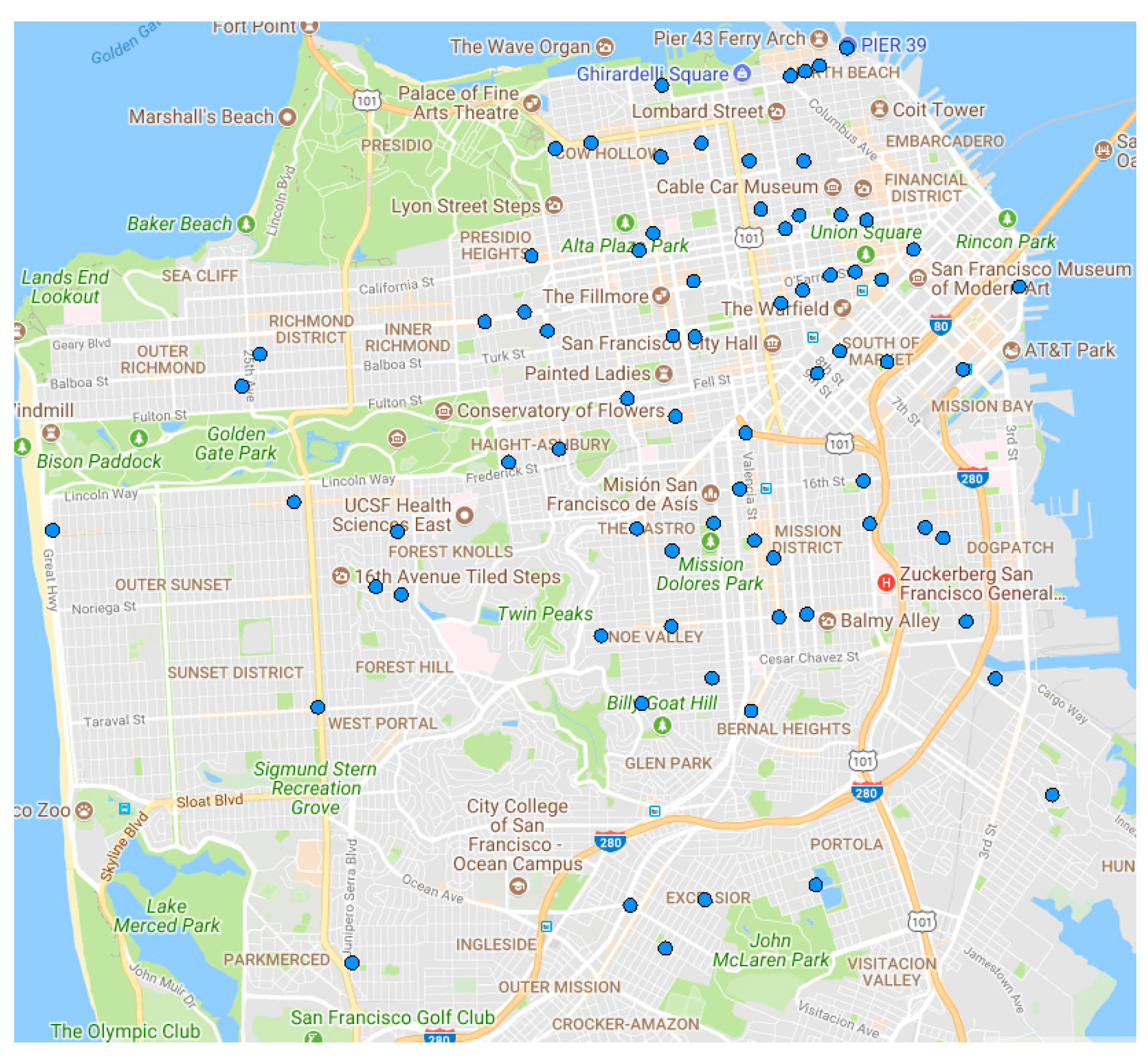
5.4.2. Visual Display of the Detection Results

Using our approach, the optimal cluster centers of each equivalence class are obtained. Based on the detection results on DS1 dataset, the most densely distributed areas of congestion are represented in Figure 9. This area mainly concentrates in the northeast part of San Francisco, which is a relatively populous area.

Congestion locations are of two types: recurrent ones and non-recurrent ones. The main difference between the two is whether the congestion event at the congestion location is accidental or recurring at a given time. Therefore, the detection of recurrent congestion relies on experiments using datasets with periodic time periods. Next, we use four datasets, DS1–DS4, from the same time period for the experiments on congestion location detection and visualize the results.

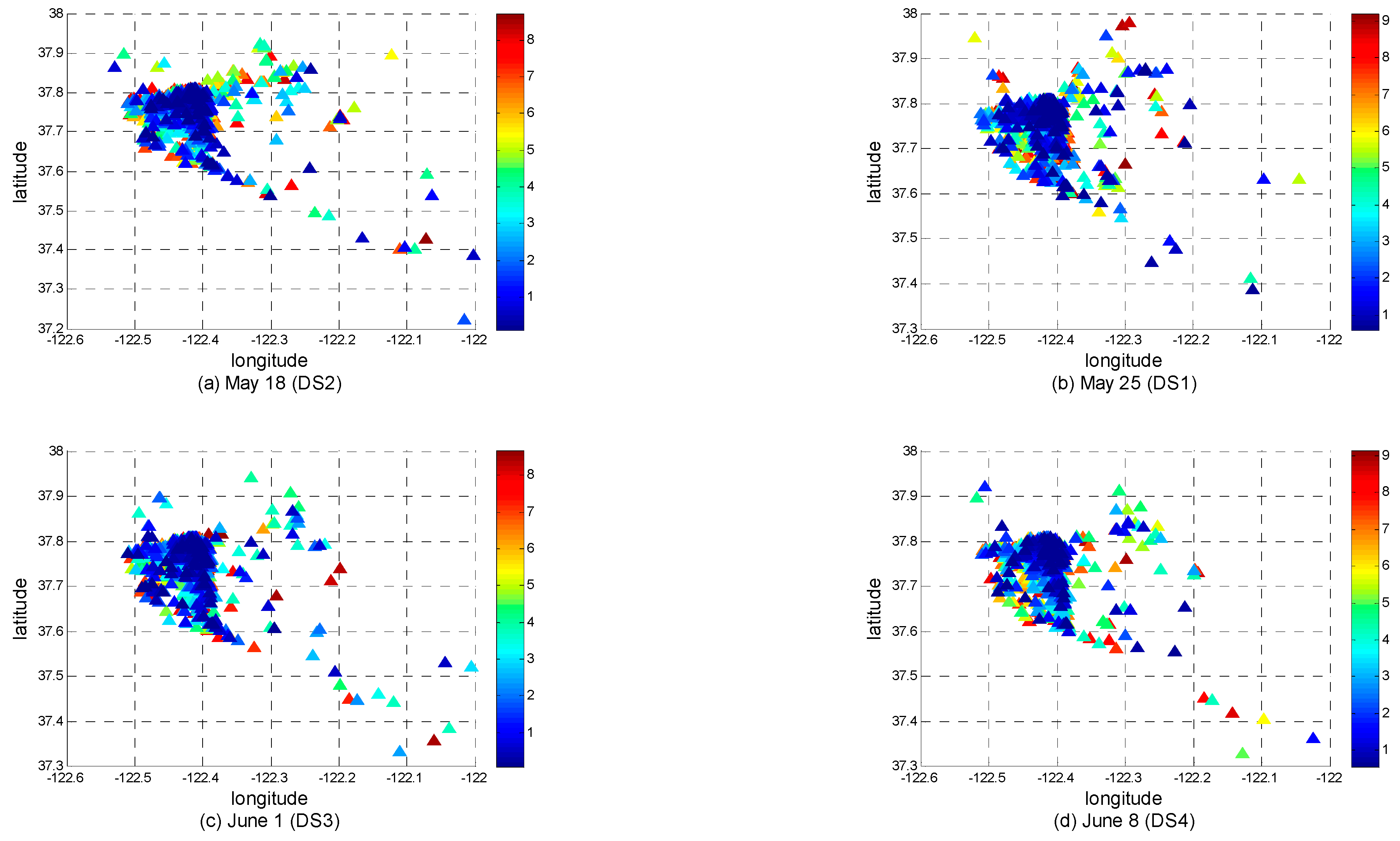
To facilitate the display of the optimal centers of stay places at different timestamps, we color them in chronological order. The coloring graphs on datasets DS1–DS4 are shown in Figure 10. The clustering method is k-means.

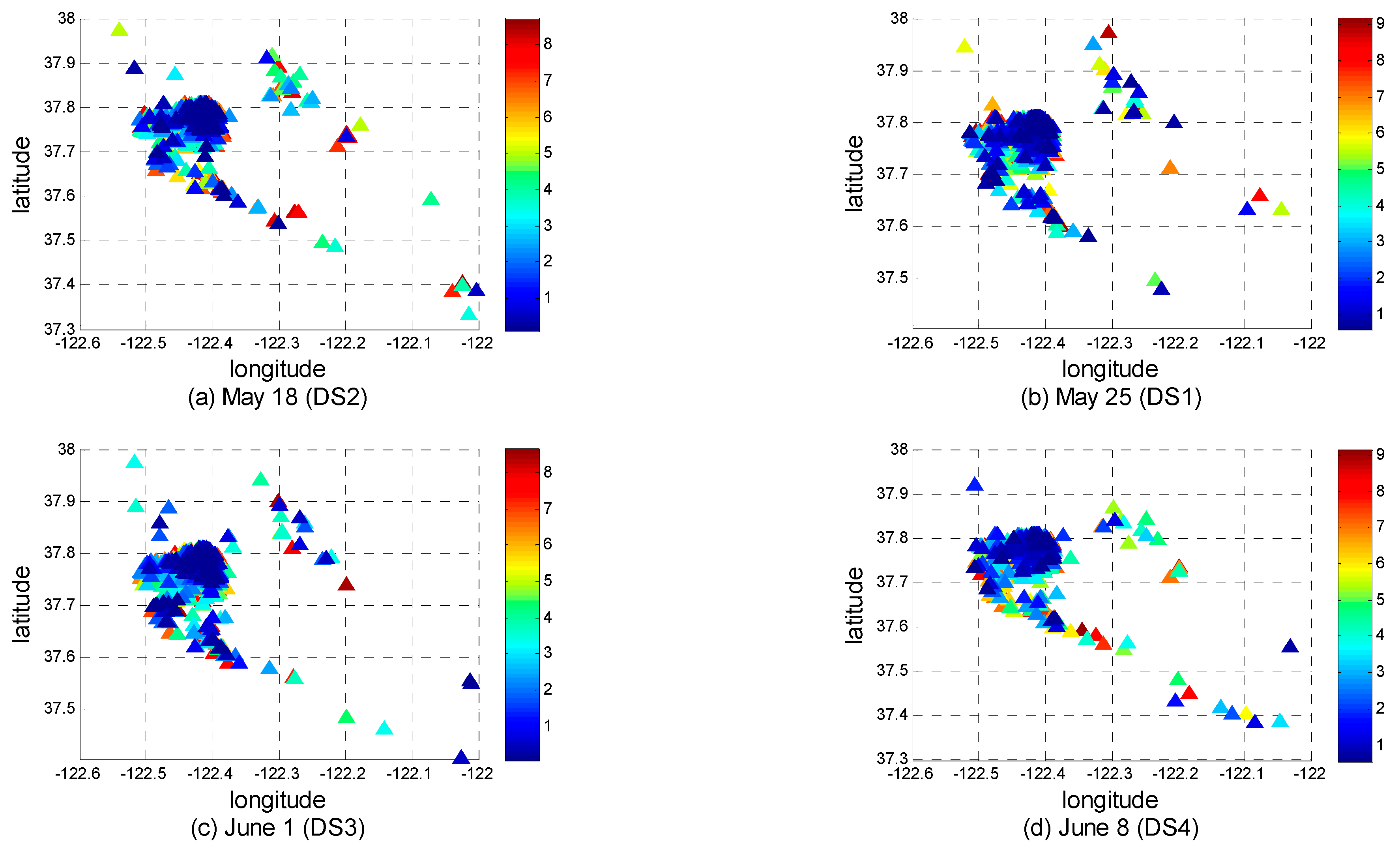
As a comparison, the clustering method of DBSCAN (Density-Based Spatial Clustering of Applications with Noise) is also used to conduct the same experiments. Figure 11 shows the corresponding running results.

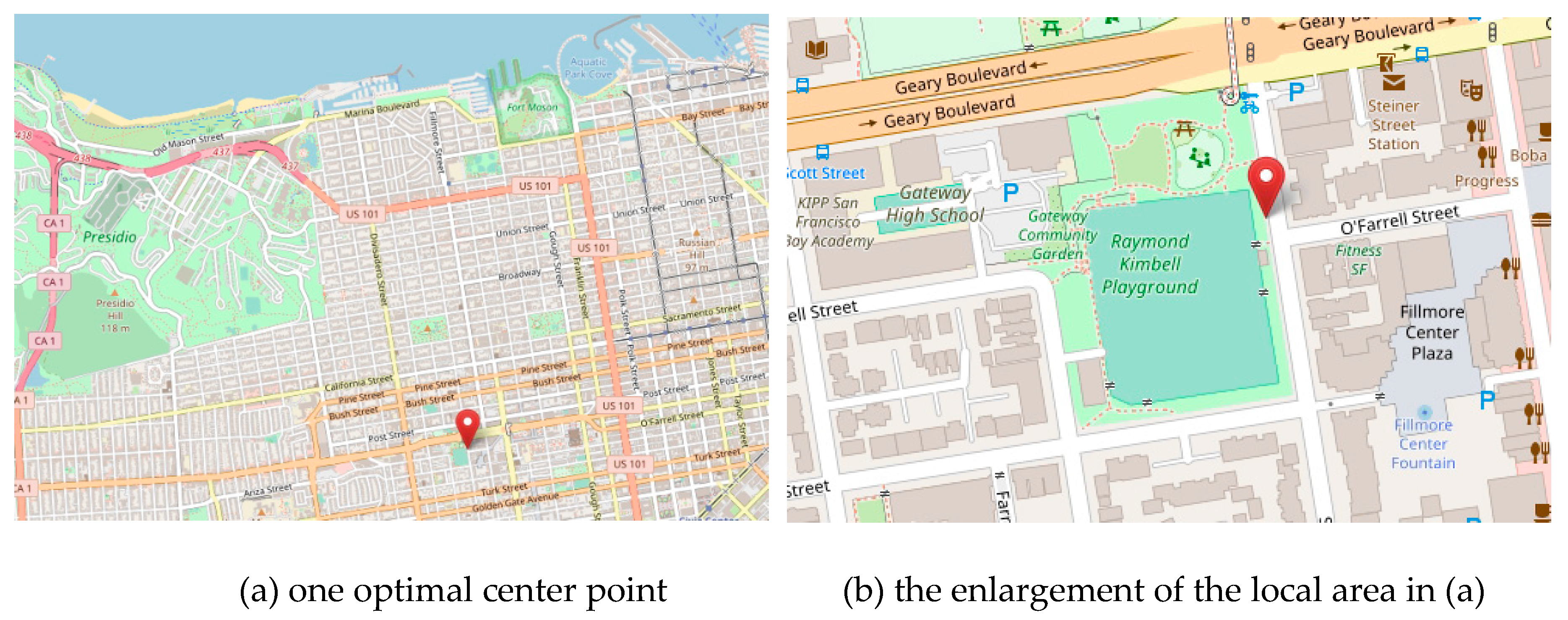
As can be seen from Figure 10 and Figure 11, every Monday, taxis in San Francisco appear more concentrated in the latitude and longitude range (37.7, −122.45, 37.8, −122.4). The results of the two clustering methods are similar in this respect. Just as with the distribution shown in Figure 9, this area is located in the northeast of San Francisco. Take one optimal center point in the running result of Figure 10a as an example. The time and location information of the optimal stay center is (1211745933, 1211747557, 37.7832, −122.4345), where the first two numbers are, respectively, the start time and end time of this stay center recorded with the Unix timestamps. After the Unix timestamps are converted to ordinary date and time, the start and end times of this stay place are 13:05:33 and 13:32:37 on 25 May 2008, respectively. The center of this stay place is close to Raymond Kimbell Playground, which is shown in Figure 12. From these detection results, we can identify recurrent congestion locations.

In summary, the centers of congestion locations at different timestamps are obtained based on the detection results, which can be used as a guide for transportation supervision and personal travel route planning in San Francisco.

6. Conclusions

In this paper, we propose a novel approach for detecting road congestion locations based on trajectory stay-place clustering. Before the execution of our algorithms, a trajectory dataset is pre-processed according to Definition 1. There are four steps in this approach. First, the speed status of each point in each trajectory is calculated for obtaining the low-speed point state matrix. Second, the trajectory stay places extraction is implemented based on average direction difference. Third, the time-stamped locations included in the stay places are partitioned into different stay-place equivalence classes according to different timestamps. Finally, we cluster stay places in each equivalence class according to their central coordinates, to mine the aggregation locations of multiple trajectories during a certain period of time. Visual representations and simulated experimental results on real-life cab trajectory datasets show that the proposed approach can obtain effective and reasonable congestion clusters for vehicles data and provide worthwhile services for traffic periodic management system. This achievement is convenient enough to be applied in road planning and may be used in the aggregation analysis of other moving objects in the city. In future research, we plan to integrate the features of POI (Point of Interest) near the road, the drivers’ travel purposes, and behavior features to mine deep causation of congestion formation and conduct travel recommendations.