1. Introduction
Cartographic generalization is the process of generating smaller scale representations from large scale spatial data. This process is being conducted by cartographers by applying different operators, such as selection, simplification or displacement, which—in sum—lead to a simpler and a more clear representation of the spatial scene at a smaller scale. There are many powerful automatic solutions for individual operators. The main challenge today lies in mastering the interplay between different operators, for which e.g., optimization approaches, rule based approaches, or agent based approaches are used. Here, however, the benchmark is still the human operator, who is able to design an aesthetic and correct representation of the physical reality by a careful orchestration of several operators.
Deep learning methods have shown impressive success for interpretation problems for which algorithmic methods are difficult. A prominent example is the classification and interpretation of images, where deep learning approaches outperform traditional computer vision methods. In both domains-computer vision and cartography-humans are very well able to produce good solutions. Hence, the idea in this paper is to employ deep convolutional neural networks (DCNNs) for cartographic generalizations tasks, especially for the task of building generalization. Many deep learning approaches are based on supervised learning, i.e., they require example data with given input–output pairs. Fortunately, in map generalization, many training data sets are available from the existing map series.
Thus, the idea is straightforward to utilize the deep learning approaches on rasterized building maps for the generalization problem. The neural network architectures applied in this paper are similar to the models used for semantic segmentation [
1]. These methods do not provide one classification for a given image patch, but lead to a classification of each pixel. Thus, the output is again an image, however with a label for each pixel. In this paper we adopt this idea. In our case, both the input and output are binary raster images.
The paper presents initial experiences with a straightforward implementation and adaption of some of the well-known existing network architectures, namely U-net, residual U-net and generative adversarial network (GAN). The goal is to explore the potential of deep learning for a cartographic problem.
This paper is organized as follows. The next section is a summary of the state-of-the-art approaches for cartographic generalization. Related works regarding deep neural networks are introduced. In
Section 3, the details of the data preparation, implementation and training the models will be reported. In
Section 4, an in-depth analysis and discussion of the results will be given both quantitatively and qualitatively. In the last section, we conclude and give an outlook on future work.
2. State of the Art
The automation of building map generalization has been studied by many researchers in recent years—mainly coming from cartography, geoinformatics, and computer science, especially computational geometry (e.g., [
2]). The methods are often based on geometric considerations; the integration of operators is relying on optimization (e.g., [
3]), rule sets (e.g., [
4]), or agent based methods (e.g., [
5]).
The approaches are being mainly applied in vector space, however, there are also methods using rasterized representations of the spatial scene. Examples for this kind of operations are aggregation, typification (e.g., [
6]), displacement (e.g., [
7]), and also building generalization (e.g., [
8,
9]). A recent approach [
10] has applied superpixel segmentation and clustering to simplify and aggregate polygonal features.
Building generalization involves different elements, such as selection (according to size, type or usage), aggregation (in order to close small gaps) and simplification of the building outline. During this process, the typical shape of a building has to be preserved or even enhanced. This often involves rectifying nearly right angles and enforcing parallel lines in the building footprint, which, for instance, can be achieved using a set of rules (e.g., [
3,
11]). The factors controlling the generalization depend on the scale, and the area of the building, as well as small structures (facade lengths). When moving to even smaller scales, these parameters would lead to an elimination of most of the buildings, therefore, then typification is applied, i.e., the replacement of the buildings by a building template (mostly square or rectangle) while preserving their spatial arrangement. This operation is applied at scales 1:40,000 and smaller.
There have been early attempts to use machine learning to extract cartographic rules from given examples. One goal was to learn suitable parameters of operations (e.g., [
12]). In their work, the authors observed a human cartographer in order to learn his actions. In a similar way, Mustière [
13] aimed at identifying optimal sequences of operators using machine learning. Sester [
14] tried to extract spatial knowledge from given spatial data. While these approaches were very interesting, they mainly remained proofs of concepts.
Deep learning as a new paradigm has re-emerged in recent years, triggered by the now available computational power (especially exploiting GPUs)—allowing us to also design very deep (many layers) and complex networks—and large quantities of available training data. The success in image interpretation was much influenced by the development of new modelling schemes like CNN [
15]. They constrain the number of connections in the network to local environments, thus mimicking the human visual system with it perceptual fields, but also constraining the relations of neurons based on neighborhood principles. Such models have been applied in many different disciplines to classify images, e.g., digit or characters recognition (e.g., [
16]), information retrieval of certain scenes (e.g., [
17,
18]). In further, the fully convolutional networks [
19] and its subsequent network architectures achieved to assign class label to each pixel—which is called semantic segmentation. Such methods are being applied in very relevant tasks such as intelligent security systems, autonomous driving and health-care, as well as in topographic mapping, such as semantic segmentation of aerial images (e.g., [
20,
21]), road extraction from remote sensing images [
22].
In the generalization domain, recently machine learning has been proposed for different applications. Xu et al. [
23] used an deep autoencoder network to asses the quality of building footprint data by learning the characteristics of quality from OpenStreetMap (OSM) and authoritative data. Zhou and Li [
24] compared different machine learning approaches concerning their capability to select important road links for road network generalization. Lee et al. [
25] used different machine learning methods to classify buildings as a prior step for their generalization. Cheng et al. [
26] propose a Neural Network to detect and learn local situations in building ground plans, which have to be replaced by simpler situations. An approach for generalization of lines from traffic trajectories using deep learning has been proposed by Thiemann et al. [
27].
To the best of our knowledge, the approaches proposed in this paper are the first attempts to develop end-to-end solutions for cartographic building generalization using DCNNs. The models do not only learn the simplification of building outlines, but also the aggregation and selection of buildings in one model at the same time. This is an advantage as opposed to most existing solution, which are often focusing on the automation of ONE operation (e.g., simplification of outline); other approaches need dedicated, explicit interaction rules to describe the interplay between different operations (e.g., agent based approaches). Our models do not learn the choice of operations e.g., elimination, simplification, or aggregation as in [
25], but generate the generalization results directly, so that the interplay between operators does not need to be considered.
3. Approach
Building generalization is composed of different sub-processes: small buildings are eliminated (selection), small parts of the building outline are eliminated, the outline is simplified (simplification), neighboring objects can be merged (aggregation), too-small buildings can be enlarged (enhancement), buildings are displaced (displacement) and finally, groups of buildings may be replaced by another group, however, with less objects (typification) [
28]. The approach presented in this paper aims at an end-to-end training scheme, where an input and a target output are given, and the system has to learn the operations in between. Thus, the expectation is that the system learns all these generalization operations in a holistic way.
In order to train the neural networks, examples have to be provided in terms of corresponding input and output data-pairs. Those data sets are available from existing maps, where situations before and after generalization are depicted. In our approach, we rely on an image based approach, which means that the data is prepared in terms of raster images. One straightforward option would be to use image patches around individual buildings as training data; however, we decided to use the whole map as such, which is cut into regular image patches of given size b × b. When selecting an appropriate size for b, this approach ensures, that adequate context around each building is implicitly used.
In this paper, three network architectures are applied for building generalization. This is a substantial extension of a previous work [
29], where only one architecture was employed. The idea of that paper was inspired by the work from Simo-Serra [
30], where sketch drawings were simplified using a deep convolutional neural network. In another attempt of generalization using deep learning, a similar deep neural network structure has been applied to the problem data aggregation, namely to extract a road map from car trajectories [
27].
The models evaluated in this paper originate from algorithms used in computer vision, namely U-net [
31], residual U-net [
32] and GAN [
33]. Some modifications have been made to adapt the networks to our current task. Proper parameters were selected according to their learning behaviour on the validation set. Finally, end-to-end models for building generalization were trained for the building maps at three target scales, 1:10,000, 1:15,000 and 1:25,000 respectively.
3.1. U-net
The U-net [
31] architecture is an encoder-decoder structure with skip connections, which was at first applied for medical image segmentation with binary labels. Many applications have used this architecture, such as the simplification of sketch drawings [
30] or the classification of airborne laser scanning points [
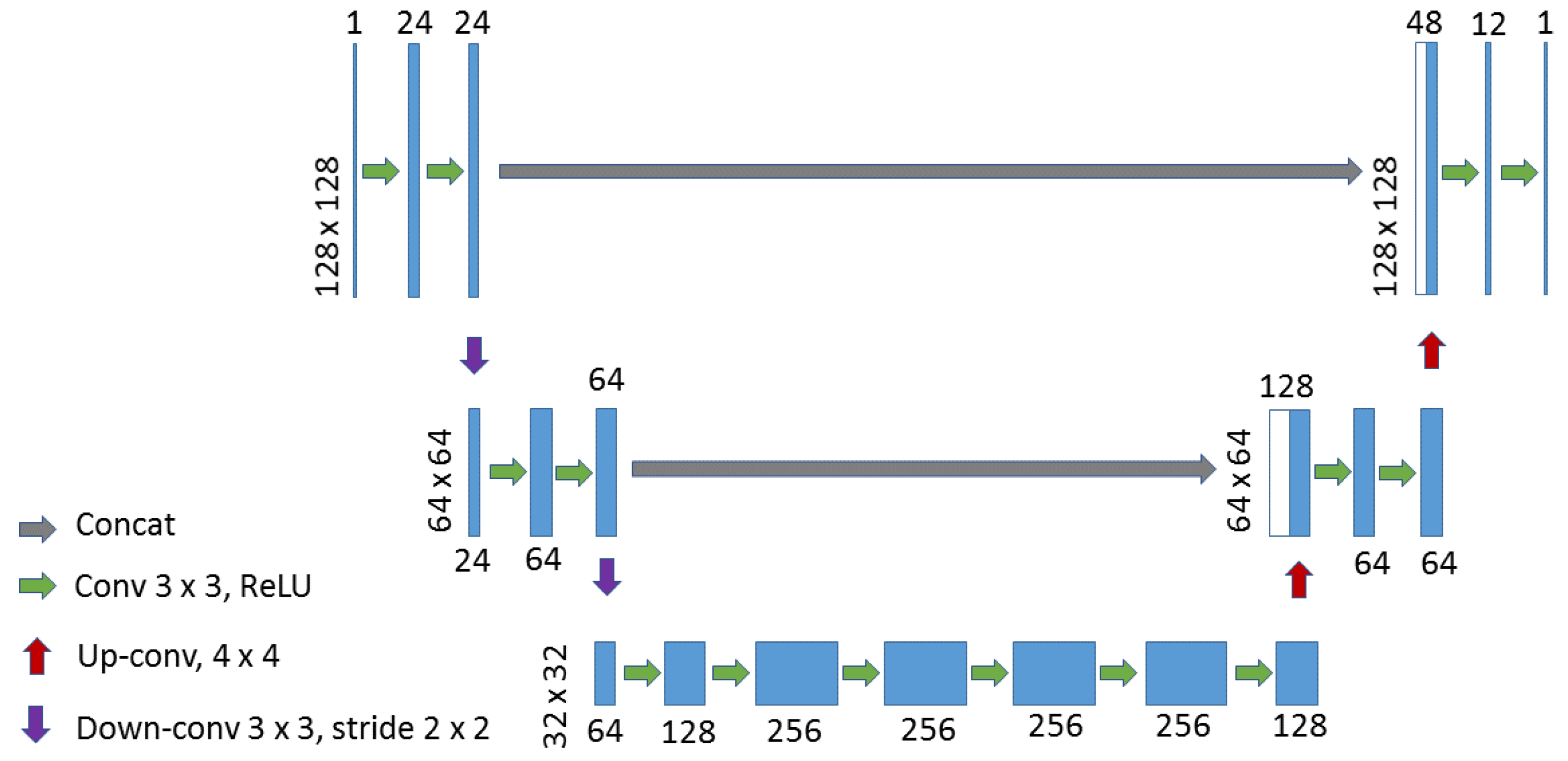
34]. The U-net network is symmetric and consists of three parts (shown in
Figure 1), down-sampling (left side), bottleneck (middle) and up-sampling (right side) paths. While up-sampling, each up-sampled layer is concatenated with the layer with the same size on the down-sampling path. This step is known as skip connection. Skip connections intend to provide local information while up-sampling. The models are able to generate less blurring results [
35].
This is also the basic network architecture used in our previous work [
29]. In that work, two modifications have been made compared with the original U-net [
31]. Zero-padding was applied at each convolution layer to achieve the same output size as the input image. Down-sampling was conducted using a convolutional layer with stride 2 instead of using max-pooling [
36]. The architecture of the network is shown in
Figure 1. In that study, the network architecture has shown that it can generate promising results for the building generalization task. In this paper, we intend to improve it by exploring two other architectures. In order to illustrate the improvements, this architecture is used as a baseline.
3.2. Residual U-net
Since building generalization mostly affects the boundary of the buildings, the pixel-wise difference between the input and output images are very small. In order to improve the generalization results, models with higher capacity need to be built. One of the solutions is to build deeper models, however, previous research already proved that simply increasing the number of convolutional layers does not improve the performance of CNNs [
37]. Degradation problems may occur. Therefore, the full pre-activation residual unit proposed for residual neural network [
37] was used to overcome such problems.
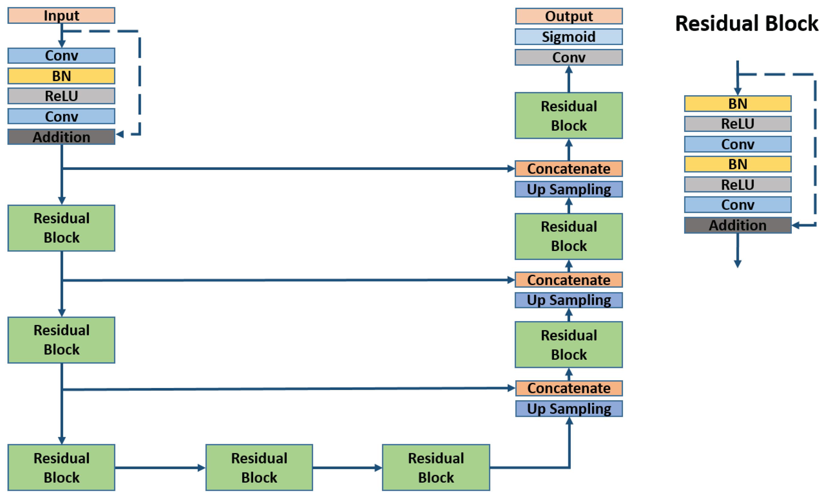
Following this idea, we replaced the convolutional layers in U-net by the residual unit, which consists of batch normalization (BN), ReLU (Rectified Linear Unit) activation and one convolutional layer (as shown in
Figure 2). The input of the residual unit is skip connected with the layer after convolution layers with addition. In this way, only the residuals between input and output of the residual unit are learned. By combining the residual units to U-net, the capacity of the model increased and the performance of the model should be improved. A similar idea has been successfully applied for road extraction from aerial images with binary labels [
32]. Such architectures show better performance compared with using a simple U-net architecture.
3.3. Generative Adversarial Network (GAN)
The results from our previous study [
29] show that the parallelism and rectangularity of the building patterns in some cases can not be preserved adequately. Another neural network architecture, which has great potential to tackle this problem, is the GAN [
33].
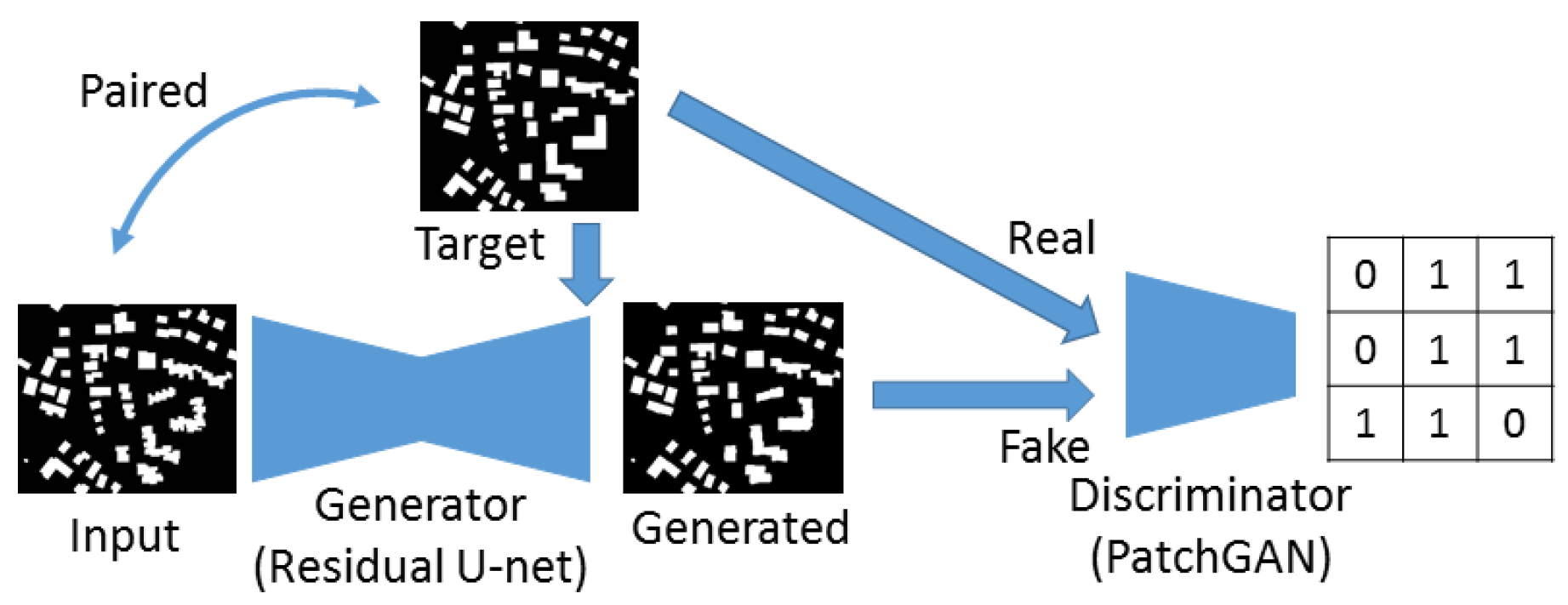
This kind of architecture iteratively trains two neural networks, a generator network and a discriminator network. The generator
G is used to capture the data distribution and generates samples similar to those drawn from training data. The discriminator
D estimates the probability that a sample comes from the real data, rather than being the outputs of generator. The discriminator provides an adversarial loss, which could force the generated images towards the target manifold [
38]. Such kinds of network architectures are currently often used for style transfer [
38,
39,
40], image super-resolution [
41], image inpainting, etc. The aim is often to generate photos as realistic as possible. However, for building generalization, we are not only aiming at generating simplified raster building maps at different scales, but the outputs should also look like the buildings in the maps. In this case, the term realistic for GANs means to achieve better rectangularity and parallelism of the building shapes.
Since large amounts of paired input and target images are available for this task, a supervised adversarial training [
42] was applied. It is similar to the image-to-image translation problem [
35], the supervised loss from the generator was combined with an adversarial loss from discriminator to optimize the model performance. The generator learns a mapping from input image
x to output image
y. This supervised loss
can be any standard loss, such as L1, L2 or cross-entropy, which measures the difference between the model output
and target output
.
At the same time, the discriminator learns a model which can compute the probability
that an input
y comes from the real data, rather than being the output of a generator with the following objective function
The final objective function to be optimized is
where
is a hyper-parameter which generates a weighted combination of the generator loss and adversarial loss. When
is too high, it performs similar to only using the generator. On the contrary, the model generates realistic outputs without correlation to the inputs.
In this work, the residual U-net is used as generator. Many generative networks, such as CartoonGAN [
38], CycleGAN [
39], also involve residual units to improve their performance. Therefore, we still consider that the residual blocks is a good choice for the generator. In general, there are two popular architecture for the discriminator. The early one, ImageGAN (as shown in
Figure 3), only predicts an overall score, whether the input of the discriminator is real or fake (e.g., GAN [
33], cGAN [
43], WGAN [
44]). Another very popular approach is PatchGAN [
35] (as shown in
Figure 4) which classifies small patches into real or fake (e.g., Pix2pix [
35], CycleGAN [
39], DiscoGAN [
45]). In our experiment, these two types of discriminators are compared. We trained the PatchGAN structure with a patch size 32 pixel to provide the adversarial loss.
5. Results and Discussion
In this section, results from the previously described three neural network architectures for building generalization are presented in the following five case studies. An 1.2 km × 1.2 km area outside our training data set was selected and then evaluated quantitatively for the three architectures at the three target map scales. Additionally, two randomly selected small areas outside the training area were evaluated at a specific target map scale 1:15,000 to demonstrate its ability to simplify and aggregate. Qualitatively, specific buildings with different orientations were generalized and a visual comparison was provided. The results at three target scale will be presented with best performed models from each neural network architecture. After that, we present the results where the best-performing residual U-net was applied on a large extent of data for a more detailed visual inspection. Finally, the observations will be summarized and discussed in the last subsection.
5.1. Quantitative Analyses on a Single Independent Test Area at Three Target Map Scales
An area to the south of our study area was selected, which does not have any overlap with our training data. Raster images of 2400 pixel × 2400 pixel at all three target scales were generated from rasterized CHANGE outputs. They are used as the target images for a quantitative evaluation of the models. The models were mainly evaluated based on the error rate, because we want to focus on the pixels where wrong predictions were made.
where
TP = true positive, which indicates the amount of building pixels correctly predicted as building;
FP = false positive, which indicates the amount of non-building pixels wrongly predicted as building;
TN = true negative, which indicates the amount of non-building pixels correctly predicted as non-building;
FN = false negative, which indicates the amount of building pixels wrongly predicted as non-building. Since the difference between the input and target image is small, the error rate of a direct use input compared with target is also listed (
Table 1). In further,
Table 2 provides the precision, recall and f1-score for the positive class.
From the results above, it is obvious that all the three methods were able to generate generalized outputs which were closer to the target output rather than the rasterized original building vectors. However, the residual U-net outperformed the other two approaches at all target scales. Even though GAN can not produce the best results, however, it is still better than the baseline approach U-net.
5.2. Experiments with the Specific Map Scale 1:15,000
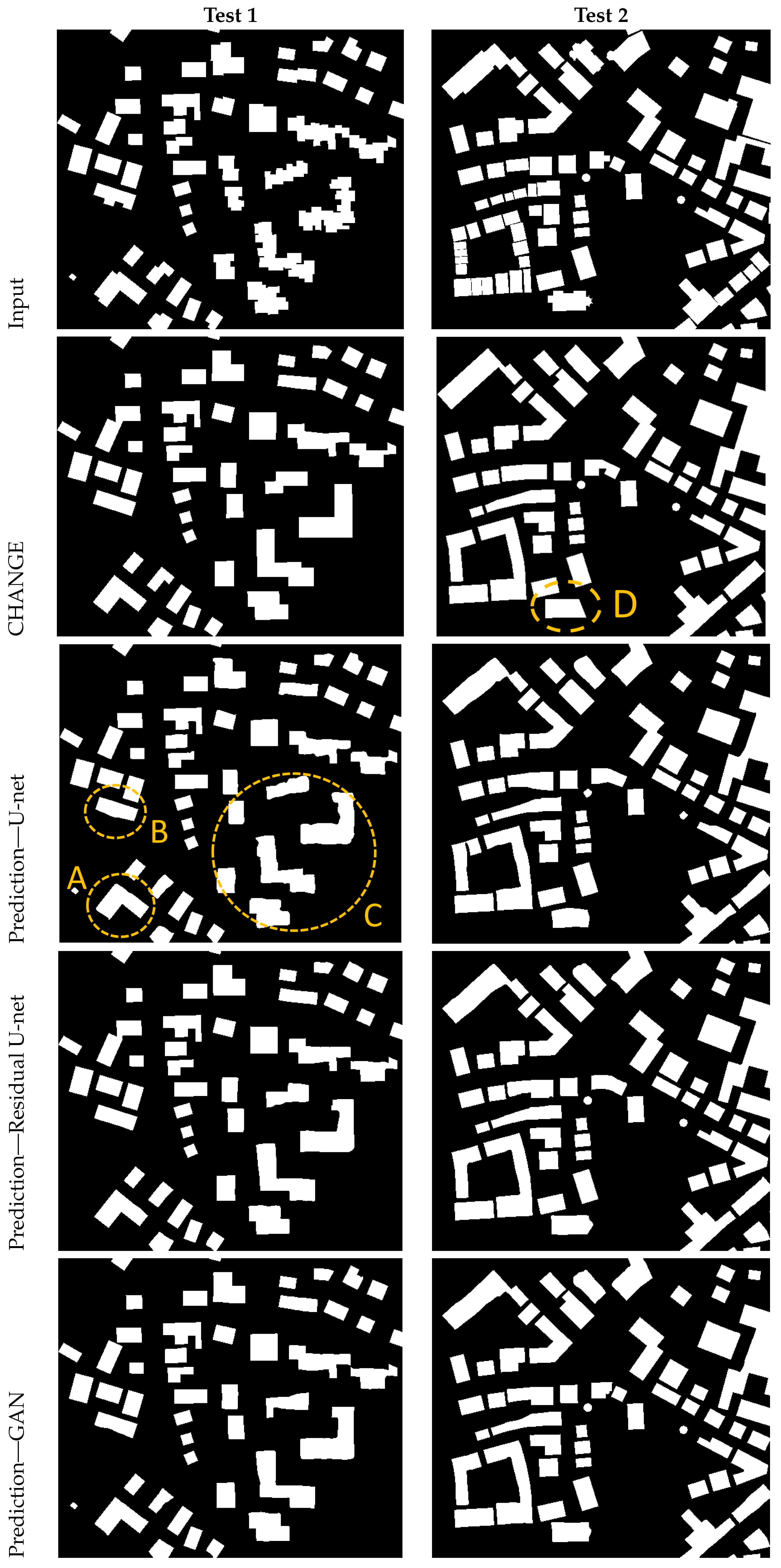
The following two tests have been conducted for building maps at target scale 1:15,000 (see
Figure 10). Test 1 investigates the simplification of certain building structures. The three encircled areas in
Figure 10 visualize the generalization capabilities of the U-net model:
A shows that the intrusions at the corners are filled;
B shows that the F-shaped building is simplified to a rectangle-similar to the target output produced by CHANGE. The area encircled in
C visualized that the system was capable of simplifying very complex building outlines: the many extrusions and intrusions were replaced by a smooth outline. Still, the outlines of U-net were not exactly straight lines, nor were the corners exact right angles, as given in the target output.
Then, we compared these three encircled areas with the corresponding parts of the predictions from residual U-net and GAN: the outlines were much closer to straight lines and the corners of the buildings were better preserved. The improvement by introducing residual blocks to the U-nets was obvious.
Still, there were some very small extrusions and intrusions. Note, however, that these visualizations were enlarged substantially in order to show the generalization effect appropriately. To illustrate the real size,
Figure 11 shows input image, target image and the predictions from three neural networks in the the dedicated target scale 1:15,000. It can be stated that the effect of generalization of our prediction was clearly positive: as opposed to the original image (left) scaled down to 1:15,000, the forms were simpler, no tiny details disturb the visual impression.
Test 2 in
Figure 10 investigated the aggregation where neighbouring objects can be merged. The input and target images were presented together with the predictions from three models. Clearly, the buildings close to each other were merged (see, e.g., the squared block in the lower left corner). The church in
D was generalized to a better representation compared with the target output from CHANGE. Compared with the prediction from U-net, the results from residual U-net achieved better straightness of the building borders and preserved some of the corners clearly.
In addition to the visual inspection, quantitative tests have also been conducted. For the two independent test sets mentioned above, we evaluated the target output with input image and the predictions from the models based on the error rate (
Table 3) and the corresponding precision, recall and f1-score on the positive class (
Table 4). The results show that the models did generate predictions much similar to the target output. The residual U-net outperformed the other two models, which was similar to the observation in the previous case study.
5.3. Experiments with Specific Buildings and Orientations
In order to evaluate the behaviour of the network with respect to typical building shapes, a test series of buildings has been produced. All the buildings have offsets and extrusions of different extents. In this test, also the potential dependency on the orientation was investigated by rotating the shapes in four different directions. The results are shown in
Figure 12 and
Figure 13. Please note that the size of the buildings is different—the longest dimension of buildings is 80m in
Figure 12 and 25 m in
Figure 13. The figures visualize the original image on the top and the generalization results in below.
It can be observed that the extrusions and intrusions are continuously eliminated with increasing scale. It is also clear, that the modifications of the building outlines are very subtle for the larger scales, and get more and more visible for the smaller scales. In
Figure 12 the offsets vanish with smaller scales, so does the annex in
Figure 13. The purpose of this experiment was mainly to check, if there is a dependency on the orientation of the buildings. This is not the case—obviously, the network has learned enough examples of extrusions, intrusions and offsets in different orientations, and is able to generalize them appropriately. A general observation can be made: compared with U-net and GAN, the residual U-net can generate buildings with much better preserved straight lines and corners.
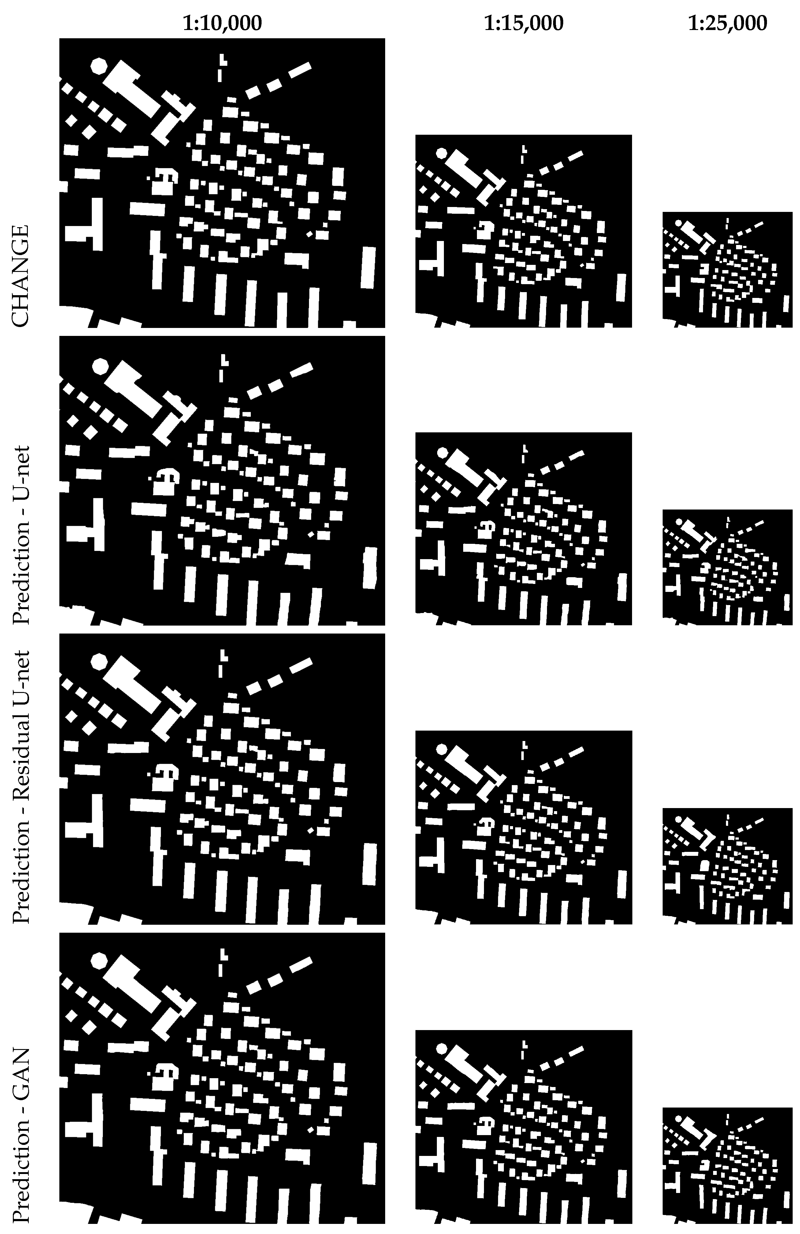
5.4. Map Series in Different Scales
The following visualizations show the same spatial extent at three different target scales (
Figure 14). In the top row, the solutions using CHANGE are given, whereas in the following rows the predictions with the three deep neural networks are given. For a detailed comparison, the same spatial extents at all three scales are visualized with images in the same size.
Figure 15 shows the generalization results at the three target map scales in their respective size.
From the results presented above, it is apparent that the models were able to both simplify existing outlines, eliminate too small buildings, and also merge adjacent buildings; i.e., the models contained a combination of different individual operators. The models involving residual blocks showed significantly better results compared with U-net. As for the generalization results at original target size scale (
Figure 15), the building outlines were simpler, no tiny extrusions and intrusions disturbed the visual impression.
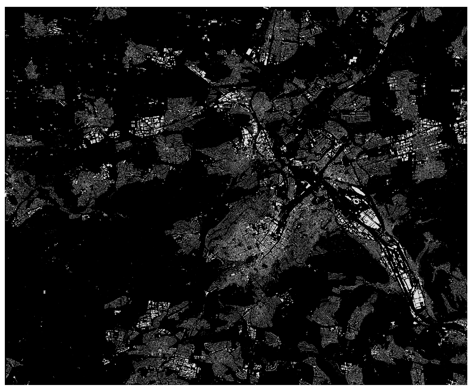
5.5. Results with a Large Extent of the Data Set
Figure 16 shows the result of a larger area in the target scales 1:10,000, 1:15,000 and 1:25,000, where the same spatial extents are visualized with images in the same size. The extent comprised both residential buildings and industrial buildings, as well as an inner city area. It can be seen that the residual U-net was able to produce appropriate simplifications for the different building types, i.e., rectangular shaped residential buildings and irregular shaped buildings in the city center, where different individual buildings were merged. It was also visible that small buildings have been eliminated in the smaller scales.
5.6. Discussion
In the case studies shown above the predictions of the neural networks are evaluated both quantitatively and qualitatively. A visual inspection of the results clearly indicated that the networks have learned the simplification of the buildings for the respective scales: small buildings are eliminated in smaller scales; close, neighboring buildings are aggregated, and outlines are simplified by eliminating small extrusions and indentations. This can nicely be observed in
Figure 10 test 1, where the buildings with the complicated ground plans in the right part of the image have been simplified to L-shaped outlines.
Our baseline solution U-net can already provide valid simplification for buildings. After combination with the residual units, a significant improvement has been achieved both in the quantitative test and visual inspection. By further introducing a GAN-like discriminator, unfortunately, the network did not improve its performance in the quantitative evaluation. As observed and stated in the work of image-to-image translation [
35], GANs are effective at generating outputs of highly detailed or photographic objects and scenes, however, they cannot achieve a better performance than simply using L1 regression for the semantic segmentation task. Since a similar network architecture for semantic segmentation was used in this work, the previous observation can also be confirmed that simply introducing GAN-like discriminators does not necessarily improve the prediction results in a quantitative evaluation.
Qualitatively, the residual U-net and GAN achieved relatively similar results based on our visual inspection. However, visual inspection is subjective, only a systematic assessment by human map readers can provide a valid comparison. Furthermore, training the GANs is more computational expensive than training a residual U-net. Therefore, we conclude that introducing GAN-like discriminators, such as ImageGAN or PatchGAN, do not significantly contribute to the model performance.
Even though the residual U-net can produce predictions with much clearer outlines, it is still sometimes not as perfect as the classic solutions in vector space. The characteristic features of some of the individual buildings, namely rectangularity and parallelism are not always well preserved or enhanced. In many cases, the models do not generate exact straight lines. These small defects could be cleaned up in a post-processing step, using e.g., an approach proposed by Sester and Neidhart [
50], which explicitly takes these constraints into account and optimizes it in an adjustment process.
The visualizations showing the original sizes of the target scales (e.g.,
Figure 11 and
Figure 15) reveal that the results of the predictions can be used for presentation graphics: the generalization—i.e., simplification of the outline, reducing the content, as well as preserving the overall structure of the buildings and building structure—is clearly achieved with the approach.
6. Conclusions
In summary, this work was intended to be a proof-of-concept whether applying or slightly modifying existing DCNNs could achieve satisfying generalization results. The results indicate that this was successful. In this paper, three neural network architectures, namely U-net, residual U-net and GAN, have been evaluated on the cartographic building generalization task. The results show that all these networks could learn the generalization operations in one single model in an implicit way. The residual U-net, which combines the benefits of U-net’s skip connection and ResNet’s residual unit [
51], outperforms the other two types of models. GAN was applied and tested with two types of discriminators and multiple weighting factors. Unfortunately, it could not significantly enforce the generator to produce generalized building patterns with better parallelism and rectangularity as we had hoped. Therefore, the residual U-net is considered as a proper solution for this task.
However, there are several avenues to go in the near future: obviously, the simple L2 loss does not strongly enforce that characteristic building shapes are preserved (such as parallelism, rectangularity). Future work will be devoted to investigating other loss functions or adaptations on current loss function, which could be applied to enforce such constraints. Also, other generalization functions will be tested, such as typification or displacement.
This work focused on learning the cartographic generalization operations in raster space, which needs a conversion between vector and raster. At the moment, we are investigating the ability to generate building maps at different map scales from high resolution areal images, where image segmentation models directly generate outputs in raster. These raster maps are then fed into the learned models to produce building maps in different scales. On the other hand, we will also explore the use of deep learning in vector space by creating a representation of the building outline, which can be represented or simplified using approaches such as long short-term memory (LSTM) [
52], or a graph convolutional neural network [
53]. A possible representation could be a vocabulary, which was proposed for a streaming generalization approach [
54].


