A Multilevel Terrain Rendering Method Based on Dynamic Stitching Strips

Abstract

High-quality terrain rendering has been the focus of many visualization applications over recent decades. Many terrain rendering methods use the strategy of Level of Detail (LOD) to create adaptive terrain models, but the transition between different levels is usually not handled well, which may cause popping artefacts that seriously affect the reality of the terrain model. In recent years, many researchers have tried using modern Graphics Processing Unit (GPU) to complete heavy rendering tasks. By leveraging the great power of GPU, high quality terrain models with rich details can be rendered in real time, although the problem of popping artefacts still persists. In this study, we propose a real-time terrain rendering method with GPU tessellation that can effectively reduce the popping artefacts. Coupled with a view-dependent updating scheme, a multilevel terrain representation based on the flexible Dynamic Stitching Strip (DSS) is developed. During rendering, the main part of the terrain model is tessellated into appropriate levels using GPU tessellation. DSSs, generated in parallel, can seamlessly make the terrain transitions between different levels much smoother. Experiments demonstrate that the proposed method can meet the requirements of real-time rendering and achieve a better visual quality compared with other methods.

1. Introduction

Terrain visualization plays an important role in many applications, such as Geographic Information System (GIS), computer games, and virtual reality. For example, the real-time visualization of terrain in many virtual globe applications provides an efficient and fantastic way of visiting landscapes in the world on a personal computer. Therefore, the rendering effect is a crucial element that has a great influence on the reality of the terrain models [1]. In recent decades, with the increasing size of terrain models and higher visualization quality requirements, terrain rendering methods have been facing new challenges.

Level of Detail (LOD) is a popular technique used in terrain rendering. It can reduce unnecessary details of the terrain models and assign appropriate resolutions for areas that have different roughness or distances to the viewpoint [2]. However, the problem of inconsistency between different levels arises when using LOD, which may result in obvious visual artefacts that seriously affect the reality of the terrain model, such as popping artefacts [3,4]. The popping artefacts will bring sudden changes of the terrain model which make the user lost in the scene when wandering. In terms of height map-based terrain rendering methods, the popping artefacts could be reflected by the height difference change of coarse models at different levels. As shown in Figure 1, by performing ray casting along the height direction, the height difference between the coarse model and the original model along each ray can be calculated and we can utilize it to evaluate the popping artefacts quantitatively.

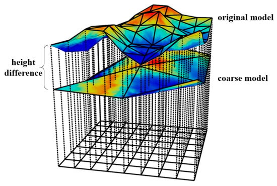
Figure 1. Evaluating popping artefacts using height difference.

Traditional methods solve this problem by using operations such as complex geomorphing [5] or texture blending [6] to obtain a smooth transition. However, with the great improvement of graphics hardware, these methods are not suitable for modern Graphics Processing Unit (GPU) due to the large CPU-GPU data transmission [7]. Lee et al. [8] proposed a GPU-based vertex relocation method by introducing the concept of attraction and elastic forces to preserve terrain features, which can reduce the popping artefacts in rugged regions and is faster than CPU-based methods. In the last few years, some terrain rendering methods have begun to utilize the advantages of GPU tessellation, which can tessellate the original terrain patches view-dependently into finer meshes with appropriate details in real time. However, in order to guarantee seamless rendering, these methods limit the terrain patches in several discrete and fixed tessellation levels [9,10]. Nevertheless, visual popping artefacts persist.

To achieve smooth terrain changes when using GPU tessellation, a real-time terrain rendering method is proposed in this study. A quadtree-based multilevel model is designed to represent the terrain, and correspondingly, a view-dependent terrain LOD scheme is designed to update the model in real time. The primary parts of the terrain model, separated into blocks and organized by a quadtree, are entirely generated in the GPU tessellation stage. A dynamic strip structure created at run time under a multithread strategy is introduced to fill the gaps between terrain blocks at different levels. The main contribution of our method is that we propose the dynamic strip structure to achieve smooth transitions between different levels as viewpoint moving. By introducing this structure, the terrain can be adjusted in a continuous manner rather than being limited to several fixed tessellation levels. Thus, obvious popping artefacts can be avoided. Several comparison experiments are conducted to demonstrate the visual effect and efficiency of our method.

2. Related Work

There are various representations of terrain, such as voxels, procedural terrain, and height maps [6]. Considered as the 3D version of pixels, voxels are able to represent volumetric terrain features, such as caves and overhangs [11,12,13]. However, to represent a large and detailed terrain model, billions of voxels may be needed, which will cause intensive memory requirement and are inappropriate for real time rendering [14].

Widely used in gaming, procedural terrain is not generated on the basis of the natural world [15]. Instead, in many cases, the terrain surface is completely described by a density function and is procedurally created at run time [16]. In this way, vast or infinite terrains with high quality can be generated without human intervention [17]. But at the same time, the creation process is usually random and is difficult to control [18]. Thus, procedural terrain is not suitable for the visualization of real terrain.

Height maps, the most popular terrain representation [14], can be acquired through various means, such as aerial photogrammetry and remote sensing satellites [19]. Considering the difference of the base structure, terrain rendering methods using height maps can be classified into Triangulated Irregular Network (TIN) based methods, regular or semi-regular structure-based methods, and methods combining TIN and semi-regular structure. Recently, some new GPU properties have been introduced into these methods for improved visual quality or performance.

2.1. Triangulated Irregular Network

By sampling the height map non-uniformly, TIN can distribute more triangles to areas with more details. Compared with regular grids, the generation of TIN usually needs a more complex triangulation process such as Delaunay triangulation [20], and it is more difficult to create a multiresolution mesh based on TIN. Schroeder et al. [21] used the decimation method to construct multiresolution TIN model. While some other methods triangulate the terrain surface recursively and encode the history of refining and coarsening operations in the pre-processing stage to create a multiresolution model [22,23]. Moreover, some studies utilized the iterative edge collapse and vertex split method [24,25], which usually need complicated structures to store the vertex topological relationships [26]. Above multiresolution triangulation methods offer the possibility of a continuous range of terrain resolutions [27], but a sudden change can be observed in the transition. Hoppe [28] introduced previous work about View-Dependent Progressive Mesh (VDPM) [29] into terrain rendering. With the help of edge collapsing and vertex splitting, a smooth transition between different levels was realized. Bertilsson and Goswami [30] divided the terrain into patches at the same level with the same dimensions, then individually triangulated each patch, which was very suitable for parallel processing.

2.2. Regular or Semi-Regular Structure

The simple structure of a regular grid brings substantial convenience to terrain data storage and management, and facilitates getting the index of a vertex using its coordinates. However, its regular subdivision requires a greater number of triangles to obtain the same accuracy as TIN [31]. An example for a regular grid is the combination of the texture mipmap with height map [32]. Moreover, inspired by texture clipmap, Losasso and Hoppe [6] proposed the geometry clipmap. They represented the terrain by several nested regular rectangle grids centered on the viewpoint, which form a multiresolution structure by themselves. Later, a GPU implementation of the geometry clipmap was presented by Asirvatham and Hoppe [33]. Based on the geometry cilpmap, interactive editing of terrain can also be achieved through sketch-based input [34]. Besides, projective grid mapping is another regular grid based method which provides a new way to render terrain efficiently [35,36]. Its basic idea is projecting a regular grid in the screen space onto the terrain plane. To utilize the benefits of ray-tracing and mesh-rendering, Livny et al. [37] sampled the terrain by fast ray shooting, and they didn’t constrain the persistent sample grid, which was able to generate meshes with different subdivision manners.

Semi-regular structure is a series of right triangles organized by a quadtree or binary tree and is usually called Right-Triangulated Irregular Networks (RTIN) [38]. Based on RTIN, it is easy to build an adaptive triangle mesh according to some view-dependent error metrics. The refining and coarsening of terrain mesh is realized by longest edge bisection (triangle splitting) and vertex removal (triangle merging), respectively. Besides, the structure of RTIN provides plenty of convenience for designing an efficient neighbor finding scheme [39,40]. To guarantee a seamless terrain mesh, a restricted quadtree structure [41] and constraints for triangle splitting and merging [42] are required. By recursively removing vertices and polygons inside the quadtree node in a top-down manner, Lindstrom et al. [43] proposed a terrain rendering method that achieves continuous LOD in the polygon level. However, as the viewpoint moving, a phenomenon called vertex popping may occur. To eliminate this artefact, an efficient geomorphing operation was introduced by Röttger et al. [44]. Similar to other methods based on semi-regular structure, Lindstrom et al., operate the terrain model at the vertex level and try to make each triangle count, which limits the possibility of rendering massive terrain data on the GPU. In the study of Levenberg [45], clusters of geometry called aggregate triangles are taken as the basic operation object, which can be cached on the video memory, thus heavy LOD computation on CPU was lightened.

2.3. Combination of Semi-Regular Structure and TIN

Some methods make use of the advantages of both semi-regular structure and TIN, such as QuadTIN [46,47] and 4–8 meshes [48]. These methods divide the terrain into a quadtree or binary tree of blocks, where each block is a TIN patch generated in the pre-processing stage. These TIN patches are sent to the GPU as a whole without complex updating operations at run time, which greatly reduces the CPU computing load and makes it possible to render massive terrain data in real time [49]. Compared with methods based on semi-regular structure, both the visual effect and performance are improved when using combination methods [50].

Moreover, there is another way to use both the advantages of grid and TIN, which combines the two structures together to create a hybrid terrain model [51,52]. It has the advantage of using finer resolution TINs to represent complex terrain regions or man-made constructions. To avoid artefacts such as visual discontinuities and overlapping triangles at the boundary, the join part of grid and TIN should be locally remeshed [53]. For this purpose, a Hybrid Meshing (HM) algorithm [54,55] was proposed which connects different terrain representation through a local, cell-based strategy without modifying the original terrain data. Paredes et al. [56] extended the work of HM algorithm to support rendering of multiresolution TIN and grid models. Later, Paredes et al. [57] improved their work on memory storage and parallelism.

2.4. GPU Tessellation

Hardware tessellation was added into the GPU rendering pipeline since OpenGL 4.0 and Direct3D 11. During the tessellation stage, a coarse input patch can be subdivided into many smaller primitives on the fly, which is very efficient and can save much memory [58]. This property is very suitable for displacement mapping with height maps [59], and an increasing number of researchers are focusing on how to apply GPU tessellation to terrain rendering. Fernandes and Oliveira [60] broke the planar input mesh into subpatches with equal size to obtain a terrain model with variable densities. However, their uniform division pattern limits the adaptive refinement of the terrain. Cantlay [61] implemented a crack-free terrain surface with DirectX 11 tessellation by adjusting the tessellation factors, but this implementation did not consider the roughness of local terrain areas, which could cause many unnecessary triangles. Rather than changing the tessellation factors, Yusov and Shevtsov [62] used vertical skirts [63] to hide gaps, but this could cause the transition part between terrain patches to become unnatural. Song, Yang, and Ji [10] applied the GPU tessellation to the geometry clipmaps and a higher efficiency was acquired compared with the CPU-based geometry clipmaps algorithm. Some studies utilized the hierarchical structure of quadtree to create a coarse LOD, after which the patches of the quadtree nodes were tessellated into different levels [64,65]. Instead of quad patches, Mikhaylyuk et al. [66] used triangle patches at several levels of details to subdivide a sphere model of the Earth, which can create a more adaptive mesh. However, to avoid the cracks between terrain patches, the tessellation levels are restricted to several fixed values, which can cause visual popping artefacts [9], as shown in Figure 2.

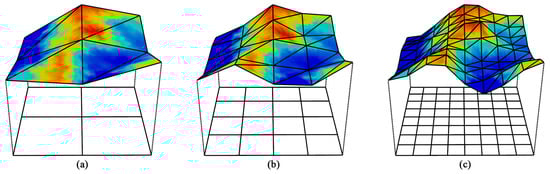
Figure 2. Illustration of popping artefacts caused by using several limited levels at power of 2: (a) Tessellation level = 2.0. (b) Tessellation level = 4.0. (c) Tessellation level = 8.0.

We propose a new terrain rendering method based on the GPU tessellation. With the help of a dynamic strip structure, the gaps between adjacent terrain patches are removed and the levels of terrain patches can be adjusted in a continuous way; therefore, smooth transitions are realized between different LODs, which achieves a better visual effect.

3. Methods

An overview of our method is shown in Figure 3. In the preprocessing stage, terrain data and object-space error are loaded into the memory. We compute the object-space error based on height difference between coarse models and the original model and convert it into screen-space error in the CPU stage (see Section 3.3.1). The hierarchy of the multilevel terrain model is constructed by a quadtree. Each quadtree node represents a terrain block (called M-block). Once a quadtree node splits, besides four children nodes, there is also a small square (called P-block) placed in the center. Moreover, a stitching strip structure (called DSS) between terrain blocks is also introduced. Under a view-dependent updating scheme, terrain block meshes are generated with appropriate levels in the GPU. At the same time, stitching strips are constructed dynamically in parallel to fill the gaps between the terrain blocks. Finally, a multilevel terrain model that changes smoothly between different levels is obtained. The specific implementation is as follows.

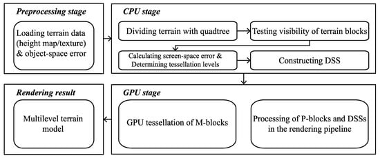
Figure 3. Flowchart of the proposed terrain rendering method.

3.1. Multilevel Model with Dynamic Stitching Strip

In the proposed model, the terrain is divided into three different types of areas based on a quadtree (Figure 4): (1) main blocks (M-blocks); (2) patching blocks (P-blocks); and (3) Dynamic Stitching Strips (DSSs). As the key element of the whole terrain model, the DSS also plays an important role in enabling the smooth change of M-blocks, and thus reduces the popping artefacts and guarantees a seamless rendering.

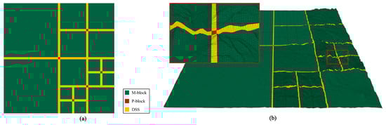
Figure 4. Three types of areas in the terrain model: (a) A 2D projection of the model. (b) The 3D model with wireframe overlay which has the same division with (a).

3.1.1. M-Block

M-blocks are the main body of the terrain model. Each M-block corresponds with a leaf node in the quadtree. For each quadtree node, we need a structure to store all the information dealing with the generation of an M-block. We call this structure M-block data (MBD), which has the following items:

$$\mathrm{MBD}=\left\{\mathrm{Id},\mathrm{Position},\mathrm{Size},{\mathrm{F}}_{\mathrm{tessellation}},{\mathrm{L}}_{\mathrm{quadtree}},{\mathrm{Pts}}_{\mathrm{child}},{\mathrm{Ids}}_{\mathrm{neighbour}}\right\}$$

The $\mathrm{Id}$ field is used for indexing the M-blocks. With an M-block, the $\mathrm{Id}$ of which is $k$, the $\mathrm{Ids}$ of its children can be expressed as $4\left(k+1\right)$, $4\left(k+1\right)+1$, $4\left(k+1\right)+2$, $4\left(k+1\right)+3,$ respectively, starting from the lower left corner anti-clockwise (Figure 5). The $\mathrm{Id}$ field is not only used for indexing M-blocks, but also helpful in creating DSS (see Section 3.1.3). The $\mathrm{Position}$ and $\mathrm{Size}$ fields encode the 2D coordinates and the side length of an M-block respectively. ${\mathrm{F}}_{\mathrm{tessellation}}$ is the tessellation factor that determines the LOD of an M-block when tessellating it into a finer mesh in the GPU tessellation stage. According to the above three fields, we can locate an M-block and obtain the geometry of it. ${\mathrm{L}}_{\mathrm{quadtree}}$ indicates the hierarchy of the node in the quadtree. ${\mathrm{Pts}}_{\mathrm{child}}$ includes four pointers of child nodes. ${\mathrm{Ids}}_{\mathrm{neighbour}}$ is an array with four elements encoding the indices of adjacent DSSs and is used for creating DSS (see Section 3.2). Besides, the four edges of an M-block are represented by $a~d$ (Figure 5b).

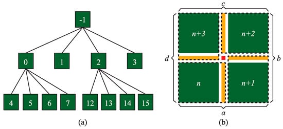
Figure 5. Indexing scheme based on quadtree: (a) Indices of quadtree nodes. (b) The Dynamic Stitching Strip (DSS) and M-block in the same dotted rectangle are bound together; $a~d$ represent the four edges of an M-block.

3.1.2. P-Block

P-blocks are used to fill the holes caused by quadtree division (Figure 5b). Based on the $\mathrm{Position}$ and $\mathrm{Size}$ in MBD, it is easy to acquire the geometry of a P-block after splitting an M-block.

3.1.3. DSS

After an M-block splits, four children are created with gaps between them. To obtain a seamless terrain mesh, four DSSs are created to fill the gaps caused by M-block splitting. The DSS works in a stitching manner; thus, we should know which M-blocks are going to be stitched. For this purpose, we can bind each M-block (except the root node) with its anti-clockwise adjacent DSS (Figure 5b). For the sake of illustrating the relationship between M-blocks and DSSs, we added some intervals between them. However, there are no such intervals in the actual structure. Thus, each DSS can share the same index with its corresponding M-block. These indices are stored in the ${\mathrm{Ids}}_{\mathrm{neighbour}}$ as noted above.

3.2. Construction of DSS

3.2.1. Encoding Adjacency Relationship

After the division of the terrain, M-blocks at different quadtree levels are separated by gaps (Figure 6a). To fill these gaps with DSSs, the vertices on the common edge of DSSs and M-blocks must coincide with each other (Figure 6b) and then be triangulated into a seamless mesh of strips (Figure 6c). From Figure 6, although we can directly point out the M-blocks that are adjacent to the DSSs, it is still necessary to record the adjacency relationship of DSSs to obtain all the vertices of a DSS.

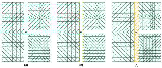
Figure 6. Creation process of a DSS: (a) M-blocks separated by gaps. (b) Original vertices needed to generate the DSS. (c) Triangulated DSS.

Before creating a DSS, only the MBDs of M-blocks exist. We use the ${\mathrm{Ids}}_{\mathrm{neighbour}}$ field to assist the creation process. For the four edges $a~d$ (Figure 5b) of an M-block, their adjacent DSS indices are stored in ${\mathrm{Ids}}_{\mathrm{neighbour}}$[0]~${\mathrm{Ids}}_{\mathrm{neighbour}}$[3], respectively. The values of the indices are obtained in the node splitting process. Let us suppose a node with an index $n$, and that the values of its ${\mathrm{Ids}}_{\mathrm{neighbour}}$ are $DssId\_a$, $DssId\_b$, $DssId\_c$, and $DssId\_d$. Then, we can calculate the values of ${\mathrm{Ids}}_{\mathrm{neighbour}}$ for its children nodes according to Table 1.

Table 1. Calculate values of ${\mathrm{Ids}}_{\mathrm{neighbour}}$ for children nodes.

Children Nodes Positions	$\mathbf{I}\mathbf{d}{\mathbf{s}}_{\mathbf{n}\mathbf{e}\mathbf{i}\mathbf{g}\mathbf{h}\mathbf{b}\mathbf{o}\mathbf{u}\mathbf{r}}\left[0\right]$	$\mathbf{I}\mathbf{d}{\mathbf{s}}_{\mathbf{n}\mathbf{e}\mathbf{i}\mathbf{g}\mathbf{h}\mathbf{b}\mathbf{o}\mathbf{u}\mathbf{r}}\left[1\right]$	$\mathbf{I}\mathbf{d}{\mathbf{s}}_{\mathbf{n}\mathbf{e}\mathbf{i}\mathbf{g}\mathbf{h}\mathbf{b}\mathbf{o}\mathbf{u}\mathbf{r}}\left[2\right]$	$\mathbf{I}\mathbf{d}{\mathbf{s}}_{\mathbf{n}\mathbf{e}\mathbf{i}\mathbf{g}\mathbf{h}\mathbf{b}\mathbf{o}\mathbf{u}\mathbf{r}}\left[3\right]$
lower left	$DssId\_a$	$4\left(n+1\right)$	$4\left(n+1\right)+3$	$DssId\_d$
lower right	$DssId\_a$	$DssId\_b$	$4\left(n+1\right)+1$	$4\left(n+1\right)$
upper right	$4\left(n+1\right)+1$	$DssId\_b$	$DssId\_c$	$4\left(n+1\right)+2$
upper left	$4\left(n+1\right)+3$	$4\left(n+1\right)+2$	$DssId\_c$	$DssId\_d$

Proceeding with the example presented in Figure 7, we can see that M-block $B1$ has two adjacent DSSs, $S1$ and $S0$, so its ${\mathrm{Ids}}_{\mathrm{neighbour}}$ is {null, null, 1, 0} (null indicates that the edge has no adjacent DSS). The adjacent DSSs of $B1’$s children node $B11$ are $S11$, $S10$, $S1$, and $S0$, so the ${\mathrm{Ids}}_{\mathrm{neighbour}}$ of $B11$ is {11, 10, 1, 0}. Similarly, we can observe that the ${\mathrm{Ids}}_{\mathrm{neighbour}}$ of $B11’$s children node $B49$ is {11, 10, 49, 48}. All the ${\mathrm{Ids}}_{\mathrm{neighbour}}$ of $B11$ and $B49$ are agreement with Table 1.

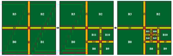
Figure 7. Determine values of ${\mathrm{Ids}}_{\mathrm{neighbour}}$ while an M-block splitting: (a) The adjacent DSSs of $B1$ are $S0$ and $S1$. (b) $B1$ splits into four child nodes. (c) $B11$ splits into four child nodes.

Once the relationship between DSSs and M-blocks is encoded, based on the index of a DSS, it becomes easy to find the adjacent M-blocks of a DSS by searching for the index of the DSS in the ${\mathrm{Ids}}_{\mathrm{neighbour}}$.

3.2.2. Generating Coincident Vertices

The vertices of a DSS are obtained by tessellating edges of adjacent M-blocks in CPU. To guarantee seamless rendering, the vertices on the common edges of DSSs and M-Blocks coincide with each other. So we use the same tessellation manner as the fractional even spacing scheme of GPU hardware tessellation [67]. Moreover, to ensure the high efficiency of the generation process, a multithread strategy is adopted, which will be discussed in Section 4.2.

3.2.3. Triangulating the Vertices of DSS

After the previous steps, all the needed vertices for creating a DSS are obtained. Because these vertices on the two sides of a DSS are not distributed uniformly or symmetrically, triangulating them sequentially (Figure 8b) is not a good option, as it will result in unnatural visual artefacts, such as thin triangles (Figure 8a). The main principle of our triangulation algorithm is shown in Figure 8c: because the vertices of a DSS are distributed on two parallel lines, the three vertices of a triangle cannot be on the same side. Vertex $v_0$ and $v_1$ are first connected as an edge, and then the vertex $v_3$ that is nearest the perpendicular bisector $l$ of $v_0{v}_1$ is selected to form a triangle. Following this principle, the vertices in Figure 8b are reconnected using our triangulation algorithm (Figure 8d). The pseudo code is shown in Algorithm 1.

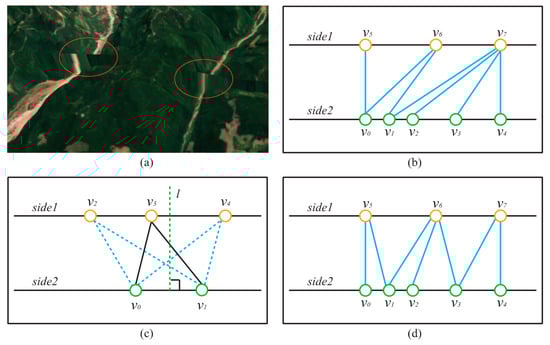
Figure 8. Triangulation of DSS: (a) Artefacts caused by thin triangles. (b) Connect the vertices sequentially. (c) The principle of our triangulation algorithm. (d) Connect the vertices based on our method.

It is noteworthy, that we adopt a parallel way to efficiently build DSSs. After encoding the adjacency relationship, several worker threads are created to generate the vertices. When the vertex generation task is completed, these threads are then used to execute the triangulation task.

Algorithm 1 Dynamic Stitching Strip Triangulation

1: Input: original vertices on both sides of a DSS

2: for each side do

3:     set $n$ as the number of vertices on the current side

4:     for $i$ = 0 to $n-2$ do

5:         select two adjacent vertices $a_i$, $a_{i+1}$ from the current side

6:         compute the perpendicular bisector $l$ of segment $a_i{a}_{i+1}$

7:         find the vertex $b_j$ which is nearest $l$ from the other side

8:         make triangle $\Delta a_i{a}_{i+1}{b}_j$

9:     end for

10: end for

3.3. View-Dependent Terrain Reconstruction

While the viewpoint moving, the terrain model is reconstructed accordingly, which involves two stages: firstly, the quadtree structure is updated in a top-down manner; and secondly, the ${\mathrm{F}}_{\mathrm{tessellation}}$ of each M-block is recalculated to meet the current error requirement. Moreover, a hierarchical view frustum culling strategy is applied to reduce the unnecessary terrain data in the reconstruction process.

3.3.1. Multilevel Updating Strategy

We first demonstrate the view-dependent error metric. The average vertical errors between the original finest model and M-blocks at different levels are used as the object-space error $\delta$. Next we need to convert $\delta$ into the screen-space error $\rho$. The ratio relationship between $\rho$ and $\delta$ in the view frustum (Figure 9) can be represented by the following equation:

$$\frac{y/2tan\left(\phi /2\right)}{d}=\frac{\rho }{\delta }$$

(1)

where $y$ is the vertical size of the viewport, $\phi$ is the field of view, $d$ is the distance from viewpoint to the M-block. As the program running, the viewport is seldom resized, meaning that $y$ and $\phi$ will not change, hence we can denote $y/2tan\left(\phi /2\right)$ as $\lambda$, which is a constant. So Equation (1) can be written as:

$$\rho =\lambda \frac{\delta }{d}$$

(2)

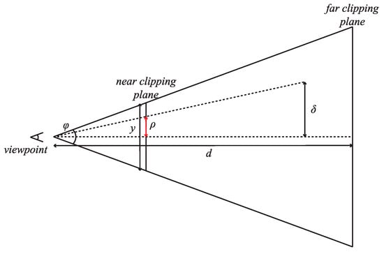
Figure 9. Computation of screen-space error $\rho$.

However, for height map-based terrain rendering methods, the vertical error that we actually observe is affected by the view direction. As shown in Figure 10a, $\delta$ is the original object-space error of an M-block. But when looking along the view direction $\overrightarrow{e}$, the object-space error actually observed is $\delta \prime =\delta sin\theta$, where $\theta$ is the angle between $\overrightarrow{e}$ and the normal vector $\overrightarrow{n}$ of the block plane (Here we take the unit vector along the positive Z axis as the normal, as the terrain plane before displacement is parallel with the XOY plane). Thus, the corresponding screen-space error $\rho$ can be calculated as shown in Equation (3):

$$\rho =\lambda \frac{\delta }{d}sin\theta$$

(3)

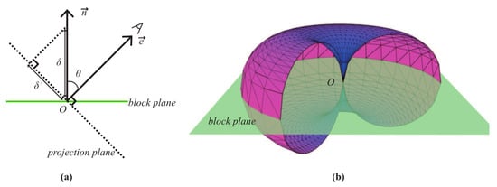
Figure 10. View-dependent error metric: (a) View direction affects the object-space error. (b) Geometric representation of the boundary condition of node splitting.

For each M-block, 32 object-space errors ${\delta }_i\left(i=1, 2,\dots , 31, 32\right)$ at different tessellation levels (${\mathrm{F}}_{\mathrm{tessellation}}=2, 4,\dots , 62, 64$) are computed in the pre-processing stage. Based on them, the corresponding screen-space error ${\rho }_i\left(i=1, 2,\dots , 31, 32\right)$ can be calculated following Equation (3).

While the tessellation level increasing, the mesh of the M-block becomes finer, and the value of ${\delta }_i$ and ${\rho }_i$ decreases. To decide whether an M-block (leaf node) needs to split or not, the minimum screen-space error ${\rho }_{32}$ is computed by setting $\delta$ = ${\delta }_{32}$ in Equation (3), then ${\rho }_{32}$ is compared with the screen-space error threshold ${\rho }_{thr}$. If ${\rho }_{32}>{\rho }_{thr}$, which indicates that the M-block is still not fine enough even at the finest level, the node will split into four children; otherwise, the node will remain and be adjusted in the next updating stage. A portion of the geometric representation [20] of the relationship between ${\rho }_{32}$ and ${\rho }_{thr}$ is shown as Figure 10b. It is a horn torus without a hole in the center. When the viewpoint is on the surface of the torus, the computed ${\rho }_{32}$ just equals to ${\rho }_{thr}$. In cases when the viewpoint is inside the torus, the computed ${\rho }_{32}$ is greater than ${\rho }_{thr}$, meaning that current fineness of the M-block cannot satisfy the requirement of ${\rho }_{thr}$. So in order to meet the requirement of ${\rho }_{thr}$, we need to make the mesh of the M-block finer to reduce ${\delta }_{32}$. However, ${\delta }_{32}$ is the smallest object-space error which cannot be reduced anymore, therefore, the only way to meet the requirement is splitting the node into four children to get finer meshes. It is noteworthy that although the update of quadtree structure can be achieved by merging and splitting the nodes, our method implements this by constructing a full quadtree in advance and selecting the needed nodes in the updating process. So complex merging and splitting operations can be avoided.

Next, to recalculate the ${\mathrm{F}}_{\mathrm{tessellation}}$ of an M-block that need not be split, from $i$ = 32 to $i$ = 1, we compare each ${\rho }_i$ with ${\rho }_{thr}$ until finding a ${\rho }_i$ bigger than ${\rho }_{thr}$. Then, ${\mathrm{F}}_{\mathrm{tessellation}}$ = $2\left(i+1\right)$ of the previous screen-space error ${\rho }_{i+1}$ is the smallest even tessellation level that meets the threshold demand. Nevertheless, in our method, $2\left(i+1\right)$ is not the final ${\mathrm{F}}_{\mathrm{tessellation}}$ for the M-block. We consider the final ${\mathrm{F}}_{\mathrm{tessellation}}$ of ${\rho }_{thr}$ $F_{thr}$. To realize continuous change of the M-block, $F_{thr}$ should be between $2i$ (under ${\rho }_i$) and $2\left(i+1\right)$ (under ${\rho }_{i+1}$). Therefore, we can compute the value of $F_{thr}$ according to the position of ${\rho }_{thr}$ between ${\rho }_i$ and ${\rho }_{i+1}$, as shown in Equation (4) and Figure 11.

$$F_{thr}=\frac{{\rho }_i-{\rho }_{thr}}{{\rho }_i-{\rho }_{i+1}}\times 2.0+l_i$$

(4)

where $l_i=2i$ is the ${\mathrm{F}}_{\mathrm{tessellation}}$ of ${\rho }_i$.

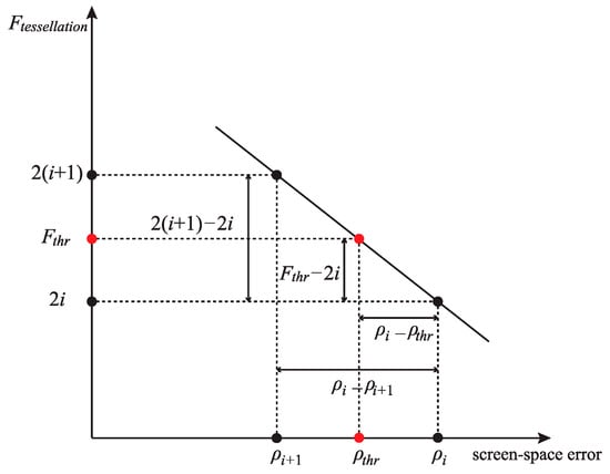
Figure 11. Computation of the tessellation level of ${\rho }_{thr}$.

3.3.2. Hierarchical View Frustum Culling

During navigating, it is possible that only a small part of the terrain model is visible, and the rest is outside the view frustum, especially when the viewpoint is very close to the model. Although OpenGL can cull the geometric model automatically [68], the processing of M-blocks, P-blocks, and DSSs before the automatic culling will expend unnecessary effort on geometries which will not be displayed finally. To reduce the wasting of computing power, we designed a hierarchical view frustum culling scheme (Figure 12). Firstly, the visibility of the M-block is tested using its axis-aligned bounding box (AABB). The M-block is culled when the bounding box is totally outside the view frustum. Secondly, for a visible M-block, the visibility of its four edges is tested and invisible edges will be discarded.

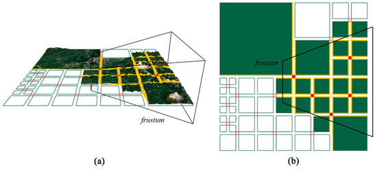
Figure 12. Hierarchical view frustum culling: (a) The empty quads are blocks culled by the frustum. (b) The yellow segments in the frustum represent the block edges that are used to generate DSSs.

4. Experiments and Discussion

Several experiments were conducted to test the visual effect and performance of the algorithm, in two different areas (Area I: Puget Sound and Area II: Grand Canyon [69]). The experimental software system was programmed with C++ and GLSL, and the experiments were conducted on a system with an Intel Xeon E5-2630 2.3 GHz CPU with 16 GB RAM and an NVIDIA Quadro K4000 graphics card.

4.1. Visualization Effect

As shown in Figure 13, two different scenarios of the same region in Area I with different viewpoint parameters are presented to show the effect of the view-dependent terrain reconstruction, where $O$ is the center of the M-block enclosed in the red circle and $\overrightarrow{n}$ is the terrain normal along the positive Z axis. Let $d$ be the distance between the viewpoint and $O$, and $\theta$ be the angle between the view direction and $\overrightarrow{n}$. The values of $d$ and $\theta$ in Figure 13a,b are 725.17, 73.87$°$ and 625.24, 35.46$°$, respectively. These values indicate that although the viewpoint is closer to $O$ in Figure 13b, the M-block has still been retained due to a smaller $\theta$. The two images in Figure 13 show that our multilevel updating scheme is well aware of the roughness of the terrain and the change of viewpoint. Thus, an adaptive tessellation mesh was achieved and the data amount processed in real time was reduced without notably lowering the visual effect.

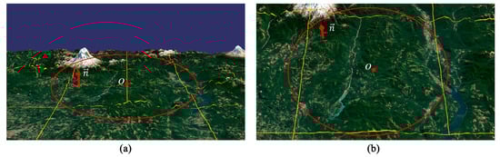
Figure 13. Effect of view direction change (height map size: 1025 × 1025; ${\rho }_{thr}$: 1.0): (a) Four M-blocks in the red circle. (b) The four M-blocks in (a) are replaced by its parent node.

Figure 14 presents some details of how the DSS seamlessly connects adjacent M-blocks. Even if there is a big difference between the tessellation levels on both sides, the DSS can track the moving vertices on the common edges and can connect them in a seamless manner at run time (see the red circles in Figure 14b). From Figure 14b, we can see that the DSSs are well triangulated without any visual artefacts caused by thin triangles. Moreover, the junction of different DSSs is also well-handled by placing a P-block.

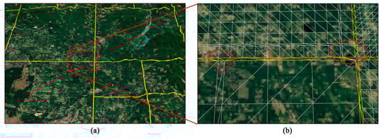
Figure 14. Effect of DSSs: (a) Part of the model that is seamlessly connected by DSSs and (b) Magnified view of the portion enclosed in the red rectangle in (a).

In order to verify the improved visual effect, we compared our method with two other terrain rendering methods. Method I is a quadtree based algorithm using power of two as tessellation levels referring to the study of [9], and Method II is a continuous LOD algorithm dividing the terrain with uniform patterns referring to the study of [60]. Figure 15 presents some frames of a navigation route in Area I along which the viewpoint gradually approaches the terrain model. The height map size here is 1025 × 1025 and screen-space error threshold is 1 (A more vivid presentation of the comparison can be found in the Supplementary Materials). We used the same error control metric for the three methods. Dramatic changes can be found in the first row (Method I), and unnatural changes appear in the middle row (Method II); while there are no popping artefacts in the third row (our method). The reason will be explained later.

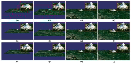
Figure 15. Visual effect comparison in Area I: (a–d) Method I. (e–h) Method II. (i–l) Our method.

The comparison of the three methods is also conducted in Area II (Figure 16). Compared with Area I, Area II is relatively flatter without high peaks. As the viewpoint approaching the terrain model, the three methods have a good effect in gentle regions. The reason is that in the gentle regions without many details, a coarse mesh is enough to meet the requirement of screen-space error threshold, and a more detailed mesh will not bring any improvement to the visual quality. But some small unnatural changes can still be observed in the blue circles along the canyon in Method I and Method II.

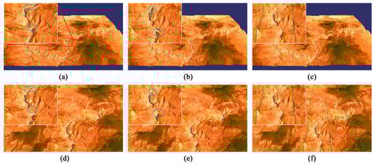
Figure 16. Visual effect comparison in Area II: (a) and (d) for Method I. (b) and (e) for Method II. (c) and (f) for our method.

Figure 17 presents some quantitative evaluation results of the visual effect in Figure 15 and Table 2 shows the corresponding viewpoint positions. The height difference between coarse terrain models and the origin model are calculated as described in Section 1. Besides, based on Figure 17, the Root Mean Squared Error (RMSE) values were computed for the coarse models as shown in Table 3. The popping artefacts can be reflected by the height difference change between coarse models. For example, in Figure 17a, the regions with significant height differences are colored by red (with the biggest RMSE value of 57.72) and the variation in height difference from Figure 17a,b is also obvious (the change of RMSE is 40.62), corresponding with the popping artefact from Figure 15a,b.

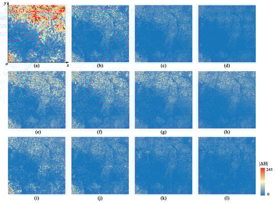
Figure 17. Quantitative evaluation of visual quality: (a–d) Method I. (e–h) Method II. (i–l) Our method.

Table 2. Viewpoint positions in Figure 17: the side length of each height difference map in Figure 17 is 1024 (Column 1 corresponds with the first column in Figure 17 and Column 2 corresponds with the second column in Figure 17 and so on).

	Column 1		Column 2		Column 3		Column 4
	x	y	x	y	x	y	x	y
Viewpoint position	501.1	−1418.3	507.6	−938.8	489.7	−216.6	506.2	106.0

Table 3. RMSE values of coarse models (Column 1 corresponds with the first column in Figure 17 and Column 2 corresponds with the second column in Figure 17 and so on).

	RMSE Values
	Column 1	Column 2	Column 3	Column 4
Method I	57.72	17.10	10.44	6.59
Method II	19.72	14.42	11.35	9.15
Our Method	17.96	12.86	8.53	6.74

Method II divides the terrain into several blocks with equal sizes and each block has a continuous LOD, thus the transition from Figure 17e–h is smoother than Method I. However, Figure 17g shows a greater height difference than Figure 17c,k. This is because the uniform division pattern of Method II limits the adaptive refinement of terrain. This fixed pattern will not change according to the roughness of the terrain at run time. Therefore, unreasonable division may appear. For example, in rugged regions, there may be a sparse division of the terrain, and in flat regions, the terrain may be over-divided.

Method I and our method both employed the quadtree structure to construct adaptive LOD, but as can be seen from Figure 17i–l, there is a slighter variation which reveals the improved visual quality of our method. The reason is that Method I uses $2^n$ for tessellation levels for the purpose of eliminating cracks. However, using fixed discrete tessellation levels prevents the terrain blocks from becoming finer. In our method, with the help of DSS, each M-block can be adjusted independently without considering cracks, and can thus change in a continuous manner to meet the error requirements to the greatest extent. As shown in Figure 18, even with the same quadtree division, the inner meshes of the M-blocks are much finer than those of Method I.

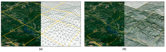
Figure 18. Comparison of meshes of the two methods in Area I (height map size: 1025 × 1025): (a) Method I. (b) Our method.

The influence of the screen-space error threshold on the visual effect was also explored as shown in Figure 19. From Figure 19a–h, some details of the peak disappeared and the quadtree division of the terrain model became coarser with the screen-space error threshold changing from 1 to 8 under the same viewpoint conditions. As described in Section 3.3.1, if ${\rho }_{thr}$ increases, a lower quadtree level and a smaller tessellation level are just able to satisfy the requirement of ${\rho }_{thr}$, which results coarser meshes. Besides, when a bigger ${\rho }_{thr}$ is used, the resulted coarser meshes will not be able to preserve the features in rugged regions, thus the height difference between coarse models and original model will become greater.

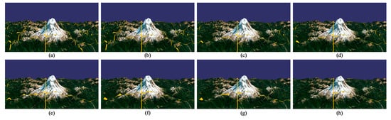
Figure 19. Comparison of visual effect under different screen-space error threshold using our method: The ${\rho }_{thr}$ ranges from 1.0 to 8.0 from (a–h).

4.2. Performance Analysis

As shown in Figure 20a, a 4097 × 4097 height map of Area I is used to test the program performance. As the number of triangles increases, the curve drops rapidly at first and then the frame rate decreases gently, indicating a decline in the influence of data amount on program performance. Besides rendering the primitives of the terrain model, there are some updating tasks that need to be executed in each frame. With the terrain model becoming finer, the multilevel model splits into deeper levels and there will be more M-blocks and DSSs to deal with at run time, which will also decrease the frame rate. In this test scene, the number of triangles reached the maximum value of 2.35 million with a frame rate of 32 fps. For a more complex area, this number could be greater since more M-blocks, P-blocks, and DSSs are generated, but the frame rate will decrease. Nevertheless, most of the time, the terrain rendering program can run smoothly.

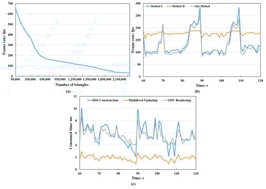
Figure 20. Efficiency test using a 4097 × 4097 height map with a 1280 × 960 viewport: (a) Frame rates and data amount. (b) Performance comparison. (c) Consumed time of different stages in our method.

For further evaluation of the program performance, the frame rate of our method was compared with Method I and Method II in Figure 20b. We tested the three methods using the same roaming route. At 70, 89, and 109 s, sudden changes are observed in the curves of Method I and our method. At these moments, the viewpoint moved from flat regions to rugged regions by panning the terrain model, resulting in a sudden drop of frame rate. Method II uses a fixed and uniform terrain division manner which will not change at run time, therefore, there is no updating operations in CPU, and a higher frame rate is achieved. In Method I and our method, a quadtree structure was used and adjusted in real-time to realize the adaptive tessellation of terrain. A quadtree with deeper levels has more updating tasks than a quadtree with lower levels, which resulted the fluctuations of frame rate in Method I and our method. The curve of Method I is a little higher than that of our method. We can ascertain the reason for this difference. In our method, a continuous LOD adjustment of M-Blocks is achieved by introducing the DSS. However, at the same time, the work of DSS generation needs to be done in every frame, which costs some extra time. It is noteworthy, though, that at the same moment, the data amount rendered in our method is greater than that of Method I, which means a more detailed terrain model.

Figure 20c shows the consumed time of different stages in our method. In the entire framework, the Multilevel Updating stage (including quadtree updating, visibility testing and tessellation level computing) took up approximately 2 ms, whereas the time spent on the DSS Construction and GPU Rendering varied from 2 ms to 10 ms and 4 ms to 10 ms respectively. In general, the cost of DSS construction is largely dependent on the complexity and number of DSSs. By using a multithread strategy, the construction of DSSs is efficient and an acceptable average frame rates (125 fps) could be achieved.

As for the CPU usage, our method is higher than that of Method I and II due to the updating tasks in CPU (including multilevel updating and DSS construction) as shown in Table 4. Method I and our method need to store the object-space errors and MBD data is also required in our method. Although the rendered terrain model may contain millions of triangles, the vertex data of all the three methods are still small because most of the triangles are generated in the GPU tessellation stage. The vertex data of our method is more than that of Method I and II because the DSSs are constructed in CPU, which need extra space to store the vertices. Besides, most of the video memory is used to store height maps and textures.

Table 4. CPU usage and memory consumption of the three methods using a 4097 × 4097 height map in Area I.

	CPU Usage (avg.)	Main Memory			Video Memory
		Object-Space Error	MBD	Vertex Data	Height Map	Texture
Method I	5.2%	700 KB	—	15 KB	18.5 MB	23.0 MB
Method II	4.9%	—	—	200 KB
Our Method	12.4%	700 KB	18 KB	1.2 MB

5. Conclusions

We presented a real-time terrain rendering method based on GPU tessellation, which can significantly reduce the visual popping artefacts and improve the reality of terrain models. With the help of the stitching structure, DSS, the tessellation levels of terrain blocks can be adjusted in a continuous manner without restricting the terrain blocks in several limited levels. Using a multithread strategy, the tasks of DSS edge tessellation and DSS triangulation are executed concurrently. Thus, DSSs can be generated at run time to fill the gaps between adjacent blocks. By considering the regularity of DSSs, our triangulation algorithm is able to eliminate the artefacts caused by thin triangles. Moreover, by applying a hierarchical view frustum culling strategy, unnecessary blocks and DSSs are culled before the auto culling of OpenGL, which saves significant computational resources and improves the efficiency of our method.

There are still some aspects that are worthy of inclusion in future work. First, a dynamic partitioning method such as KD-tree can be used to replace the quadtree division. By dividing the terrain according to the roughness of the local regions, mountain areas and flat areas can avoid being in the same terrain block. Thus the object-space error computed for the terrain block will be more accurate. Second, the task of DSS triangulation could be moved to the GPU. In our current implementation, each step in the triangulation process must consider the global condition of the DSS. However, when using the GPU pipeline, the whole geometry is broken into separate primitives and there is no communication between them. Thus, designing a new indexing scheme or vertex dependency rules may be an alternative solution [70]. Third, the proposed multilevel terrain model is constructed based on the quadtree division of a whole height map. However, for height maps that cannot be loaded completely into the main memory, using a series of independent terrain tiles is necessary. Therefore, scheduling strategy and crack avoidance techniques for terrain tiles will be studied in the future. Finally, reducing the preprocessing time of computing the object space error will further improve the practicability of our method.

References

- Zhe, G.; Yandian, Z.; Yangyu, F.; Siqiang, H.; Shu, L.; Yi, W. Multi-thread block terrain dynamic scheduling based on three-dimensional array and Sudoku. Multimed. Tools Appl. 2018, 77, 5819–5835. [Google Scholar] [CrossRef]
- Luebke, D.; Reddy, M.; Cohen, J.D.; Varshney, A.; Watson, B.; Huebner, R. Level of Detail for 3D Graphics; Morgan Kaufmann: Burlington, MA, USA, 2003. [Google Scholar]
- Wagner, D. Terrain geomorphing in the vertex shader. In ShaderX2: Shader Programming Tips & Tricks with DirectX; Wordware Publishing: Plano, TX, USA, 2004; pp. 18–32. [Google Scholar]
- Goanghun, K.; Nakhoon, B. A height-map based terrain rendering with tessellation hardware. In Proceedings of the 2014 International Conference on IT Convergence and Security (ICITCS), Beijing, China, 28–30 October 2014. [Google Scholar]
- Azuma, D.I.; Wood, D.N.; Curless, B.; Duchamp, T.; Salesin, D.H.; Stuetzle, W. View-dependent refinement of multiresolution meshes with subdivision connectivity. In Proceedings of the 2nd International Conference on Computer Graphics, Virtual Reality, Visualisation and Interaction in Africa, Cape Town, South Africa, 3–5 February 2003; ACM: New York, NY, USA; pp. 69–78. [Google Scholar] [CrossRef]
- Losasso, F.; Hoppe, H. Geometry clipmaps: Terrain rendering using nested regular grids. In ACM Transactions on Graphics (TOG); ACM: New York, NY, USA, 2004; pp. 769–776. [Google Scholar] [CrossRef]
- Cozzi, P.; Ring, K. 3D Engine Design for Virtual Globes; AK Peters: Natick, MA, USA; CRC Press: Boca Raton, FL, USA, 2011. [Google Scholar]
- Lee, E.S.; Lee, J.H.; Shin, B.S. Vertex relocation: A feature-preserved terrain rendering method for pervasive computing environments. Multimed. Tools Appl. 2016, 75, 14057–14073. [Google Scholar] [CrossRef]
- Rui, Z.; Ke, L.; Weiguo, P.; Shuangfeng, D. GPU-based real-time terrain rendering: Design and implementation. Neurocomputing 2016, 171, 1–8. [Google Scholar] [CrossRef]
- Song, G.; Yang, H.; Ji, Y. Geometry clipmaps terrain rendering using hardware tessellation. IEICE Trans. Inf. Syst. 2017, E100-D, 401–404. [Google Scholar] [CrossRef]
- Gibson, S.F.F. Beyond volume rendering: Visualization, haptic exploration, and physical modeling of voxel-based objects. In Visualization in Scientific Computing ’95; Springer: Vienna, Austria, 1995; pp. 10–24. [Google Scholar] [CrossRef]
- Taosong, H. Volumetric virtual environments. J. Comput. Sci. Technol. 2000, 15, 37–46. [Google Scholar] [CrossRef]
- Dey, R.; Doig, J.G.; Gatzidis, C. Procedural feature generation for volumetric terrains using voxel grammars. Entertain. Comput. 2018, 27, 128–136. [Google Scholar] [CrossRef]
- Koca, Ç.; Güdükbay, U. A hybrid representation for modeling, interactive editing, and real-time visualization of terrains with volumetric features. Int. J. Geogr. Inf. Sci. 2014, 28, 1821–1847. [Google Scholar] [CrossRef]
- D’Oliveira, R.B.D.; Apolinário, A.L., Jr. Procedural Planetary Multi-Resolution Terrain Generation for Games. 2018. Available online: https://arxiv.org/pdf/1803.04612.pdf (accessed on 15 February 2019).
- Geiss, R. Generating Complex Procedural Terrains Using the GPU. 2007. Available online: https://developer.nvidia.com/gpugems/GPUGems3/gpugems3_ch01.html (accessed on 15 February 2019).
- Parberry, I. Designer worlds: Procedural generation of infinite terrain from real-world elevation data. J. Comput. Graph. Tech. 2014, 3, 74–85. [Google Scholar]
- Smelik, R.M.; Kraker, K.J.D.; Groenewegen, S.A.; Tutenel, T.; Bidarra, R. A survey of procedural methods for terrain modelling. In Proceedings of the CASA Workshop on 3D Advanced Media in Gaming and Simulation, Amsterdam, The Netherlands, 16 June 2009; pp. 25–34. [Google Scholar]
- Mahdavi-Amiri, A.; Alderson, T.; Samavati, F. A survey of digital earth. Comput. Graph. 2015, 53, 95–117. [Google Scholar] [CrossRef]
- Kumler, M.P. An intensive comparison of Triangulated Irregular Networks (TINs) and Digital Elevation Models (DEMs). Cartographica: Int. J. Geogr. Inf. Geovis. 1994, 31, 1–99. [Google Scholar] [CrossRef]
- Schroeder, W.J.; Zarge, J.A.; Lorensen, W.E. Decimation of triangle meshes. Siggraph 1992, 92, 65–70. [Google Scholar] [CrossRef]
- Cohen-Or, D.; Levanoni, Y. Temporal Continuity of Levels of Detail in Delaunay Triangulated Terrain; IEEE: Piscataway, NJ, USA, 1996; pp. 37–42. [Google Scholar] [CrossRef]
- Cignoni, P.; Puppo, E.; Scopigno, R. Representation and visualization of terrain surfaces at variable resolution. Vis. Comput. 1997, 13, 199–217. [Google Scholar] [CrossRef]
- El-Sana, J.; Varshney, A. Generalized view-dependent simplification. In Computer Graphics Forum; Blackwell Publishers Ltd.: Oxford, UK; Boston, MA, USA, 1999; Volume 18, pp. 83–94. [Google Scholar]
- Garland, M.; Heckbert, P.S. Surface simplification using quadric error metrics. In Proceedings of the 24th Annual Conference on Computer Graphics and Interactive Techniques, Los Angeles, CA, USA, 3–8 August 1997; ACM Press: Boston, MA, USA, 1997; pp. 209–216. [Google Scholar]
- Yang, B.; Li, Q.; Shi, W. Constructing multi-resolution triangulated irregular network model for visualization. Comput. Geosci. 2005, 31, 77–86. [Google Scholar] [CrossRef]
- De Floriani, L.; Puppo, E. Hierarchical triangulation for multiresolution surface description. ACM Trans. Graph. 1995, 14, 363–411. [Google Scholar] [CrossRef]
- Hoppe, H. Smooth view-dependent level-of-detail control and its application to terrain rendering. In Proceedings of the Visualization ’98, Research Triangle Park, NC, USA, 18–23 October 1998; pp. 35–42. [Google Scholar] [CrossRef]
- Hoppe, H. View-dependent refinement of progressive meshes. In Proceedings of the 24th Annual Conference on Computer Graphics and Interactive Techniques, Los Angeles, CA, USA, 3–8 August 1997; ACM Press: Boston, MA, USA, 1997; pp. 189–198. [Google Scholar] [CrossRef]
- Bertilsson, E.; Goswami, P. Dynamic Creation of Multi-resolution Triangulated Irregular Network. In Proceedings of the SIGRAD, Visby, Sweden, 23–24 May 2016; pp. 1–8. [Google Scholar]
- Rebollo, C.; Remolar, I.; Chover, M.; Ramos, J.F. A comparison of multiresolution modelling in real-time terrain visualization. In Computational Science and Its Applications–ICCSA 2004, Proceedings of the International Conference on Computational Science and Its Applications, Assisi, Italy 14–17 May 2004; Springer: Berlin/Heidelberg, Germany, 2004; pp. 703–712. [Google Scholar]
- De Boer, W.H. Fast Terrain Rendering Using Geometrical Mipmapping. 2000. Available online: http://www.flipcode.org/ archives/ article_geomipmaps.pdf (accessed on 15 February 2019).
- Asirvatham, A.; Hoppe, H. Terrain rendering using GPU-based geometry clipmaps. GPU Gems 2005, 2, 27–46. [Google Scholar]
- Van Den Hurk, S.; Yuen, W.; Wünsche, B. Real-time terrain tendering with incremental loading for interactive terrain modelling. In Proceedings of the International Conference on Computer Graphics Theory and Applications (GRAPP 2011), Vilamoura Algarve, Portugal, 5–7 March 2011; pp. 181–186. [Google Scholar]
- Schneider, J.; Boldte, T.; Westermann, R. Real-time editing, synthesis, and rendering of infinite landscapes on GPUs. Vis. Model. Vis. 2006, 2006, 145–152. [Google Scholar]
- Johanson, C. Real-time Water Rendering: Introducing the Projected Grid Concept. Master’s Thesis, Lund University, Lund, Sweden, 2004. [Google Scholar]
- Livny, Y.; Sokolovsky, N.; Grinshpoun, T.; El-Sana, J. A GPU persistent grid mapping for terrain rendering. Vis. Comput. 2008, 24, 139–153. [Google Scholar] [CrossRef]
- Evans, W.; Kirkpatrick, D.; Townsend, G. Right-triangulated irregular networks. Algorithmica 2001, 30, 264–286. [Google Scholar] [CrossRef]
- Lindstrom, P.; Pascucci, V. Visualization of large terrains made easy. In Proceedings of the Conference on Visualization, San Diego, CA, USA, 21–26 October 2001; IEEE Computer Society: Washington, DC, USA; pp. 363–371. [Google Scholar]
- Pajarola, R.; Gobbetti, E. Survey of semi-regular multiresolution models for interactive terrain rendering. Vis. Comput. 2007, 23, 583–605. [Google Scholar] [CrossRef]
- Pajarola, R. Large scale terrain visualization using the restricted quadtree triangulation. In Proceedings of the Visualization ‘98, Research Triangle Park, NC, USA, 18–23 October 1998; pp. 18–23. [Google Scholar] [CrossRef]
- Duchaineau, M.; Wolinsky, M.; Sigeti, D.E.; Miller, M.C.; Aldrich, C.; Mineev-Weinstein, M.B. ROAMing terrain: Real-time optimally adapting meshes. In Proceedings of the 8th Conference on Visualization, Phoenix, AZ, USA, 24 October 1997; IEEE Computer Society Press: Los Alamitos, CA, USA; pp. 81–88. [Google Scholar]
- Lindstrom, P.; Koller, D.; Ribarsky, W.; Hodges, L.F.; Faust, N.; Turner, G.A. Real-time, continuous level of detail rendering of height fields. In Proceedings of the 23rd Annual Conference on Computer Graphics and Interactive Techniques, New Orleans, LA, USA, 4–9 August 1996; pp. 109–118. [Google Scholar] [CrossRef]
- Röttger, S.; Heidrich, W.; Slusallek, P.; Seidel, H.P. Real-time generation of continuous levels of detail for height fields. J. WSCG 1998, 6, 1–3. [Google Scholar]
- Levenberg, J. Fast view-dependent level-of-detail rendering using cached geometry. In Proceedings of the IEEE Visualization, Boston, MA, USA, 27 October–1 November 2002; pp. 259–265. [Google Scholar]
- Pajarola, R.; Antonijuan, M.; Lario, R. QuadTIN: Quadtree based triangulated irregular networks. In Proceedings of the Conference on Visualization, Boston, MA, USA, 27 October–1 November 2002; IEEE Computer Society: Washington, DC, USA; pp. 395–402. [Google Scholar]
- Lario, R.; Pajarola, R.; Tirado, F. Hyperblock-quadtin: Hyper-block quadtree based triangulated irregular networks. In Proceedings of the IASTED International Conference on Visualization, Imaging and Image Processing (VIIP 2003), Benalmadena, Spain, 8–10 September 2003; pp. 733–738. [Google Scholar]
- Velho, L. Using semi-regular 4–8 meshes for subdivision surfaces. J. Graph. Tools 2000, 5, 35–47. [Google Scholar] [CrossRef]
- Cignoni, P.; Ganovelli, F.; Gobbetti, E.; Marton, F.; Ponchio, F.; Scopigno, R. Planet-sized batched dynamic adaptive meshes (P-BDAM). In Proceedings of the 14th IEEE Visualization, Washington, DC, USA, 22–24 October 2003; IEEE Computer Society: Washington, DC, USA; pp. 20–27. [Google Scholar] [CrossRef]
- Cignoni, P.; Ganovelli, F.; Gobbetti, E.; Marton, F.; Ponchio, F.; Scopigno, R. BDAM-Batched dynamic adaptive meshes for high performance terrain visualization. Comput. Graph. Forum 2003, 22, 505–514. [Google Scholar] [CrossRef]
- Baumann, K.; Döllner, J.; Hinrichs, K.; Kersting, O. A hybrid, hierarchical data structure for real-time terrain visualization. In Proceedings of the Computer Graphics International, Canmore, AB, Canada, 7–11 June 1999; pp. 85–92. [Google Scholar] [CrossRef]
- Paredes, E.G.; Bóo, M.; Amor, M.; Döllner, J.; Bruguera, J.D. GPU-based visualization of hybrid terrain models. In Proceedings of the International Conference on Computer Graphics Theory and Applications (GRAPP 2012), Rome, Italy, 24–26 February 2012; pp. 254–259. [Google Scholar]
- Yilmaz, T.; Güdükbay, U.; Akman, V. Modeling and visualization of complex geometric environments. In Geometric Modeling: Techniques, Applications, Systems and Tools; Springer: Dordrecht, The Netherlands, 2004; pp. 3–30. [Google Scholar]
- Bóo, M.; Amor, M. Dynamic hybrid terrain representation based on convexity limits identification. Int. J. Geogr. Inf. Sci. 2009, 23, 417–439. [Google Scholar] [CrossRef]
- Bóo, M.; Amor, M.; Döllner, J. Unified hybrid terrain representation based on local convexifications. Geoinformatica 2007, 11, 331–357. [Google Scholar] [CrossRef]
- Paredes, E.G.; Bóo, M.; Amor, M.; Bruguera, J.D.; Döllner, J. Extended hybrid meshing algorithm for multiresolution terrain models. Int. J. Geogr. Inf. Sci. 2012, 26, 771–793. [Google Scholar] [CrossRef]
- Paredes, E.G.; Bóo, M.; Amor, M.; Bruguera, J.D.; Döllner, J. Hybrid terrain rendering based on the external edge primitive. Int. J. Geogr. Inf. Sci. 2016, 30, 1095–1116. [Google Scholar] [CrossRef]
- OpenGL Wiki. 2017. Available online: http://www.khronos.org/opengl/wiki_opengl/indexphp?title=Tessellation&oldid= 14135 (accessed on 15 February 2019).
- Nießner, M.; Keinert, B.; Fisher, M.; Stamminger, M.; Loop, C.; Schäfer, H. Real-time rendering techniques with hardware tessellation. Comput. Graph. Forum 2015, 35, 113–137. [Google Scholar] [CrossRef]
- Fernandes, A.R.; Oliveira, B. GPU tessellation: We still have a lod of terrain to cover. In OpenGL Insights; CRC Press: Boca Raton, FL, USA, 2012; pp. 145–162. [Google Scholar]
- Cantlay, I. DirectX 11 Terrain Tessellation. 2011. Available online: https://developer.download.nvidia.cn/assets/gamedev/files/sdk/11/TerrainTessellation_WhitePaper.pdf (accessed on 15 February 2019).
- Yusov, E.; Shevtsov, M. High-performance terrain rendering using hardware tessellation. J. Wscg 2011, 19, 85–92. [Google Scholar]
- Ulrich, T. Rendering massive terrains using chunked level of detail control. In Proceedings of the 29th International Conference on Computer Graphics and Interactive Techniques, San Antonio, TX, USA, 21–26 July 2002. [Google Scholar]
- Livny, Y.; Kogan, Z.; El-Sana, J. Seamless patches for GPU-based terrain rendering. Vis. Comput. 2009, 25, 197–208. [Google Scholar] [CrossRef][Green Version]
- HyeongYeop, K.; Hanyoung, J.; Chang-Sik, C.; JungHyun, H. Multi-resolution terrain rendering with GPU tessellation. Vis. Comput. 2015, 31, 455–469. [Google Scholar] [CrossRef]
- Mikhaylyuk, M.V.; Timokhin, P.Y.; Maltsev, A.V. A method of Earth terrain tessellation on the GPU for space simulators. Progr. Comput. Softw. 2017, 43, 243–249. [Google Scholar] [CrossRef]
- Segal, M.; Akeley, K. The OpenGL Graphics System: A specification (Version 4.5 (Core Profile)—29 June 2017). 2017. Available online: https://www.khronos.org/registry/OpenGL/specs/gl/glspec45.core.pdf (accessed on 15 February 2019).
- Shreiner, D.; Sellers, G.; Kessenich, J.; Licea-Kane, B. Introduction to OpenGL. In OpenGL Programming Guide: The Official Guide to Learning OpenGL, 8th ed.; Version 4.3; Addison-Wesley Professional: Boston, MA, USA, 2013; pp. 1–32. [Google Scholar]
- USGS and The University of Washington. Model: Puget Sound. 2018. Available online: https://www.cc.gatech.edu/projects/large_models/ps.html (accessed on 15 February 2019).
- Ripolles, O.; Ramos, F.; Puig-Centelles, A.; Chover, M. Real-time tessellation of terrain on graphics hardware. Comput. Geosci. 2012, 41, 147–155. [Google Scholar] [CrossRef]
© 2019 by the authors. Licensee MDPI, Basel, Switzerland. This article is an open access article distributed under the terms and conditions of the Creative Commons Attribution (CC BY) license (http://creativecommons.org/licenses/by/4.0/).