Machine Learning Algorithms for Automatic Lithological Mapping Using Remote Sensing Data: A Case Study from Souk Arbaa Sahel, Sidi Ifni Inlier, Western Anti-Atlas, Morocco

Abstract

Remote sensing data proved to be a valuable resource in a variety of earth science applications. Using high-dimensional data with advanced methods such as machine learning algorithms (MLAs), a sub-domain of artificial intelligence, enhances lithological mapping by spectral classification. Support vector machines (SVM) are one of the most popular MLAs with the ability to define non-linear decision boundaries in high-dimensional feature space by solving a quadratic optimization problem. This paper describes a supervised classification method considering SVM for lithological mapping in the region of Souk Arbaa Sahel belonging to the Sidi Ifni inlier, located in southern Morocco (Western Anti-Atlas). The aims of this study were (1) to refine the existing lithological map of this region, and (2) to evaluate and study the performance of the SVM approach by using combined spectral features of Landsat 8 OLI with digital elevation model (DEM) geomorphometric attributes of ALOS/PALSAR data. We performed an SVM classification method to allow the joint use of geomorphometric features and multispectral data of Landsat 8 OLI. The results indicated an overall classification accuracy of 85%. From the results obtained, we can conclude that the classification approach produced an image containing lithological units which easily identified formations such as silt, alluvium, limestone, dolomite, conglomerate, sandstone, rhyolite, andesite, granodiorite, quartzite, lutite, and ignimbrite, coinciding with those already existing on the published geological map. This result confirms the ability of SVM as a supervised learning algorithm for lithological mapping purposes.

1. Introduction

Lithology is closely related to many important issues such as geological disasters, mineral storage, and oil reservoirs. Satellite remote-sensing data and advances in digital image processing (DIP) techniques provided a new impulse to the development of lithological mapping. Spectral data from space and airborne sensors were widely applied to geological mapping, including lithological discrimination [1,2,3,4,5,6,7,8], structural mapping [9], hydrothermal alteration [10,11,12], and economic mineral deposits [13,14,15,16,17]. Because of their cost effectiveness, especially in mapping inaccessible areas [4,18,19,20] and in the production of small-scale maps, remote-sensing methods provide a good alternative to traditional field work [21]. In geological areas, remote sensing is based on differences in the physical and chemical properties of rocks. Due to these disparities, the different types of rocks reflect the electromagnetic energy in different wavelengths, which allows the identification of the spectral characteristics of the mineralogy of the rock. This is the basis of spectrum-based approaches for mapping or automated lithological classification. Regarding the classification techniques, machine learning algorithms (MLAs), a sub-domain of artificial intelligence, aim to automatically extract information from data, through statistical or non-probabilistic approaches. This classification technique is divided into two types: (i) unsupervised classification, which classifies the rock type based solely on the spectral information without being assisted by training zones and without the process resulting in spectral clustering by an iterative technique [19,22,23,24]; and (ii) supervised classification, which consists of assigning groups of identical pixels to classes that correspond to each type of rock by comparing the pixels with each other and with those whose lithology is known. The advances in supervised image classification techniques based on MLAs improved geological studies using remote-sensing data. The classification algorithms that were successfully applied in geological mapping include the maximum likelihood classifier (MLC) [25,26], naïve Bayes (NB) [27,28], artificial neural networks (ANNs) [27,29,30,31], k-nearest neighbors (K-NN) [26,27], and random forests (RF) [29,32]. In this study, an image classification algorithm considering support vector machines (SVMs) is used as an empirical method (a data-driven technique). SVMs are supervised learning algorithms, which are considered as heuristic algorithms, based on statistical learning theory [33]. This method was further developed in various supervised classification applications during the last decade [34], and was previously employed in lithological mapping [21,35,36,37,38]. This method also proved to be more accurate in the field of remote sensing than other classification methods [39]. For this study, SVM was applied to perform an automated lithological classification (lithological mapping) of the region of Souk Arbaa Sahel belonging to the Sidi Ifni inlier located in southern Morocco (Western Anti-Atlas) using remote-sensing data, namely Landsat 8 Operational Land Imager (OLI) data and a digital elevation model (DEM) of ALOS/PALSAR with 12.5-m spatial resolution. Several image pre-processing and processing techniques were applied to process the Landsat 8 data in order to generate products that should improve lithological information. SVM performance was evaluated by the accuracy of the classification on independent validation samples, such as similarity with a regional geological map and Google Earth^® data. This work was carried out in five stages: (i) data preprocessing, (ii) visual interpretation of different lithological units, (iii) automatic lithological mapping by SVM, (iv) accuracy evaluation, and (v) assessment.

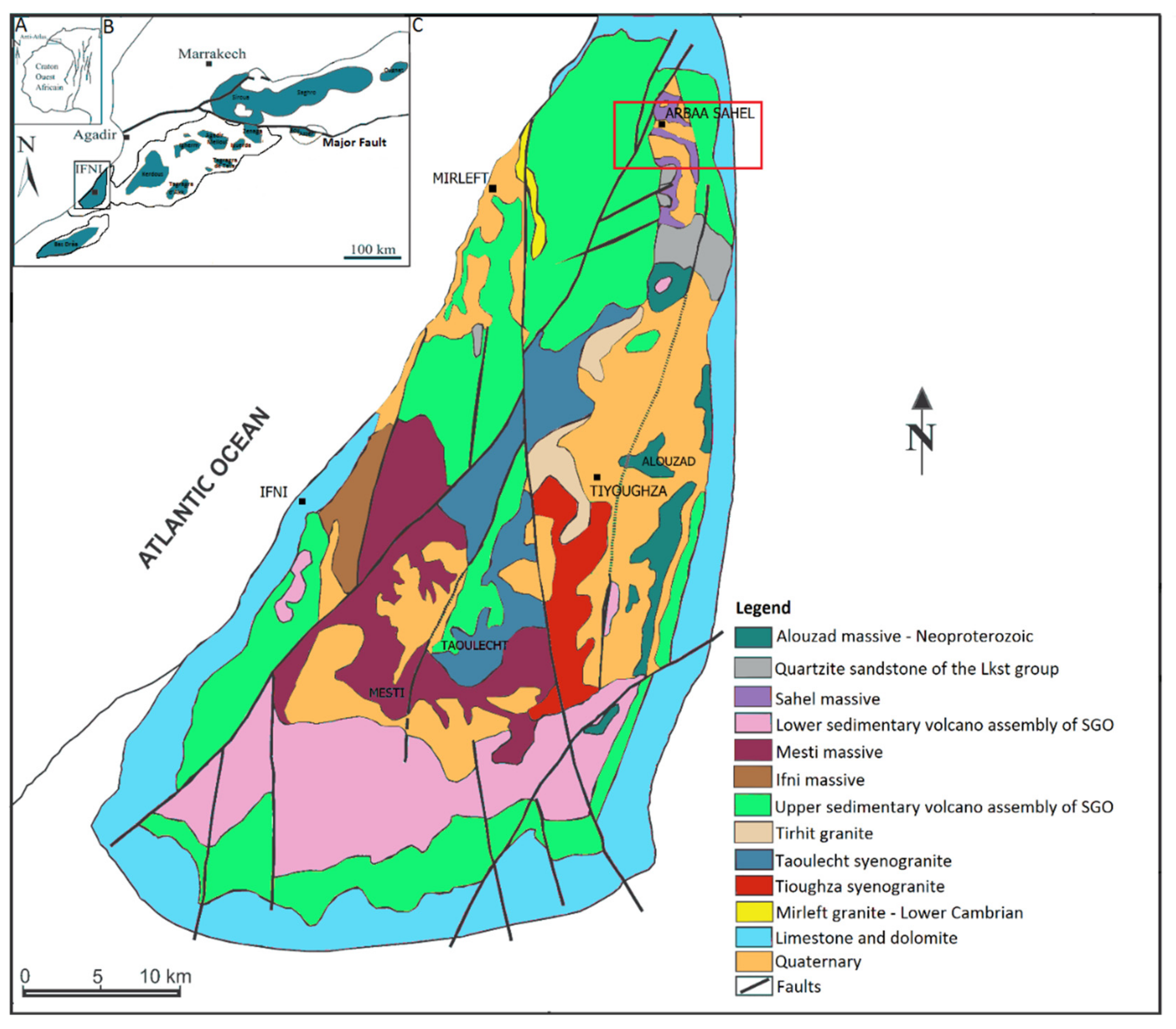
2. Study Area Description

2.1. Geographical Location

The Sidi Ifni inlier is located about 150 km south of Agadir city, and it is the most western inlier of the Anti-Atlas (Figure 1B). Its natural boundaries are formed by the Tiznit plain in the north, the Tleta Akhssas plateau in the east, the Noun wadi in the south, and the Atlantic Ocean in the west.

The Souk Arbaa Sahel study area is in the northern part of the Sidi Ifni inlier (Figure 1C); this region delimits an area of approximately 50 km². It is bordered by the meridians 9°49′30′′ and 9°58′30′′ west and the parallels 29°39′ and 29°35′30′′ north.

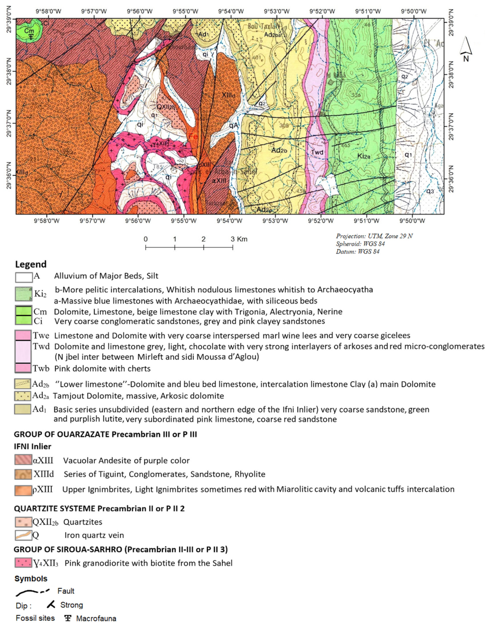
2.2. Geological Context

The Moroccan Anti-Atlas is located in the northern part of the West African craton (WAC) (Figure 1A), where Proterozoic terranes outcrop in the form of inliers within a Neoproterozoic to Paleozoic cover [40]. The substratum of Anti-Atlas inliers was structured by two main Precambrian orogenic events: (i) the Eburnean and (ii) the Pan-African [41,42,43,44]. The presently outcropping Precambrian inliers (Figure 1B) are basement folds that formed during the Variscan deformation [45]. The Sidi Ifni inlier is situated in the western edge of Anti-Atlas. It is composed (Figure 2) of a Paleoproterozoic granitic basement and a Neoproterozoic cover [46,47] intruded by Neoproterozoic granites with Rb/Sr ages situated between 689 ± 20 Ma and 541 ± 8 Ma [40,48,49,50,51]. The Neoproterozoic cover constitutes a quarzitic sandstone sedimentary series followed without unconformity with a volcano-sedimentary series, the bode series belong to a super Ouarzazate group (SOG) [40]. Early Cambrian limestones overcome this series [52].

3. Materials and Methods

A Landsat OLI image and a digital elevation model (DEM) derived from ALOS (Advanced Land Observing Satellite)/PALSAR (Phased Array Type L-Band Synthetic Aperture Radar) were considered in this study. Several image processing programs were used, namely QGIS 3.0, SNAP 6.0, and SAGA GIS 6.3.0. Satellite image pre-processing and processing techniques such as radiometric calibration, reflectance conversion, and vegetation suppression were applied to achieve the main purposes of the study.

3.1. Landsat OLI Data

A cloud-free level L1TP (standard terrain corrected) Landsat OLI image (Path/Row 203/39) was obtained for free through the United States Geological Survey (USGS) Earth Resources Observation and Science Center (EROS). It was acquired on 3 February 2018 for the Souk Arbaa Sahel region. The image map projection is UTM zone 29 N, considering the WGS-84 datum.

The Landsat OLI sensor (multispectral instrument) collects image data in nine bands (visible, near-infrared, and shortwave infrared bands). These data have a high-performance radiometer signal-to-noise ratio (SNR), enabling 12-bit data quantization to enable more bits for better land-cover characterization. Landsat 8 OLI data have 30-m spatial resolution for bands 1 to 7 and band 9. The band 8 (panchromatic) spatial resolution is 15 m (

Table 1. Spectral and spatial resolution of the Landsat Operational Land Imager (OLI) bands.

Landsat OLI-Bands	Spatial Resolution	Wavelength (µm)
Band 1—coastal aerosol	30 m	0.43–0.45
Band 2—blue	30 m	0.45–0.51
Band 3—green	30 m	0.53–0.59
Band 4—red	30 m	0.64–0.67
Band 5—near-infrared (NIR)	30 m	0.85–0.88
Band 6—shortwave infrared (SWIR) 1	30 m	1.57–1.65
Band 7—SWIR 2	30 m	2.11–2.29
Band 8—panchromatic	15 m	0.50–0.68
Band 9—cirrus	30 m	1.36–1.38

). Bands 1 and 9 were designed for atmospheric correction (they were excluded from the lithological classification performed in this study).

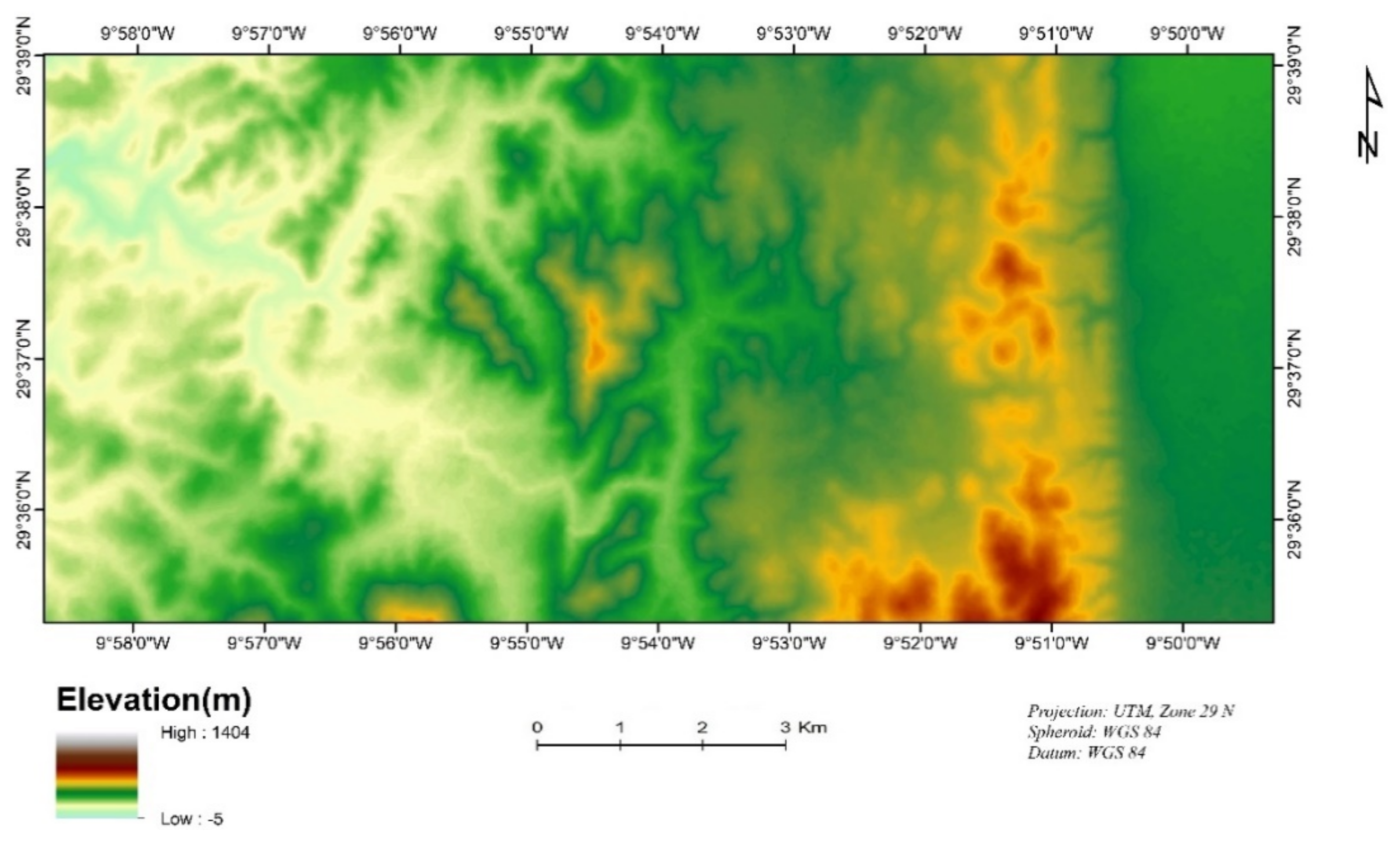
3.2. Digital Elevation Model

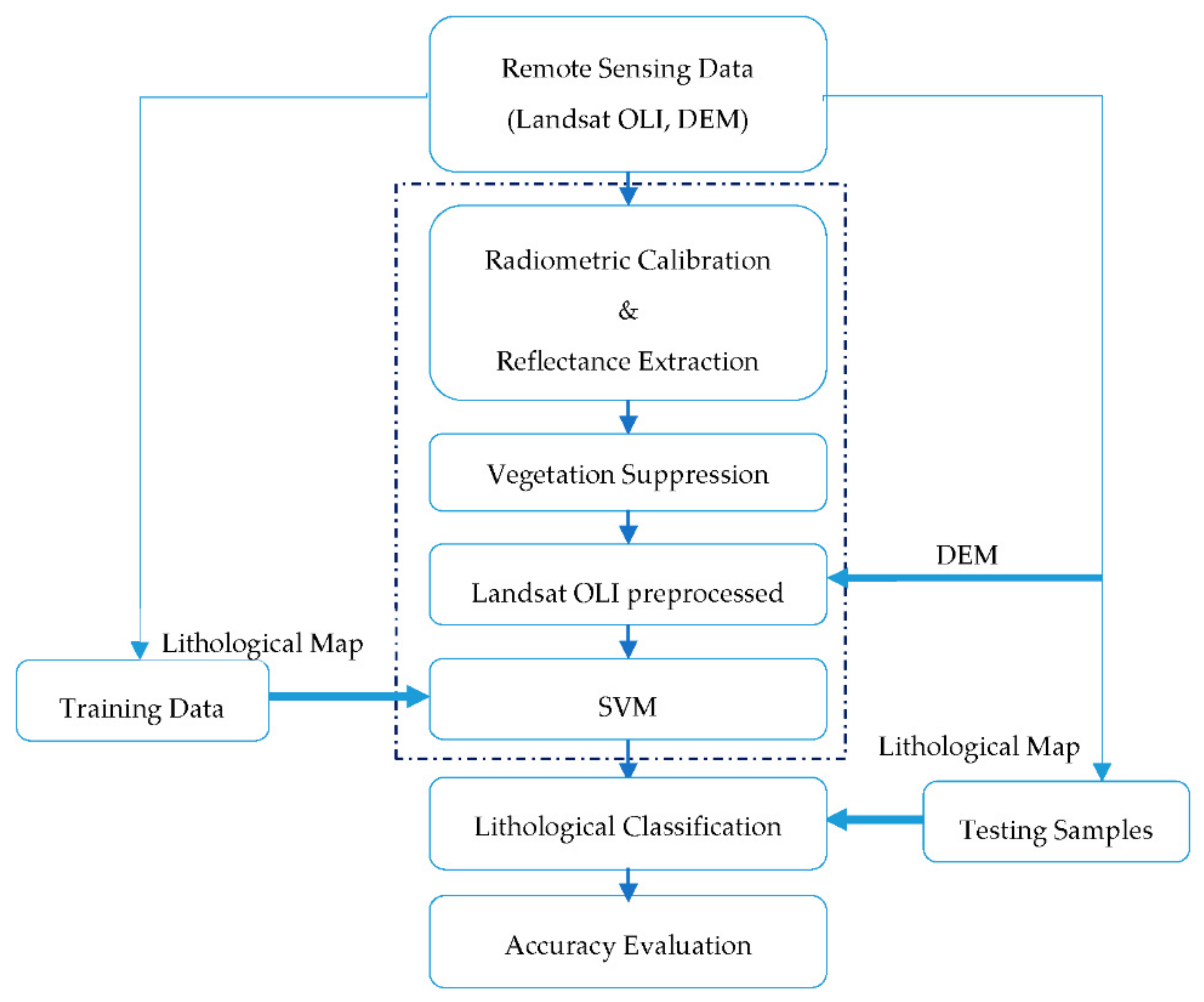
A DEM obtained from ALOS/PALSAR with 12.5-m spatial resolution was used for terrain characterization (Figure 3). These data were obtained with no cost from the National Aeronautics and Space Administration (NASA).

3.3. Methods

In the present study, the methodology used consisted of processing Landsat 8 OLI data and integrating it into the DEM, which provides geomorphological and geological information below the surface by extracting geomorphometric variables (e.g., slope, curvature, and surface roughness), in order to generate products with better lithological information. The local morphometric terrain parameters of slope, curvature, and roughness were derived from the DEM of ALOS/PALSAR. The Basic Terrain Analysis function of SAGA geographic information system (GIS) software was used to produce slope and curvature maps using a moving 3 × 3 pixel neighborhood. The surface roughness was computed using the Terrain Analysis function of the QGIS software using a 3 × 3 pixel window neighborhood. The SVM’s performance was assessed by the accuracy of the classification on independent test samples. Figure 4 illustrates the methodology followed in a sequence diagram. QGIS and SNAP were used for data pre-processing (layer stack, subset, radiometric calibration, surface reflectance conversion, vegetation suppression, and geomorphometric variables). SAGA GIS was also used in the classification step.

3.4. Pre-Processing of Remote-Sensing Data

3.4.1. Radiometric Calibration and Reflectance Conversion

Landsat-8 OLI image bands were converted from digital format (DN) to radiance (L_λ) and top-of-atmosphere (TOA) reflectance (ρ_λ) according to Equations (1) and (2), respectively. We followed the methodology summarized on the USGS website [53].

$$L_{\lambda }=\left(\frac{L_{\mathrm{MAX}}-L_{\mathrm{MIN}}}{Q_{\mathrm{calmax}}-Q_{\mathrm{calmin}}}\right)\left(Q_{\mathrm{cal}}-Q_{\mathrm{calmin}}\right)+L_{\mathrm{MIN}},$$

(1)

$${\rho }_{\lambda }=\left(\frac{\pi \ast L_{\lambda }\ast d^2}{ESU{N}_{\lambda }\ast \cos \theta }\right),$$

(2)

where λ is the band number, L is the spectral radiance at the sensor aperture, L_MAX is the spectral radiance that is scaled to Q_calmax, L_MIN is the spectral radiance that is scaled to Q_calmin, Q_calmax is the maximum quantized calibrated pixel value (corresponding to L_MAX) in DN (65535), Q_calmin is the minimum quantized calibrated pixel value (corresponding to L_MIN) in DN (1), and Q_cal is the quantized calibrated pixel value in DN [54]. All these parameters can be found in the metadata file (.MTL) which accompanied the Landsat OLI images. Furthermore, ρ_λ is the TOA reflectance for each band, d² is the inverse squared relative earth–sun distance, ESUN_λ is the mean exoatmospheric solar irradiance, and θ is the solar zenith angle in degrees.

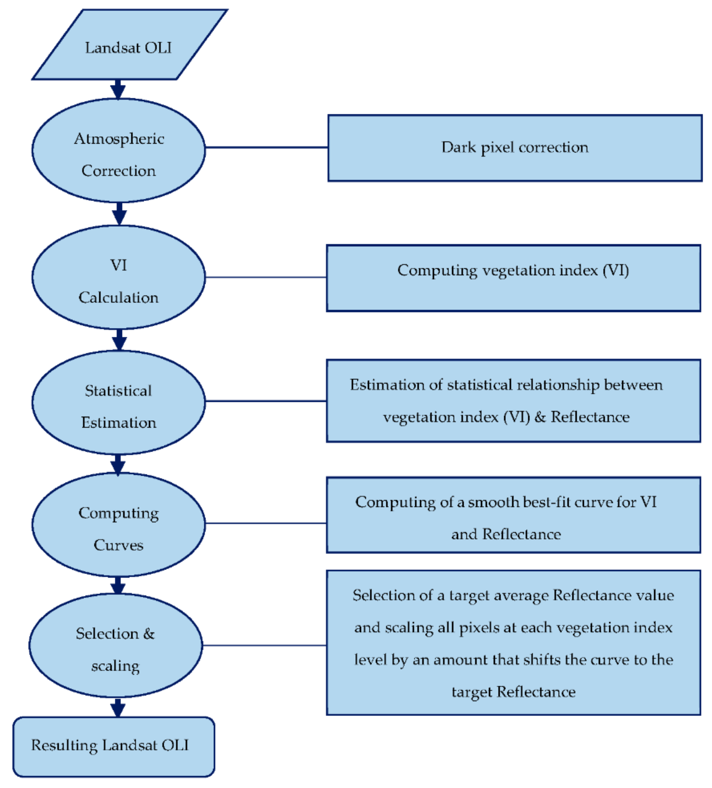
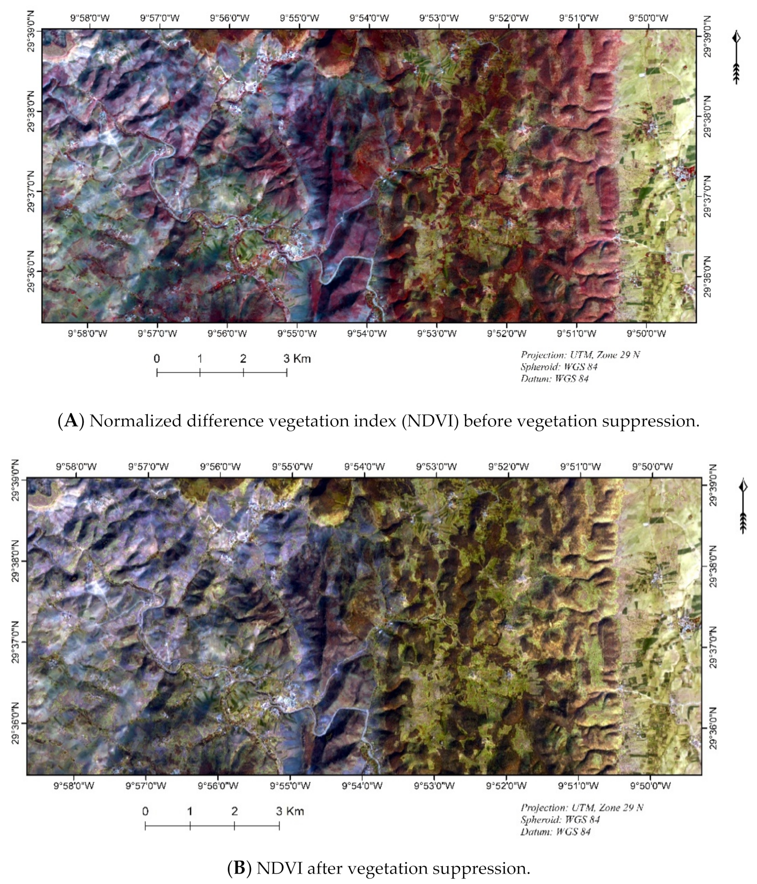
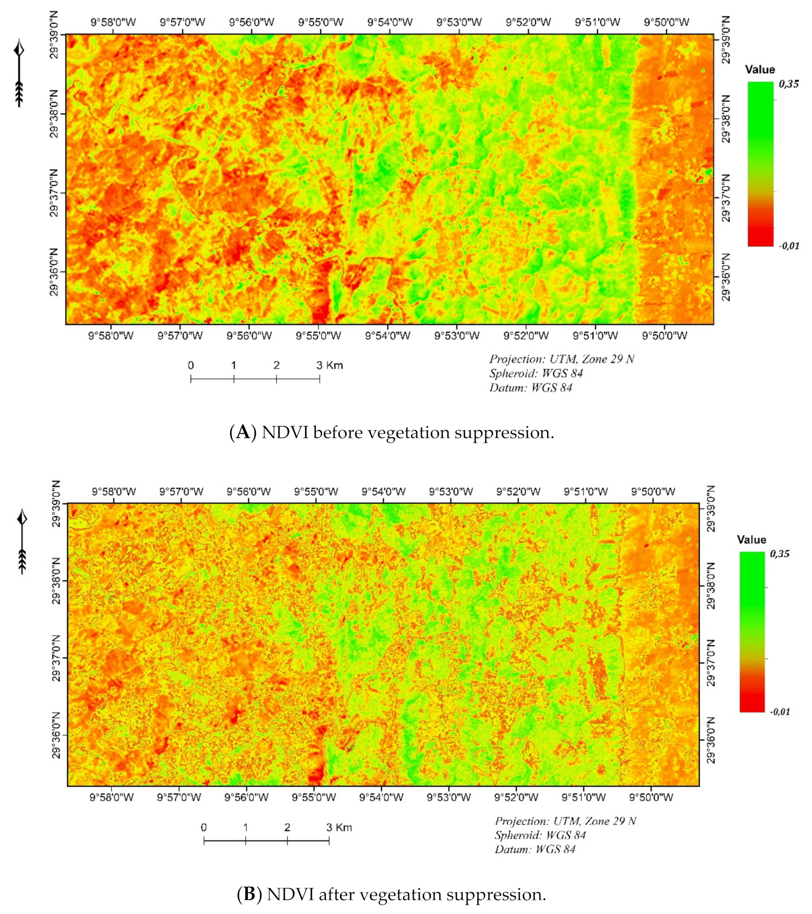
3.4.2. Vegetation Suppression Using the Forced Invariance Method

The spectral response of a rock is influenced by several factors, including the heterogeneity of the chemical and mineralogical composition of the rock at the sub-pixel level, the land-cover type, and, most importantly, the extent and nature of the vegetation cover. The presence of vegetation cover masks the spectral signatures of the underlying geological substrate, making remote lithological mapping more complex [55,56]. To improve geological information, it is, therefore, important to suppress the spectral response of the overlying vegetation cover. The forced invariance method (FIM) is a means of enhancing multispectral remotely sensed imagery for lithologic interpretation, proposed by Crippen and Blom (2001) [57]. It is assumed to decorrelate the vegetative component of the total signal on a pixel-by-pixel basis for each band by computing the relationship of each input band with the vegetation index. It is based on information from red and near-infrared bands of the sensors without requiring any knowledge of lithological composition of the scene. Figure 5 illustrates the FIM [56,58].

The FIM was successfully applied in the geology field using hyper- and multispectral data [58]. The performance of the FIM approach was checked using two criteria: the false color image (by applying visual analysis) and the normalized difference vegetation index (NDVI). It can be observed that the original image (Figure 6A) was dominated by vegetation, whereas, in the treated image (Figure 6B), the red hue was not evident. Another criterion involved using the NDVI. It is apparent that the NDVI values also decreased considerably by comparing Figure 7A,B.

3.5. Training and Testing Samples

The former geological map illustrated (Figure 2) was used to select training and testing samples for the lithological classes. The training and testing samples corresponding to ten lithological units were carefully selected based on the texture properties and distributions of these ten lithological units, as shown in Figure 2. We selected a total of 2980 pixels for the ten lithological units, representing about 1.34% of the whole study area. The training datasets were directly used as input in the SVM classifier. In addition, according to the geological map (Figure 2), 500 randomly distributed ground-truth points in the study area were selected as the testing dataset.

Table 2. The training and testing samples for lithological units.

Lithological Unit	Training Samples (Pixels)	Testing Samples
Silt, alluvium (SA)	396	68
Limestone (L)	228	51
Dolomite, limestone (DL)	456	42
Conglomerate, sandstone, rhyolite (CSR)	386	55
Andesite (A)	377	42
Dolomite (D)	238	59
Granodiorite (G)	455	45
Quartzite (Q)	79	41
Sandstone, lutite, limestone (SLL)	260	45
Ignimbrite (I)	105	52

shows the number of training and testing samples for each of lithological unit.

3.6. Lithological Mapping by SVM

SVMs represent one of the most popular algorithms in the field of machine learning and pattern recognition [59], which attracted increasing interest in the field of remote sensing [60,61] because of their ability to successfully manage small sets of learning data, often producing higher classification accuracy when compared with traditional methods. The success of SVMs is justified by the solid theoretical foundations that support it. They make it possible to address a wide range of problems, including classification. SVMs were proposed by Vapnik [33], based on the theory of statistical learning and the principle of minimizing structural risk. It is intended to solve complicated class distributions in spectral data [60,61].

SVM is a particularly well-suited method for processing very large datasets. SVM classifiers are initially two-class linear classifiers, based on a criterion to maximize the separation margin of the two classes. Indeed, it is a question of determining a hyperplane with a maximum distance to the nearest learning examples (support vectors). The hyperplane that maximizes this distance, called the “margin”, is the optimal separator hyperplane. The robustness of SVM classifiers comes from the introduction of a penalty for classification errors in the criterion to be optimized, a penalty that ensures a better ability to generalize. In non-separable linear cases, SVM find a hyperplane while incorporating a parameter C, which adjusts the penalty associated with misclassifying support vectors. High values of C generate more complex prediction functions in order to misclassify as few support vectors as possible by way of a high penalty on error [62,63]. The objective function must be modified to incorporate this penalty term for wide-margined decision boundaries with misclassified support vectors as shown below.

Minimize

$$\Vert \mathrm{w}{\Vert }^2+\mathrm{C}{{\displaystyle \sum }}_{\mathrm{i}=1}^{\mathrm{N}}{\mathsf{\epsilon }}_{\mathrm{i}},$$

(3)

subject to

$$yi\left(w.xi+b\right)\ge 1-\epsilon i,\epsilon i>0,\hspace{1em}i=1,\dots ,N,$$

(4)

where w is a coefficient vector that determines the orientation of the hyperplane in the feature space, b is the offset of the hyper plane from the origin, and $\epsilon i$ is the positive slack variables which represent the distance to misclassified support vectors from their respective marginal hyperplanes. For non-linear cases, SVM uses an implicit transformation of input variables via a kernel function [64,65],

$$k\left(xi,xj\right)=\phi \left(xi\right)\phi \left(xj\right),$$

(5)

which returns the inner product between the positions of pairwise compared input variables (xi and xj) in variable space. The kernel function allows SVM to handle non-linear relationships efficiently between classes and variables by projecting samples from the original d-dimensional variable space into a potentially infinite dimensional kernel space [62]. In this case, the form of the decision function is written as

$$f:f\left(x\right)=sgn\left(w.\phi \left(x\right)\right)+b.$$

(6)

Kernel function selection is essential to the success of SVM training and classification accuracy. Several common kernel functions for the SVM include linear kernel (LN), polynomial kernel (PL), radial basis function (RBF) kernel, and sigmoid kernel (SIG). According to Zhu et al. [66], the most important advantage of using RBF is that it has good interpolation capabilities. Therefore, in this study, the kernel function RBF was selected.

SVM performance depends on the kernel parameter choice. For the radial basis function, the penalty parameter and the gamma kernel width are the two parameters that need to be determined. The gamma parameter controls the degree of non-linearity of the SVM model, as long as the penalty parameter controls the level of error to be tolerated in the training data. A large value for penalty parameters will result in some training errors, while a small value for penalty parameters will generate a larger margin and, thus, increase the number of training errors [67]. According to Yang [68], RBF-SVM represents the best kernel type when the penalty parameter is at 100 and the gamma parameter in the kernel function is the inverse of the band numbers in the input. In the present work, the penalty parameter was set to 100, and the gamma parameter in the kernel function was the inverse of the band number of the Landsat OLI DEM dataset, i.e., 0.16 [26,35]. The RBF-SVM was performed in SAGA GIS 6.3.0 software and all data were scaled between −1 and 1 prior to their input into the SVM.

3.7. Lithological Mapping by Artificial Neural Network

ANN is a computer algorithm based on the biological neural system. ANN is widely used to solve complex problems in different application fields, including pattern recognition, identification, classification, and control systems. The ANN classifier is an artificial intelligence technique that attempts to simulate how people classify patterns, learn tasks, and solve problems [69]. It consists of a number of simple processing units named nodes [70]. The nodes are linked according to a specified architecture by weighted connections. The ANN classifier in this study contained three layers: an input layer, a middle layer (i.e., hidden layer), and an output layer. Each layer of the ANN classifier consists of one or more nodes that are adjusted to obtain the most reasonable output through the iterative experiment [69]. In this research, a multi-layer feed-forward ANN method was employed with the Landsat OLI DEM dataset for lithological classification using SAGA GIS 6.3.0 software. A logistic function of the logarithmic function was used to configurate ANN. The training contribution threshold and the training momentum field were set at 0.9. The number of hidden layer neurons was 1. The training rate field and the training root-mean-square (RMS) exit criteria were set to 0.2 and 0.1, respectively [26].

3.8. Accuracy Evaluation

The classification performance was quantitatively assessed by computing the overall (OA), user (UA), and producer (PA) accuracies from the confusion matrix and the Kappa coefficient (K) [71]. The OA is the ratio between the total number of correct pixels and the total number of pixels in the error matrix, whereas the UA includes commission errors and PA includes omission errors related to individual classes [35,55,72]. The Kappa coefficient is a statistical measure that represents the accord between classified map and reference data [73]. It considers the possibility of agreements occurring by chance in a random classification. For this reason, it is considered a more reliable measure of classification accuracy [72,74]. Kappa values range from 0 to 1, with values close to 1 indicating little uncertainty in the class identity of a pixel, while values close to 0 indicate high classification uncertainty. In this study, the test samples were randomly selected according to the visual interpretation of geological map.

4. Results

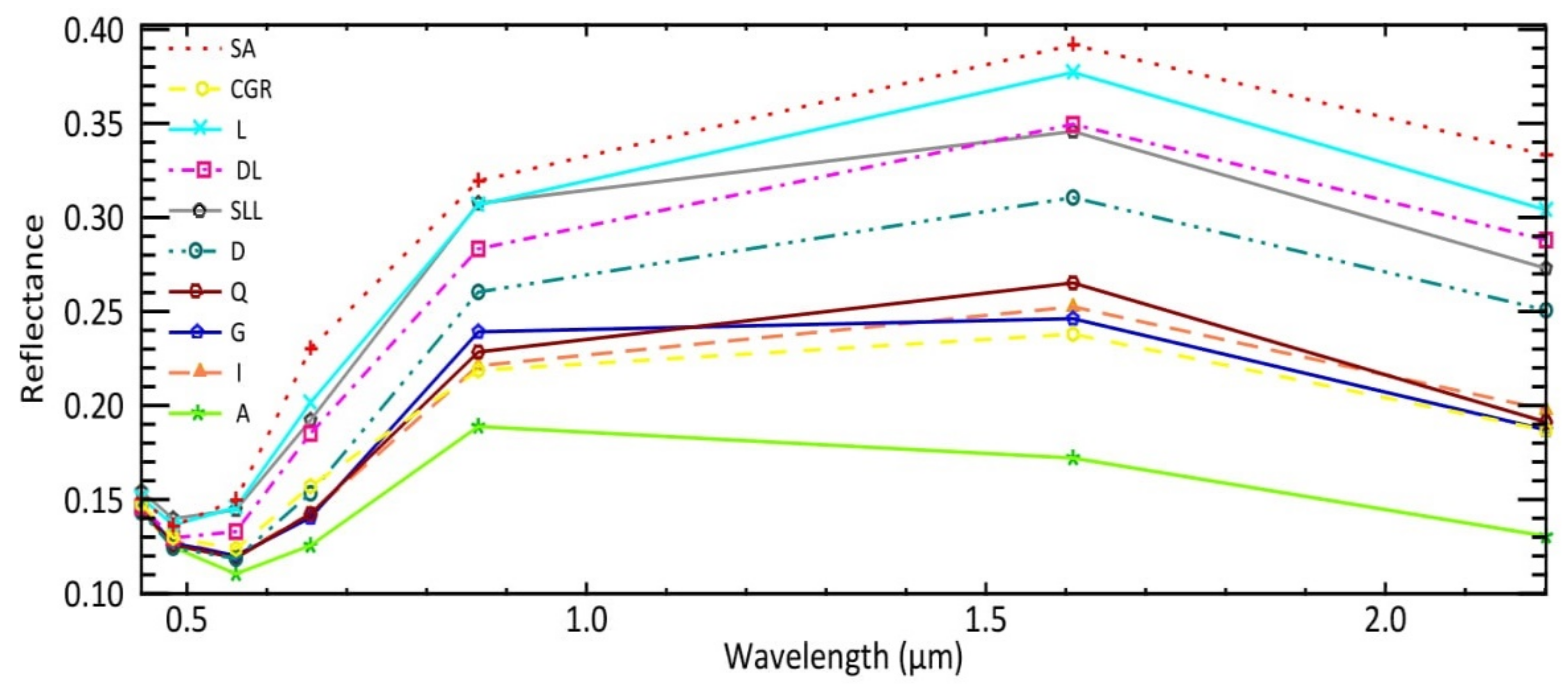
4.1. Training Area Statistics

The average values of all samples for Landsat OLI reflectance for each class are shown in Figure 8. The average overall reflectance of silt and alluvium was higher than other rock types, while the average overall reflectance of andesite rocks was lower than other rock types (Figure 8). For the other classes, the average overall reflectances of the limestone, the sandstone, lutite, and limestone, and the dolomite and limestone classes were higher than the dolomite, granodiorite, quartzite, and ignimbrite. The maximum average reflectance registered in the Landsat OLI data for the Souk Arbaa Sahel area was ~0.39 for the silt and alluvium (SA) class at the 1.57–1.65-μm wavelength region of the Landsat OLI reflectance data. The minimum average reflectance registered in the ASTER data was ~0.11 for the andesite class at the 0.53–0.59-μm wavelength region of the Landsat OLI reflectance data (Figure 8).

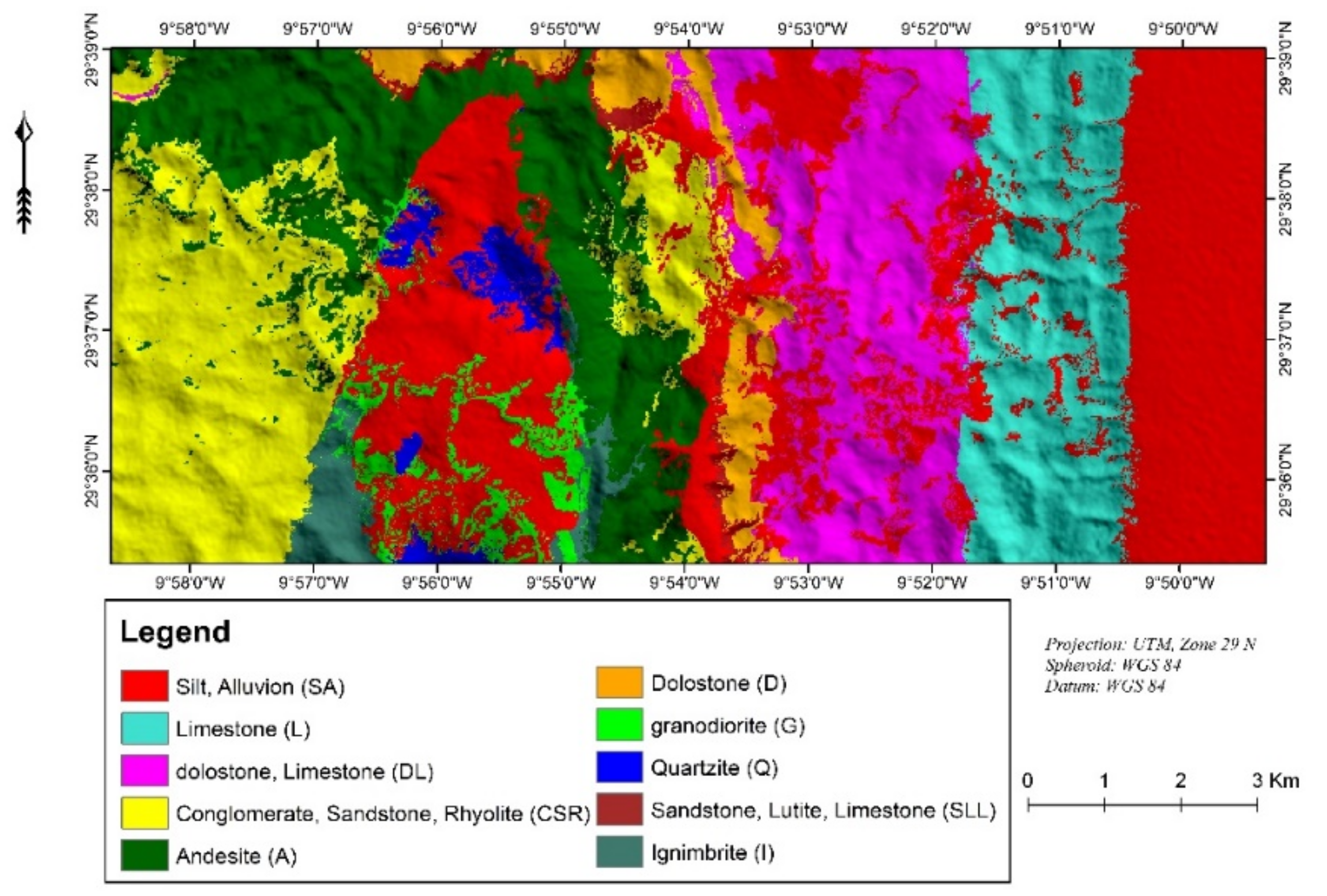
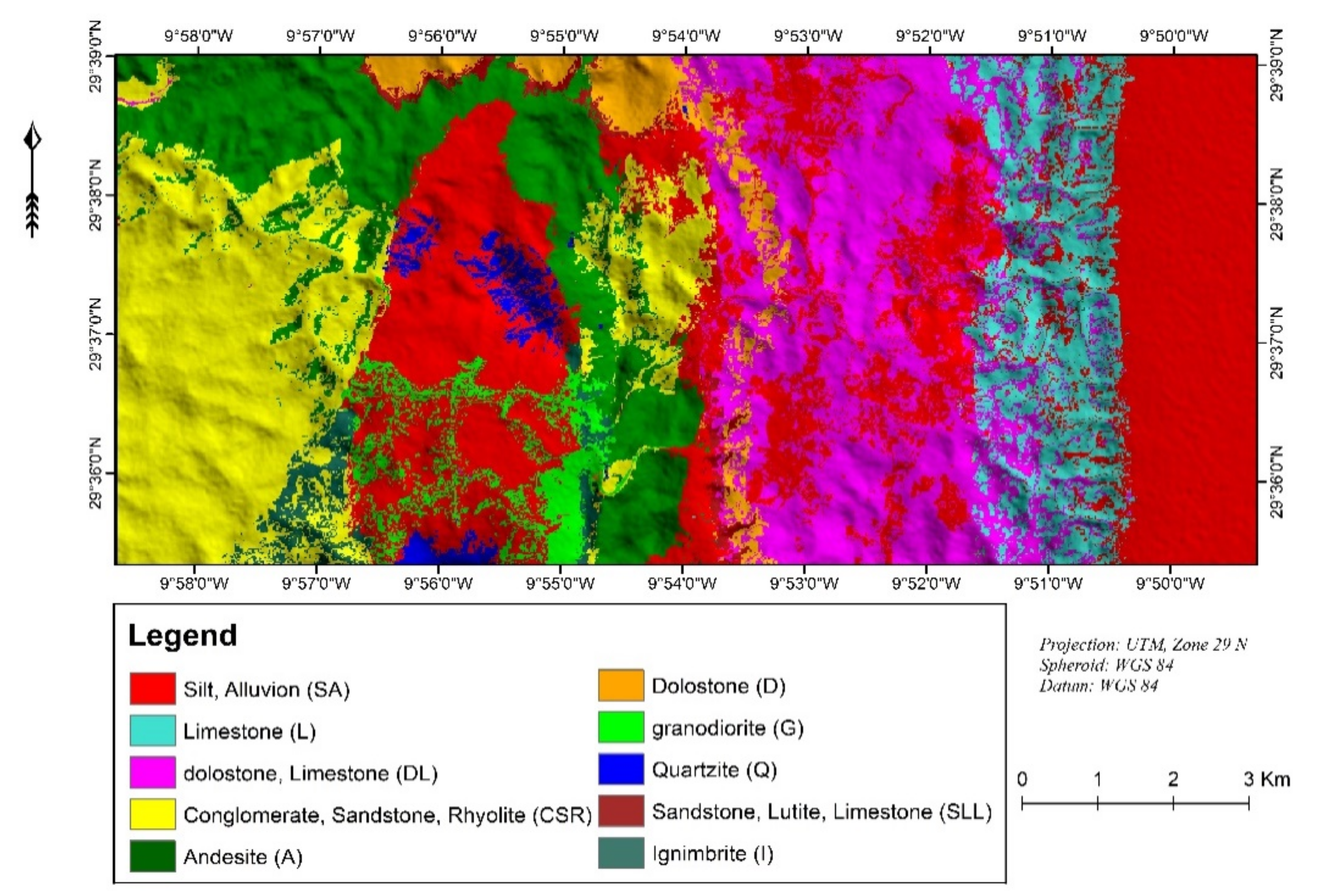
4.2. Lithological Classification Map

The Landsat OLI lithological classification map after the post-classification processing is shown in Figure 9. Post-classification processing was conducted to improve heterogeneity in the region of the same type of rock by eliminating noisy pixels. We used as a post-classification processing technique a majority filter of 3 × 3 pixels in the classification image to filter out parasitic pixels. More details were provided in the Landsat OLI data classification result. From the perspective of the overall visual effect, the Landsat OLI lithological classification map was more similar to the geological map (Figure 2). The ten lithological units defined were distinguished well.

In comparison with the geological map of Tiznit 1/100,000 (Figure 2), the map of the lithological classification obtained via the SVM method applied to the Landsat OLI image showed some agreement. Facies spread over large areas show this agreement well, while there were no smaller facies, such as the large quartz vein. At the level of the wadis, river sediments were detected, corresponding to the leaching products of the andesitic facies crossed by the wadis, which crossed conglomerate, sandstone, and rhyolite formations and areas with silt and alluvial leaching deposits on the edges of the wadis crossing the dolomites.

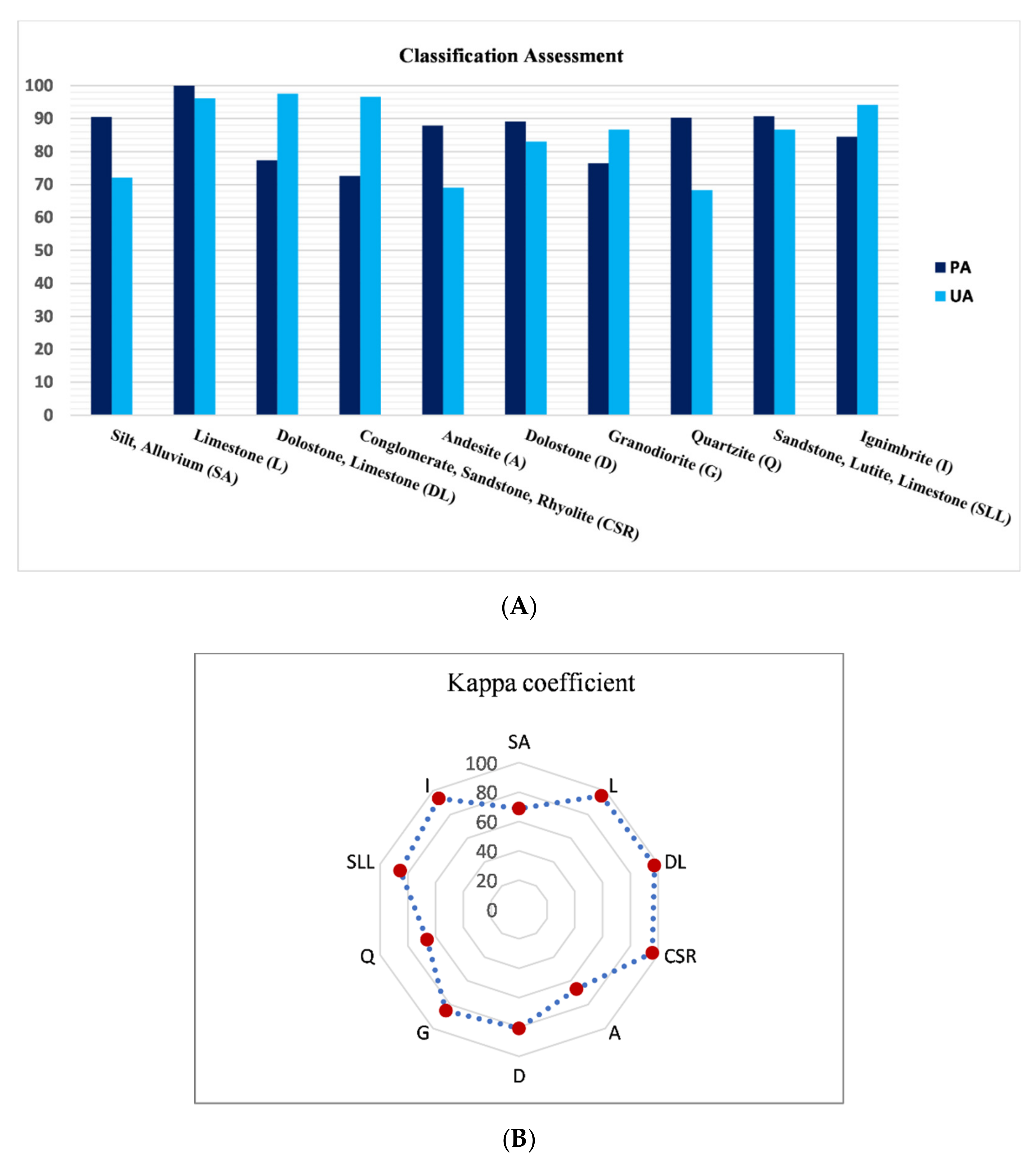
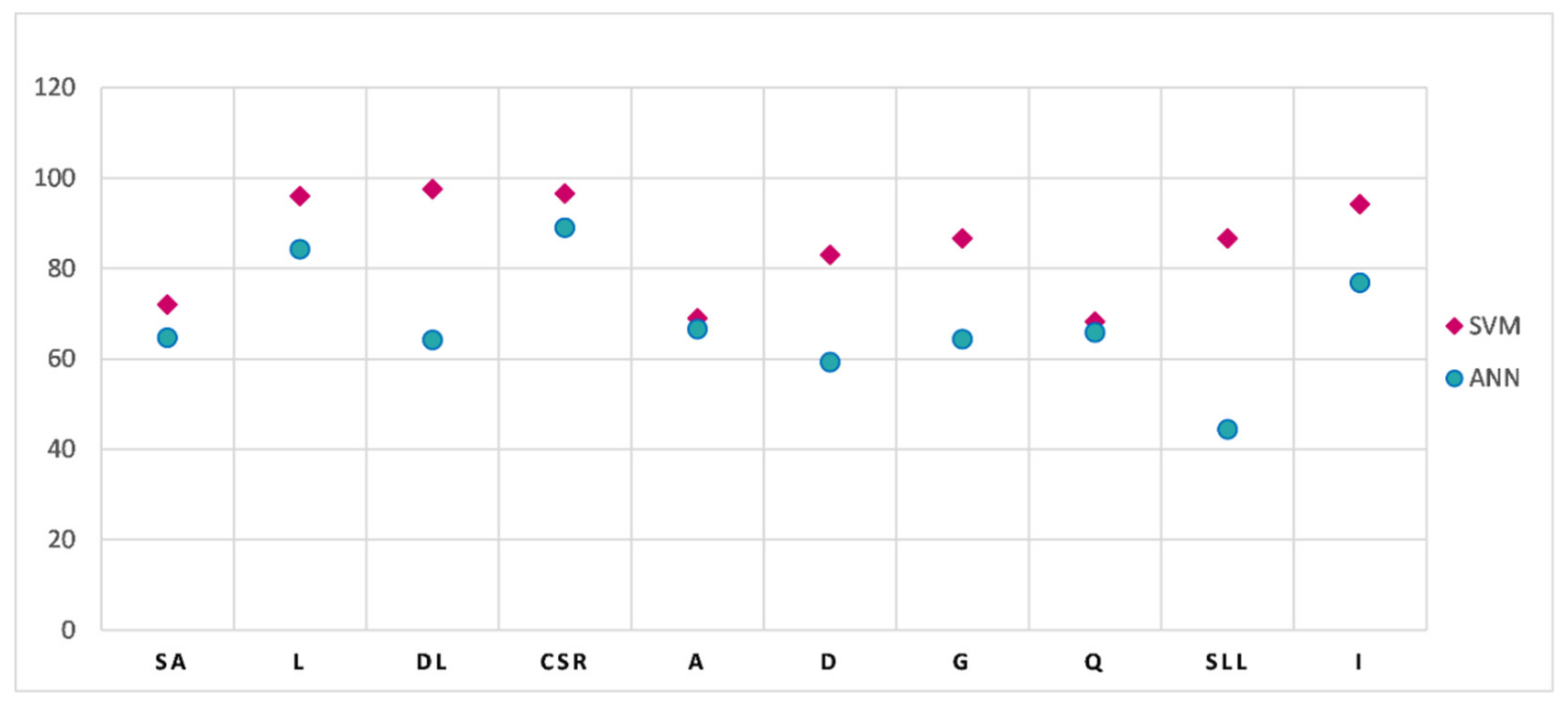
4.3. Classification Accuracy

To evaluate the classification accuracy, samples from the geological map of the study area were selected. Five hundred (500) samples from the reference map were randomly selected to compute the classification accuracy.

Table 3. Error matrix and statistical measures for support vector machine (SVM). The error matrix was summarized based on the statistical measures: producer accuracy (PA), user accuracy (UA), overall accuracy (OA), and the Kappa coefficient (κ).

Reference
	SA	L	DL	CSR	A	D	G	Q	SLL	I	∑	PA	UA
Silt, Alluvium (SA)	49	0	4	4	2	0	7	0	1	1	68	90.47%	72.06%
Limestone (L)	1	49	1	0	0	0	0	0	0	0	51	100%	96.08%
Dolomite, Limestone (DL)	0	0	41	0	0	1	0	0	0	0	42	77.36%	97.62%
Conglomerate, Sandstone, Rhyolite (CSR)	0	0	0	53	2	0	0	0	0	0	55	72.60%	96.36%
Andesite (A)	0	0	0	13	29	0	0	0	0	0	42	87.88%	69.05%
Dolomite (D)	0	0	7	0	0	49	0	0	3	0	59	89.09%	83.05%
Granodiorite (G)	0	0	0	0	0	0	39	3	0	3	45	76.74%	86.67%
Quartzite (Q)	3	0	0	1	0	0	4	28	0	5	41	90.32%	68.29%
Sandstone, Lutite, Limestone (SLL)	1	0	0	0	0	5	0	0	39	0	45	90.70%	86.67%
Ignimbrite (I)	0	0	0	2	0	0	1	0	0	49	52	84.48%	94.23%
∑	54	49	53	73	33	55	51	31	43	58	500	OA	85%
												K	83.29%

shows the PA, UA, OA, and Kappa coefficient (K) for the lithology classification using the SVM method. The OA and the Kappa coefficient were 85% and 83.29%, respectively. The OA was estimated using the contingency error matrix to assess validation (Table 3). The PA and UA for all the lithological units identified are illustrated in Figure 10A. The limestone (L), sandstone, lutite, and limestone (SLL), silt and alluvium (SA), and quartzite classes presented the best PA (>90.00%), and the limestone (L) and conglomerate, sandstone, and rhyolite (CSR) classes showed the best UA (>96.00%). Lower PA classification was achieved for the conglomerate, sandstone, and rhyolite (CSR) (72.60%) class, while the lowest UA obtained was 68.29%, for the quartzite (Q) class. According to Figure 10B, the lithological classes of dolomite and limestone (DL), conglomerate, sandstone, and rhyolite (CSR), limestone (L), and ignimbrite (I) presented the highest Kappa coefficients with 97.34%, 95.74%, 95.65%, and 93.47%, respectively, while quartzite presented the lowest Kappa coefficient with 66.2%.

5. Discussion

MLAs are attracting increasing interest in the field of remote sensing as an approach to geological mapping. Although multispectral and hyperspectral data are widely used for lithological discrimination and classification, it is difficult to obtain appropriate data for geological mapping because of the high cost and complexity of the treatment [26]. Therefore, the combination of multispectral data with textural data and lithological classification characteristics is very effective in achieving good results.

In this research, SVM was evaluated for lithological classification in an area with moderate vegetation coverage. It was shown that the SVM method achieved good results in most rock units in the study area, apart from the quartz vein. The SVM allowed the levels of the wadis and river sediments to be detected, corresponding to the leaching products of the andesitic facies crossed by the wadis, which crossed the conglomerate, sandstone, and rhyolite formations and areas with silt and alluvial leaching deposits on the edges of the wadis crossing the dolomites.

The Landsat OLI and DEM data have a major role in lithological classification. As DEM defines topographic characteristics, which is a good indicator of rock types, the Landsat-8 OLI data contain more detailed information on texture through the image pixel resize technique. This paper analyzed the performance of automatic classification of lithological units using the SVM technique from the point of view of the lithological map and the accuracy of classification of lithological units. The technique employed showed good results in general, except for the quartz vein. It should also be noted that it gave better results than the ANN. According to Figure 11, the ANN method showed somewhat lower consistency with the geological map, especially in limestone, ignimbrite, and dolostone units.

Also, Figure 12 proves that the UA obtained for the RBF-SVM technique was higher than the UA obtained for the ANN technique.

It should be noted that the SVM and ANN were not able to detect a large quartz vein. This can be attributed to several factors: vegetation cover and weathering, atmospheric effects, heterogeneity of the chemical and mineralogical composition of the rock at the sub-pixel level, spectral and spatial resolution of the image, and soil presence. All these factors affect the spectral responses of the lithological units even after rigorous pre-processing tasks. The set of samples is also an important factor affecting the accuracy of the classification. The selection of training samples through the geological map of the visual interpretation had some uncertainty. Moreover, the test samples were selected randomly; thus, the sample from the same geographical location could correspond to diverse classification results.

In addition, the task of determining different lithological units using remote-sensing techniques is difficult because of the spectral similarity resulting from the similar chemical and mineralogical compositions of the different lithological units [35,38]. Figure 8 shows that most mineral absorption features were located in the shortwave infrared (SWIR) wavelengths. The spectral signature of all rocks units gradually increased from the visible region toward the near-infrared region, ranging between 0.55 µm and 0.86 µm. The rocks reflected both in the near-infrared region and the first shortwave infrared regions. The spectral signature of all rocks (expect the granodiorite and the andesite rocks unit) increased from the near-infrared region toward the first shortwave infrared region ranging between 0.86 µm and 1.6 µm. The reflectance gradually decreased in the second shortwave infrared region ranging between 1.6 µm and 2.20 µm. The hydroxyl and ferrous oxide forced all classes to strong absorption in band 7. The spectral reflectance of the silt and alluvium unit had a higher reflectance than other rock types in all bands due to the effect of the high reflectance of various clay minerals (Figure 8). The andesite rocks were darker than other rock types and had a lower reflectance than other rock types in all bands due to plagioclase feldspar mineral content. The granodiorite classes had high absorptions in band 6 of the Landsat OLI reflectance data because they involved quartz.

Generally, the method used in this study can be used to produce lithological maps of remote areas, as well as to update existing lithological maps. This approach is considered to be fast when compared to geological mapping in the field, saving considerable time and resources.

6. Conclusions

SVM is an advanced MLA, based on the theory of statistical learning. This supervised classification method is used to obtain optimal solutions to classification problems. However, this method is not widely used for lithologic mapping using moderate-resolution remote sensing data. In this research, we assessed SVM for lithological mapping of the region of the Souk Arbaa Sahel belonging to the Sidi Ifni inlier located in southern Morocco (Western Anti-Atlas) using Landsat 8 OLI data and the DEM of ALOS/PALSAR. Several image processing techniques were used to enhance information relevant to lithological discrimination including, radiometric calibration, reflectance conversion, and vegetation suppression.

The results of this study indicated that the OA of the classification of the lithological map was 85% and the Kappa coefficient was 83.29%. This high accuracy confirms the capability of SVM as a supervised machine learning algorithm for lithological mapping using multispectral imagery. Also, the SVM approach provided better results than the ANN, given the hyperparameters currently used in this study (the OA and Kappa coefficient were 68.40% and 65.27%, respectively).

In conclusion, SVM is an effective algorithm for remote predictive mapping for remote areas, as well as for updating existing lithological maps. This lithological classification technique provides significant time and resource savings over geological mapping in the field. In our future research, we plan to combine pixel- and object-oriented classification using multispectral images to improve the lithological classification.

References

1. Ninomiya, Y.; Fu, B.; Cudahy, T.J. Detecting lithology with Advanced Spaceborne Thermal Emission and Reflection Radiometer (ASTER) multispectral thermal infrared “radiance-at-sensor” data. Remote Sens. Environ. 2005, 99, 127–139. [Google Scholar] [CrossRef]
2. Gad, S.; Kusky, T. ASTER spectral ratioing for lithological mapping in the Arabian–Nubian shield, the Neoproterozoic Wadi Kid area, Sinai, Egypt. Gondwana Res. 2007, 11, 326–335. [Google Scholar] [CrossRef]
3. Leverington, D.W.; Moon, W.M.; Leverington, D.W.; Moon, W.M. Landsat-TM-Based Discrimination of Lithological Units Associated with the Purtuniq Ophiolite, Quebec, Canada. Remote Sens. 2012, 4, 1208–1231. [Google Scholar] [CrossRef] [Green Version]
4. Black, M.; Riley, T.R.; Ferrier, G.; Fleming, A.H.; Fretwell, P.T. Automated lithological mapping using airborne hyperspectral thermal infrared data: A case study from Anchorage Island, Antarctica. Remote Sens. Environ. 2016, 176, 225–241. [Google Scholar] [CrossRef] [Green Version]
5. Pour, A.B.; Hashim, M.; Hong, J.K.; Park, Y. Lithological and alteration mineral mapping in poorly exposed lithologies using Landsat-8 and ASTER satellite data: North-eastern Graham Land, Antarctic Peninsula. Ore Geol. Rev. 2017. [Google Scholar] [CrossRef]
6. Metelka, V.; Baratoux, L.; Jessell, M.W.; Barth, A.; Ježek, J.; Naba, S. Automated regolith landform mapping using airborne geophysics and remote sensing data, Burkina Faso, West Africa. Remote Sens. Environ. 2018, 204, 964–978. [Google Scholar] [CrossRef]
7. Ninomiya, Y.; Fu, B. Thermal infrared multispectral remote sensing of lithology and mineralogy based on spectral properties of materials. Ore Geol. Rev. 2018. [Google Scholar] [CrossRef]
8. Testa, F.; Villanueva, C.; Cooke, D.; Zhang, L. Lithological and Hydrothermal Alteration Mapping of Epithermal, Porphyry and Tourmaline Breccia Districts in the Argentine Andes Using ASTER Imagery. Remote Sens. 2018, 10, 203. [Google Scholar] [CrossRef]
9. Raharimahefa, T.; Kusky, T.M. Structural and remote sensing analysis of the Betsimisaraka Suture in northeastern Madagascar. Gondwana Res. 2009, 15, 14–27. [Google Scholar] [CrossRef]
10. Rowan, L.C.; Schmidt, R.G.; Mars, J.C. Distribution of hydrothermally altered rocks in the Reko Diq, Pakistan mineralized area based on spectral analysis of ASTER data. Remote Sens. Environ. 2006, 104, 74–87. [Google Scholar] [CrossRef]
11. Kratt, C.; Calvin, W.M.; Coolbaugh, M.F. Mineral mapping in the Pyramid Lake basin: Hydrothermal alteration, chemical precipitates and geothermal energy potential. Remote Sens. Environ. 2010, 114, 2297–2304. [Google Scholar] [CrossRef]
12. Zhang, T.; Yi, G.; Li, H.; Wang, Z.; Tang, J.; Zhong, K.; Li, Y.; Wang, Q.; Bie, X. Integrating Data of ASTER and Landsat-8 OLI (AO) for Hydrothermal Alteration Mineral Mapping in Duolong Porphyry Cu-Au Deposit, Tibetan Plateau, China. Remote Sens. 2016, 8, 890. [Google Scholar] [CrossRef]
13. Vaughan, R.G.; Hook, S.J.; Calvin, W.M.; Taranik, J.V. Surface mineral mapping at Steamboat Springs, Nevada, USA, with multi-wavelength thermal infrared images. Remote Sens. Environ. 2005, 99, 140–158. [Google Scholar] [CrossRef]
14. Vicente, L.E.; de Souza Filho, C.R. Identification of mineral components in tropical soils using reflectance spectroscopy and advanced spaceborne thermal emission and reflection radiometer (ASTER) data. Remote Sens. Environ. 2011, 115, 1824–1836. [Google Scholar] [CrossRef] [Green Version]
15. Govil, H.; Gill, N.; Rajendran, S.; Santosh, M.; Kumar, S. Identification of new base metal mineralization in Kumaon Himalaya, India, using hyperspectral remote sensing and hydrothermal alteration. Ore Geol. Rev. 2018, 92, 271–283. [Google Scholar] [CrossRef]
16. Mahanta, P.; Maiti, S. Regional scale demarcation of alteration zone using ASTER imageries in South Purulia Shear Zone, East India: Implication for mineral exploration in vegetated regions. Ore Geol. Rev. 2018, 102, 846–861. [Google Scholar] [CrossRef]
17. Cardoso-Fernandes, J.; Teodoro, A.C.; Lima, A. Remote sensing data in lithium (Li) exploration: A new approach for the detection of Li-bearing pegmatites. Int. J. Appl. Earth Obs. Geoinf. 2019, 76, 10–25. [Google Scholar] [CrossRef]
18. Chen, X.; Warner, T.A.; Campagna, D.J. Integrating visible, near-infrared and short-wave infrared hyperspectral and multispectral thermal imagery for geological mapping at Cuprite, Nevada: A rule-based system. Int. J. Remote Sens. 2010, 31, 1733–1752. [Google Scholar] [CrossRef]
19. De Carneiro, C.C.; Fraser, S.J.; Crósta, A.P.; Silva, A.M.; de Barros, C.E.M. Semiautomated geologic mapping using self-organizing maps and airborne geophysics in the Brazilian Amazon. Geophysics 2012, 77, K17–K24. [Google Scholar] [CrossRef] [Green Version]
20. Zhang, X.; Pazner, M.; Duke, N. Lithologic and mineral information extraction for gold exploration using ASTER data in the south Chocolate Mountains (California). ISPRS J. Photogramm. Remote Sens. 2007, 62, 271–282. [Google Scholar] [CrossRef]
21. Yu, L.; Porwal, A.; Holden, E.-J.; Dentith, M.C. Towards automatic lithological classification from remote sensing data using support vector machines. Comput. Geosci. 2012, 45, 229–239. [Google Scholar] [CrossRef]
22. Bedini, E. Mapping lithology of the Sarfartoq carbonatite complex, southern West Greenland, using HyMap imaging spectrometer data. Remote Sens. Environ. 2009, 113, 1208–1219. [Google Scholar] [CrossRef]
23. Paasche, H.; Eberle, D. Automated compilation of pseudo-lithology maps from geophysical data sets: A comparison of Gustafson-Kessel and fuzzy c-means cluster algorithms. Explor. Geophys. 2011, 42, 275. [Google Scholar] [CrossRef]
24. Sahoo, S.; Jha, M.K. Pattern recognition in lithology classification: Modeling using neural networks, self-organizing maps and genetic algorithms. Hydrogeol. J. 2017, 25, 311–330. [Google Scholar] [CrossRef]
25. Behnia, P.; Harris, J.R.; Rainbird, R.H.; Williamson, M.C.; Sheshpari, M. Remote predictive mapping of bedrock geology using image classification of Landsat and SPOT data, western Minto Inlier, Victoria Island, Northwest Territories, Canada. Int. J. Remote Sens. 2012, 33, 6876–6903. [Google Scholar] [CrossRef]
26. Ge, W.; Cheng, Q.; Tang, Y.; Jing, L.; Gao, C.; Ge, W.; Cheng, Q.; Tang, Y.; Jing, L.; Gao, C. Lithological Classification Using Sentinel-2A Data in the Shibanjing Ophiolite Complex in Inner Mongolia, China. Remote Sens. 2018, 10, 638. [Google Scholar] [CrossRef]
27. Cracknell, M.J.; Reading, A.M. Geological mapping using remote sensing data: A comparison of five machine learning algorithms, their response to variations in the spatial distribution of training data and the use of explicit spatial information. Comput. Geosci. 2014, 63, 22–33. [Google Scholar] [CrossRef] [Green Version]
28. Horrocks, T.; Holden, E.-J.; Wedge, D. Evaluation of automated lithology classification architectures using highly-sampled wireline logs for coal exploration. Comput. Geosci. 2015, 83, 209–218. [Google Scholar] [CrossRef]
29. He, J.; Harris, J.R.; Sawada, M.; Behnia, P. A comparison of classification algorithms using Landsat-7 and Landsat-8 data for mapping lithology in Canada’s Arctic. Int. J. Remote Sens. 2015, 36, 2252–2276. [Google Scholar] [CrossRef]
30. Gu, Y.; Bao, Z.; Rui, Z. Complex Lithofacies Identification Using Improved Probabilistic Neural Networks. Petrophysics 2018, 59, 245–267. [Google Scholar] [CrossRef]
31. Latifovic, R.; Pouliot, D.; Campbell, J. Assessment of convolution neural networks for surficial geology mapping in the South Rae geological region, Northwest Territories, Canada. Remote Sens. 2018, 10, 307. [Google Scholar] [CrossRef]
32. Kuhn, S.; Cracknell, M.J.; Reading, A.M. Lithologic mapping using Random Forests applied to geophysical and remote-sensing data: A demonstration study from the Eastern Goldfields of Australia. Geophysics 2018, 83, B183–B193. [Google Scholar] [CrossRef]
33. Vapnik, V.N. The Nature of Statistical Learning Theory; Springer: New York, NY, USA, 1995; ISBN 978-1-4757-2442-4. [Google Scholar]
34. Teodoro, A.C. Applicability of data mining algorithms in the identification of beach features/patterns on high-resolution satellite data. J. Appl. Remote Sens. 2015, 9, 095095. [Google Scholar] [CrossRef]
35. Othman, A.; Gloaguen, R. Improving Lithological Mapping by SVM Classification of Spectral and Morphological Features: The Discovery of a New Chromite Body in the Mawat Ophiolite Complex (Kurdistan, NE Iraq). Remote Sens. 2014, 6, 6867–6896. [Google Scholar] [CrossRef] [Green Version]
36. Ye, B.; Tian, S.; Ge, J.; Sun, Y. Assessment of WorldView-3 data for lithological mapping. Remote Sens. 2017, 9, 1132. [Google Scholar] [CrossRef]
37. Deng, C.; Pan, H.; Fang, S.; Konaté, A.A.; Qin, R. Support vector machine as an alternative method for lithology classification of crystalline rocks. J. Geophys. Eng. 2017, 14, 341–349. [Google Scholar] [CrossRef]
38. Othman, A.A.; Gloaguen, R. Integration of spectral, spatial and morphometric data into lithological mapping: A comparison of different Machine Learning Algorithms in the Kurdistan Region, NE Iraq. J. Asian Earth Sci. 2017, 146, 90–102. [Google Scholar] [CrossRef]
39. Pal, M.; Mather, P.M. Support vector machines for classification in remote sensing. Int. J. Remote Sens. 2005, 26, 1007–1011. [Google Scholar] [CrossRef]
40. Mortaji, A.; Gasquet, D.; Ikenne, M.; Beraaouz, E.H.; Barbey, P.; Lahmam, M.; El Aouli, E.H.; Aouli, E.H. El The tardi-Pan-African granitoids of South-Westerner Anti-Atlas (Morocco): Evolution from magnesian to ferroan type. Example of the Ifni inlier. Estud. Geol. 2007, 63, 7–25. [Google Scholar] [CrossRef]
41. Leblanc, M. Chapter 17 The Late Proterozoic Ophiolites of Bou Azzer (Morocco): Evidence for Pan-African Plate Tectonics. Dev. Precambrian Geol. 1981, 4, 435–451. [Google Scholar] [CrossRef]
42. Hassenforder, B. La tectonique Panafricaine et Varisque de l’AntiAtlas dans le massif du Kerdous (Maroc). Ph.D. Thesis, Université Louis Pasteur, Strasbourg, UK, 1987. [Google Scholar]
43. Malek, H.A.; Gasquet, D.; Bertrand, J.-M.; Leterrier, J. Géochronologie U-Pb sur zircon de granitoïdes éburnéens et panafricains dans les boutonnières protérozoïques d’Igherm, du Kerdous et du Bas Drâa (Anti-Atlas occidental, Maroc). Earth Planet. Sci. 1998, 327, 819–826. [Google Scholar] [CrossRef]
44. Walsh, G.J.; Aleinikoff, J.N.; Benziane, F.; Yazidi, A.; Armstrong, T.R. U–Pb zircon geochronology of the Paleoproterozoic Tagragra de Tata inlier and its Neoproterozoic cover, western Anti-Atlas, Morocco. Precambrian Res. 2002, 117, 1–20. [Google Scholar] [CrossRef]
45. Helg, U.; Burkhard, M.; Caritg, S.; Robert-Charrue, C. Folding and inversion tectonics in the Anti-Atlas of Morocco. Tectonics 2004, 23. [Google Scholar] [CrossRef]
46. Thomas, R.J.; Fekkak, A.; Ennih, N.; Errami, E.; Loughlin, S.C.; Gresse, P.G.; Chevallier, L.P.; Liégeois, J.-P. A new lithostratigraphic framework for the Anti-Atlas Orogen, Morocco. J. Afr. Earth Sci. 2004, 39, 217–226. [Google Scholar] [CrossRef] [Green Version]
47. Michard, A.; Saddiqi, O.; Chalouan, A.; de Lamotte, D.F. (Eds.) Continental Evolution: The Geology of Morocco. In Lecture Notes in Earth Sciences; Springer: Berlin/Heidelberg, Germany, 2008; Volume 116, ISBN 978-3-540-77075-6. [Google Scholar]
48. Charlot, R. The Precambrian of the Anti-Atlas (Morocco): A geochronological synthesis. Precambrian Res. 1976, 3, 273–299. [Google Scholar] [CrossRef]
49. Charlot, R. Caractérisation des événements éburnéens et panafricains dans l’Anti-Atlas marocain: Apport de la méthode géochronologique Rb-Sr; Editions du Service géologique du Maroc: Rabat, Morocco, 1982. [Google Scholar]
50. Benziane, F.; Yazidi, A. Géologie de la Boutonnière Précambrienne d’Ifni (Anti-Atlas occidental); Editions du Service géologique du Maroc: Rabat, Morocco, 1982. [Google Scholar]
51. Jeannette, D.; Benziane, F.; Yazidi, A. Lithostratigraphie et datation du Proterozoique de la boutonniere d’Ifni (Anti-Atlas, Maroc). Precambrian Res. 1981, 14, 363–378. [Google Scholar] [CrossRef]
52. Boudda, A.; Choubert, G. Sur la limite inférieur du cambrien du Maroc. Comptes Rendus Académie des Sciences, Paris 1972, 5, 8. [Google Scholar]
53. Landsat Missions. Available online: https://landsat.usgs.gov/ (accessed on 10 February 2018).
54. Nguemhe Fils, S.C.; Mimba, M.E.; Dzana, J.G.; Etouna, J.; Mounoumeck, P.V.; Hakdaoui, M. TM/ETM+/LDCM Images for Studying Land Surface Temperature (LST) Interplay with Impervious Surfaces Changes over Time Within the Douala Metropolis, Cameroon. J. Indian Soc. Remote Sens. 2018, 46, 131–143. [Google Scholar] [CrossRef]
55. Grebby, S.; Naden, J.; Cunningham, D.; Tansey, K. Integrating airborne multispectral imagery and airborne LiDAR data for enhanced lithological mapping in vegetated terrain. Remote Sens. Environ. 2011, 115, 214–226. [Google Scholar] [CrossRef] [Green Version]
56. Yu, L.; Porwal, A.; Holden, E.J.; Dentith, M.C. Suppression of vegetation in multispectral remote sensing images. Int. J. Remote Sens. 2011, 32, 7343–7357. [Google Scholar] [CrossRef]
57. Crippen, R.E.; Blom, R.G. Unveiling the lithology of vegetated terrains in remotely sensed imagery. Photogramm. Eng. Remote Sens. 2001, 67, 935–943. [Google Scholar]
58. Liu, L.; Ji, M.; Buchroithner, M.; Liu, L.; Ji, M.; Buchroithner, M. A Case Study of the Forced Invariance Approach for Soil Salinity Estimation in Vegetation-Covered Terrain Using Airborne Hyperspectral Imagery. ISPRS Int. J. Geo-Inf. 2018, 7, 48. [Google Scholar] [CrossRef]
59. Platt, J.C. Sequential Minimal Optimization: A Fast Algorithm for Training Support Vector Machines. Available online: https://www.microsoft.com/en-us/research/publication/sequential-minimal-optimization-a-fast-algorithm-for-training-support-vector-machines/ (accessed on 10 February 2018).
60. Zhang, J.; Lin, X.; Ning, X. SVM-Based classification of segmented airborne LiDAR point clouds in urban areas. Remote Sens. 2013, 5, 3749–3775. [Google Scholar] [CrossRef]
61. Okujeni, A.; van der Linden, S.; Tits, L.; Somers, B.; Hostert, P. Support vector regression and synthetically mixed training data for quantifying urban land cover. Remote Sens. Environ. 2013, 137, 184–197. [Google Scholar] [CrossRef]
62. Burges, C.J.C. A Tutorial on Support Vector Machines for Pattern Recognition. Data Min. Knowl. Discov. 1998, 2, 121–167. [Google Scholar] [CrossRef]
63. Karatzoglou, A.; Meyer, D.; Hornik, K. Support Vector Machines in R. J. Stat. Softw. 2006, 15, 1–28. [Google Scholar] [CrossRef]
64. Ramirez-Lopez, L.; Behrens, T.; Schmidt, K.; Stevens, A.; Demattê, J.A.M.; Scholten, T. The spectrum-based learner: A new local approach for modeling soil vis–NIR spectra of complex datasets. Geoderma 2013, 195–196, 268–279. [Google Scholar] [CrossRef]
65. Gholizadeh, A.; Borůvka, L.; Saberioon, M.; Vašát, R. A Memory-Based Learning Approach as Compared to Other Data Mining Algorithms for the Prediction of Soil Texture Using Diffuse Reflectance Spectra. Remote Sens. 2016, 8, 341. [Google Scholar] [CrossRef]
66. Zhu, X.; Zhang, S.; Jin, Z.; Zhang, Z.; Xu, Z. Missing Value Estimation for Mixed-Attribute Data Sets. IEEE Trans. Knowl. Data Eng. 2011, 23, 110–121. [Google Scholar] [CrossRef]
67. Damaševičius, R. Robertas Structural analysis of regulatory DNA sequences using grammar inference and Support Vector Machine. Neurocomputing 2010, 73, 633–638. [Google Scholar] [CrossRef]
68. Yang, X. Parameterizing Support Vector Machines for Land Cover Classification. Photogramm. Eng. Remote Sens. 2011, 77, 27–37. [Google Scholar] [CrossRef]
69. Haykin, S.; Network, N. A comprehensive foundation. Neural Netw. 2004, 2, 41. [Google Scholar]
70. Hepner, G.F.; Logan, T.; Pitter, N.; Bryant, N. Artificial Neural Network Classification Using a Minimal Training Set: Comparison to Conventional Supervised Classification. Photogramm. Eng. Remote Sens. 1989, 56, 469–473. [Google Scholar]
71. Congalton, R.G. A review of assessing the accuracy of classifications of remotely sensed data. Remote Sens. Environ. 1991, 37, 35–46. [Google Scholar] [CrossRef]
72. Brown, D.G.; Lusch, D.P.; Duda, K.A. Supervised classification of types of glaciated landscapes using digital elevation data. Geomorphology 1998, 21, 233–250. [Google Scholar] [CrossRef]
73. Cohen, J. A Coefficient of Agreement for Nominal Scales. Educ. Psychol. Meas. 1960, 20, 37–46. [Google Scholar] [CrossRef]
74. Pignatti, S.; Cavalli, R.M.; Cuomo, V.; Fusilli, L.; Pascucci, S.; Poscolieri, M.; Santini, F. Evaluating Hyperion capability for land cover mapping in a fragmented ecosystem: Pollino National Park, Italy. Remote Sens. Environ. 2009, 113, 622–634. [Google Scholar] [CrossRef]
Figure 1. (A) Position of the Anti-Atlas chain in the edge of the West African craton; (B) outcrops of the Proterozoic inliers of the Anti-Atlas; (C) simplified geological map of the Ifni inlier (after Mortaji, 2007; modified).
Ijgi 08 00248 g001
Figure 2. Geological map of the Souk Arbaa Sahel (extracted from a 1/100,000 Tiznit geological map; Notes and M. serv. géol. Maroc n. 360 (1991)).
Ijgi 08 00248 g002
Figure 3. Digital elevation model (DEM) of Advanced Land Observing Satellite (ALOS)/Phased Array Type L-Band Synthetic Aperture Radar (PALSAR).
Ijgi 08 00248 g003
Figure 4. Flowchart of the lithological classification process employed in this study.
Ijgi 08 00248 g004
Figure 5. The flowchart of the forced invariance method (FIM).
Ijgi 08 00248 g005
Figure 6. Comparison of Landsat Operational Land Imager (OLI) image before and after vegetation suppression (true color composite red (R): 865 nm, green (G): 654.5 nm, blue (B): 561.5 nm).
Ijgi 08 00248 g006
Figure 7. Comparison of NDVI values of Landsat OLI image before (A) and after (B) vegetation suppression.
Ijgi 08 00248 g007
Figure 8. Average of surface reflectance based on training samples selected from Landsat OLI data for ten lithological units.
Ijgi 08 00248 g008
Figure 9. Lithological classification map datasets of the OLI DEM dataset after post-classification processing.
Ijgi 08 00248 g009
Figure 10. The lithological classification accuracies of each class in the OLI DEM dataset using the radial basis function (RBF) support vector machine (SVM) method: (A) producer accuracy (PA) and user accuracy (UA); (B) the Kappa coefficient of each class.
Ijgi 08 00248 g010
Figure 11. Lithological classification map datasets of OLI DEM using an artificial Neural network (ANN) after post-classification processing.
Ijgi 08 00248 g011
Figure 12. The UA of each class of the OLI DEM dataset.
Ijgi 08 00248 g012