Article

GIS Mapping of Driving Behavior Based on Naturalistic Driving Data

1
Institute for Transport Planning and Systems (IVT), Swiss Federal Institute of Technology, Stefano-Franscini-Platz 5, 8093 Zürich, Switzerland
2
University Research Institute on Traffic and Road Safety (INTRAS), University of Valencia, Calle Serpis, 29, 46022 Valencia, Spain
3
Department of Cartographic Engineering, Geodesy and Photogrammetry (DICGF), Polythecnic University of Valencia, Camino de Vera, s/n., 46022 Valencia, Spain
4
CartoLAB, Departament of Civil Engineering, University of A Coruña, Campus de Elviña, 15071 A Coruña, Spain
*
Author to whom correspondence should be addressed.
ISPRS Int. J. Geo-Inf. 2019, 8(5), 226; https://doi.org/10.3390/ijgi8050226
Submission received: 14 March 2019 / Revised: 25 April 2019 / Accepted: 4 May 2019 / Published: 9 May 2019
(This article belongs to the Special Issue Smart Cartography for Big Data Solutions)

Abstract

:
Naturalistic driving can generate huge datasets with great potential for research. However, to analyze the collected data in naturalistic driving trials is quite complex and difficult, especially if we consider that these studies are commonly conducted by research groups with somewhat limited resources. It is quite common that these studies implement strategies for thinning and/or reducing the data volumes that have been initially collected. Thus, and unfortunately, the great potential of these datasets is significantly constrained to specific situations, events, and contexts. For this, to implement appropriate strategies for the visualization of these data is becoming increasingly necessary, at any scale. Mapping naturalistic driving data with Geographic Information Systems (GIS) allows for a deeper understanding of our driving behavior, achieving a smarter and broader perspective of the whole datasets. GIS mapping allows for many of the existing drawbacks of the traditional methodologies for the analysis of naturalistic driving data to be overcome. In this article, we analyze which are the main assets related to GIS mapping of such data. These assets are dominated by the powerful interface graphics and the great operational capacity of GIS software.

1. Introduction

Currently, road traffic is one of the most widely discussed social topics. The continuous growth in mobility is a direct consequence of the increasing number of vehicles, levels of urbanization, and new social trends. Thus, there is an extensive literature dealing with issues related to increasing traffic flows [1,2,3] such as pollution [4], congestion [5], the inefficiency of transportation in some regions [6], and even about how transport systems articulate territories [7], among others. These problems present significant drawbacks with severe socio-economic and environmental costs [8,9]. Although all these phenomena can be observed to be global in nature, there are huge differences that depend on the different spatial scales. These are more evident in urban areas, especially in larger ones [10,11], with some signs of diseconomies of agglomeration becoming apparent [12,13]. For this reason, research into intelligent and sustainable mobility systems to meet the challenges ahead acquires more relevance and urgency [14,15].
Undoubtedly, one of the most interesting topics related to traffic and transportation issues is road safety [16]. This is highly complex and goes beyond the number of deaths and injuries in crashes within a certain period. Road fatalities have a huge impact, not only in terms of the number of casualties, but also in terms of the costs related to caring for the injured people, the disruption of traffic flows just after accidents, and so forth [17]. For this reason, it becomes increasingly important to deploy prevention policies to manage infrastructures and road flows as well as to provide a quick and efficient response in emergencies [18].
Most studies analyze road safety by considering the different elements that are involved, such as the vehicle, driver, road, and infrastructure. However, they generally do it by isolating one of these elements separately or assessing the interaction of two elements at most. Some recent studies suggest the growing need for integrating the maximum number of elements that can affect driving performance to ensure a bigger picture of the whole driving scenario. Thus, more light is shed on why a certain incident happens and under what circumstances [19].
In the last few years, the naturalistic driving method has gained more relevance. This research method aims to characterize the driving behavior of people in real-world situations. In order to do that, the different elements and factors involved in the driving performance are recorded using a large array of sensors and video cameras inconspicuously installed in the vehicle. This equipment allows data related to the driving performance to be collected at high temporal rates. These kinds of data are collected using massive and blind strategies. They are massive because their aim is to collect the largest number of data and parameters related to the driving performance. They are blind due to data capture is rarely focused on an isolated element and/or factor. For this reason, collected data tend to be highly versatile for research purposes. These data may be analyzed from each of the elements that are involved in the whole scenario of road safety, i.e., vehicle, infrastructures, surrounding environment, and driver [20,21]. In addition, this method provides valuable insights for analyzing microscopic traffic models, which are focused on single vehicle-driver units.
Naturalistic driving presents two main advantages with regard to the methods traditionally used in road safety: (a) the experiment is unconditioned due to the fact that the research staff does not intervene -at least, theoretically [22]-, and (b) it allows for recording a large number of parameters that may potentially influence the driving performance. The great advantage of this method can be inferred by reviewing some previous studies on road safety, such as [23]. This study concluded that some factors, such as reckless driving, inexperience, carelessness, and loss of vehicular control were responsible for most of the fatalities observed on the Kumasi-Accra highway (Ghana). However, the importance of each one of these factors could not be estimated because driving behavior under real conditions could not be continuously observed.
Despite the great potential of this method, it also has some drawbacks related to the great requirements in terms of the gathering, storage, and analysis of data. These requirements may explain the rather common presence of gaps during the phase of data collection [24,25]. For this, appropriate tools and strategies for managing and analyzing such big datasets are strongly needed. A crucial example relates to spatial data. Indeed, despite the enormous importance of the geographical factor for understanding the spatial distribution of any event, this factor is seldom considered in previous studies related to naturalistic driving. This is especially evident in strategies for the detection of events and incidents, which neglect (or, at least, do not give much importance to) the spatial distribution of data.
This paper evaluates how driving behavior can be represented with Geographic Information Systems (GIS). For this purpose, we develop our own methodology for mapping naturalistic driving data. The results obtained allow traffic flows to be analyzed at a microscopic level in a much clearer way than those of previous studies, giving a more complete perspective. This research line is one-step forward with regard to the articles previously presented by the same authors. In [26,27], a methodology for georeferencing data through kinematics and video was developed. In [28,29], some procedures for the quality control of naturalistic driving data were proposed. Both methodologies were also implemented in GIS.
The present article is structured as follows. A review of major strategies and software tools for analyzing naturalistic driving data is presented in Section 2. Data and study area are introduced in Section 3. The methodology for the visual representation of the data, in addition to some figures, is shown in Section 4. Section 5 lists the most relevant benefits related to GIS mapping. Lastly, a brief discussion about the main aspects introduced herein is presented in Section 6.

2. Strategies and Tools

The largest naturalistic driving projects carried out are the 100-cars study and the SHRP-2, both in the USA, in addition to UDRIVE and PROLOGUE in Europe [30,31,32]. Most studies focused on analysis of these data have developed strategies for summarizing and/or thinning datasets. Some of them split these datasets into single road sections. Other studies restricted their focus to some specific events or incidents (such as crashes, near-crashes) or areas where some anomalous behavior (such as acceleration and braking actions) was found. For example, Christoph et al. [33] restricted their study area to some specific intersections to analyze conflicts between drivers and riders. Wang et al. [34] studied the occurrence of some incidents on horizontal curves along rural two-lane highways, and Xiong et al. [35] analyzed how some drivers used their cell phone at crossings.
The majority of these studies refrain from analyzing whole datasets themselves, because they are unable to cope with the large size of the datasets. Most previous studies used standard software for mathematical and statistical analysis of datasets by implementing scripts specifically tuned up for any specific task. Lassarre et al. [36] recommended the implementation of algorithms for computing some relevant indicators. For this, they used software packages such as Matlab, Excel, and SPSS. Gatscha et al. [37] developed a software tool for analyzing small datasets that could be integrated into SPSS. Jovanis et al. [38] proposed a system for predicting the decisions of drivers, which was implemented on MLwiN 2.0. Val and Küfen [39] implemented their own software tool in Matlab, while Dozza [40] did the same (SAFER100car) for analyzing the data of the study of 100-cars. A more detailed review of these software tools can be found in Balsa-Barreiro [41].
The literature shows how software tools for analyzing naturalistic driving data implemented within GIS are still quite unusual. In fact, only Gordon et al. [42] considered the relationship between naturalistic driving and GIS, although they simply locate and map some discrete events (traffic hotspots) over time and space.

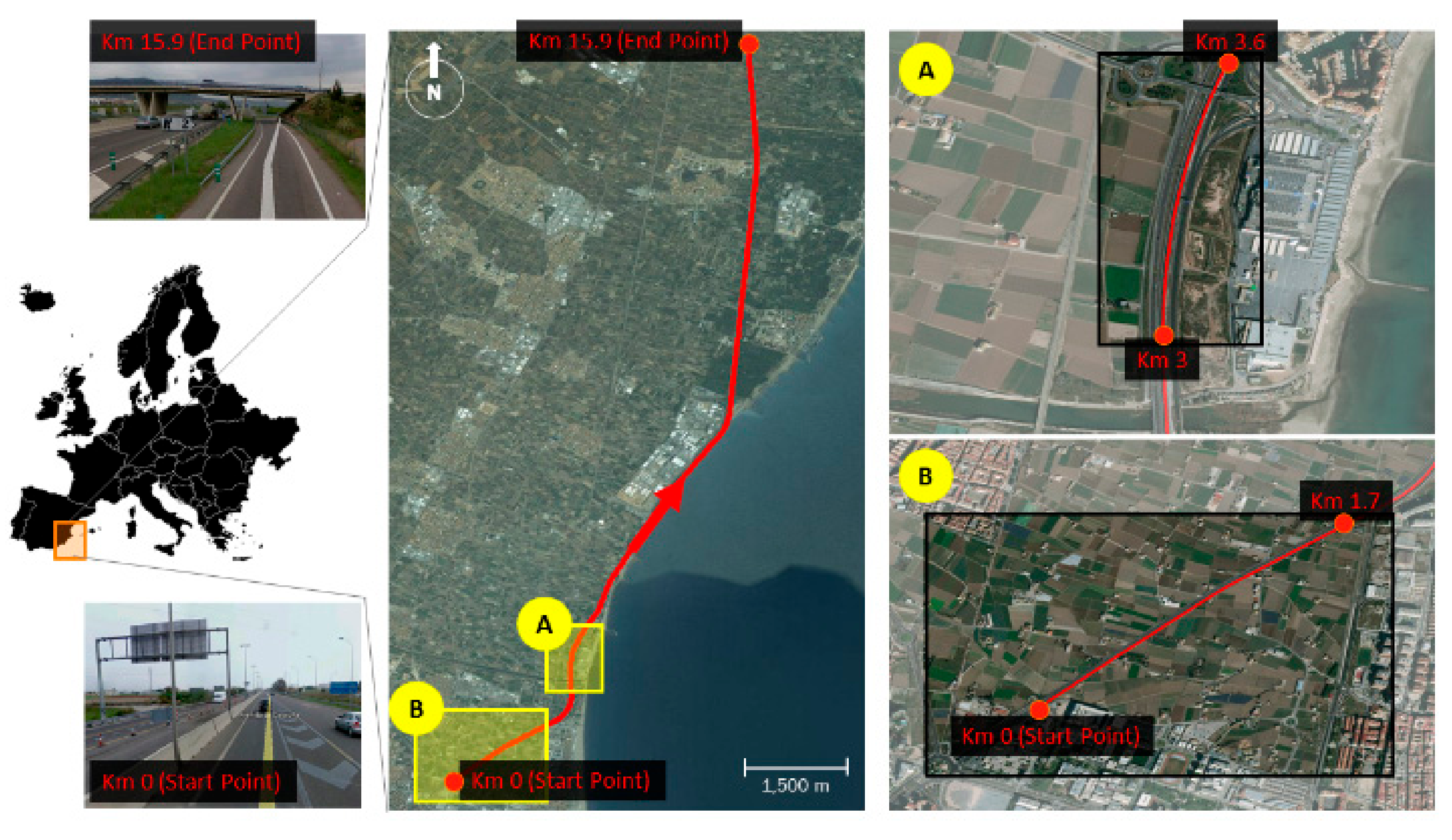
3. Data and Study Area

The data presented here were obtained in PROLOGUE, one of the most ambitious attempts to carry out a naturalistic driving trial at European level [43]. INTRAS (University Research Institute on Traffic and Road Safety) conducted the pilot study of PROLOGUE in Spain. This Spanish pilot trial was carried out in the surroundings of the city of Valencia, the third most populated city in Spain, during the months of June and July 2010. In short, five drivers participated for four days each. They drove a fully monitored vehicle, called Argos, for approximately two hours per day.
Around 80 parameters related to the driving performance of the different subjects were continuously recorded using different instruments and devices. Thus, the kinematic data related to speed, acceleration, and the braking force at any time were recorded. Furthermore, cameras also recorded both the interior and the surroundings of the vehicle, including, of course, the driving activities such as how often the driver interacted with any device. All these parameters were recorded at different temporal frequencies, depending on the technical specifications of each measuring device. The parameters related to kinematics were recorded at temporal frequencies of 10-2 s and 10-3 s. A more detailed description of the measuring devices used by Argos in the Spanish trial is shown in Valero-Mora et al. [44].
The data plotted in the following figures are uniquely related to the kinematic parameters in specific sections of the V-21 motorway, which links the city of Valencia and Puzol (Figure 1). This is a route of 15.9 km, which was traveled in both directions. This is the same route as the one considered in previous articles by the same authors.

4. Methodology and Results

Mapping of kinematic parameters is based on a working methodology different from what is commonly used to map events that are spatially fixed. These kinematic data permit the modeling of how one subject really drives under real world conditions. These data display the variations caused by the surrounding conditions at any time and/or place.
GIS systems provide three basic geometries or entities for mapping: points, (poly)lines, and polygons. All of them are used for mapping our data. However, this procedure is not straightforward and some preprocessing steps are required. For this purpose, a point array corresponding to the road section traveled is initially set up. GNSS and INS devices allow for the coordinates of each point to be obtained. Once a point array is set up over the road section, this can be easily defined in the software as a lineal entity.
The spatial distribution of points with data along the road path (actual point array) is irregular (Figure 2a) as it depends on the positioning and speed of the vehicle at any time. However, positioning data are not always available and consequently some strategies for estimating these coordinates must be implemented, such as the one presented in [27]. When that happens, we must draw a common road path, which coincides with the central axis of the road.
To represent these data and to perform some geoprocessing operations require that points must be regularly distributed along the road path. For this, we must define a theoretical point array along it (Figure 2b). The difference in the point distribution between both point arrays requires assigning values to each point from the actual scenario to the theoretical one. For this, we interpolate values from the actual point array into the regular one for which purpose we use the algorithm Inverse Distance Weighting, a two-dimensional interpolation function [45]. Due to the points are sequentially distributed along the same lineal entity, the value of each point in the theoretical point array may be computed as:
X A i = X B i + X B i 1 2
where A refers to the theoretical scenario and B to the actual one.
Once data values are assigned to the theoretical point array, geoprocessing operations can be carried out. We use two different attributes for mapping: geometries and colors. These attributes may be used in isolation or in combination. Magnitudes are represented by geometries. These attributes are polygonal entities projected onto one or both sides of the road path. These polygons allow shapes that emerge on the axis of the road to be defined. The distance between the axis and the external contour of this shape allows the magnitude of one certain kinematic parameter to be represented. In this way, some different parameters can be simultaneously plotted by overlapping several data layers (Figure 3a). With regard to the color attributes, tone changes depict variations in magnitude for any parameter (Figure 3b).
The aforementioned methodology is illustrated in Figure 4. This road section is located in the first part of the route (study area A in Figure 1). The length of this road path is about 600 m. This road section comprises a curve to the east and an uphill segment with a steep slope preceding the curve. Figure 4 depicts the speed of one of the drivers who participated in the trial. These maps show a continuous variability in speed as well as drastic fluctuations in very short distances. It could be due to some intermittent traffic jams that may have blocked the traffic at that time. However, the shape and slope of these fluctuations, in addition to their frequency, indicate that these were probably due to random malfunctions in some instruments, as described in [41].
Figure 4 proposes different strategies for mapping values of speed. In the first three subfigures (from 4.a to 4.c), speed values are represented by using a semi-buffer projected only onto the left side of the road path. Notice that the range scale is adapted to the zoom level selected by the user. In addition to geometries, color attributes help to obtain a clearer and smarter representation of speed values, although they do not offer any additional information. The first subfigure, Figure 4a, plots how the speed values vary by using only geometric attributes. In order to do that, we use a single-colored polygonal shape projected onto the left side of the road path. Notice that the color attribute is only used for aesthetic purposes, not providing any additional information. The magnitude of speed values is inferred in relation to the blue (60 km/h) and orange (120 km/h) contours, which are drawn over points with the same values (i.e., isolines). These speed values correspond to the minimum and maximum legal speeds on Spanish motorways, respectively.
The polygonal shapes plotted in Figure 4b were generated using the tool for multiple buffering. These lines run parallel to the route path. Each of the internal lines represents a difference in speed values of 10 km/h with regard to the previous one. In addition, a discrete palette with 12 single colors is attached to the geometries. Thus, the speed at any point of the road path may be inferred by observing both geometric and color attributes.
Geometries and color attributes are also combined in Figure 4c. Both attributes represent speed values, although in a different way than the previous figures. Here, color attributes are vertically displayed in relation to the road path. The color palette is the same as that which we used in the previous figure. However, in this case, some additional intermediate colors were generated from the degradation effect of the colors located at the extremes. This degradation effect is achieved with a representation based on raster format.
The next figure, Figure 4d, plots a polygonal single-colored shape. It was drawn using a buffer projected onto both sides of the road path. The aim of this map is to show an augmented vision of the speed values, based solely on geometries. Thus, the color attribute does not intend to provide any additional information. Finally, Figure 4e uses the contrary effect. In this figure, speed variations are solely based on color attributes, while geometries do not provide any additional information. These colors are vertically displayed in relation to the road path. The color palette is the same as that which we used in Figure 4c, which is based on raster format.

5. Benefits

GIS mapping of naturalistic driving data shows some advantages and great potentialities at two different levels of detail: (a) macro-, and (b) micro-scale. Among them, the most relevant are:
(a)
At a macro-level of detail,
  • The facilitation of a more general perspective of the driver performance allowing standard and non-standard (or anomalous) driving behavior to be derived.
  • The rapid detection of anomalous behavior, such as fast speed driving, abnormal speed changes, slow and/or wrong reactions to hazardous situations, etc.
  • The influence of road path on certain kinematic parameters, such as braking, acceleration, and deceleration actions.
  • The analysis of driving performance under certain conditions related with particular environments, traffic congestions, weather, etc.
  • The establishment of common driving patterns based on different factors, such as daytime, genre, socioeconomic status, etc.
  • The implementation of strategies for quality control of data, taking into account that misleading data may appear due to eventual malfunctions in some of the devices [28,29].
(b)
At a micro-level of detail,
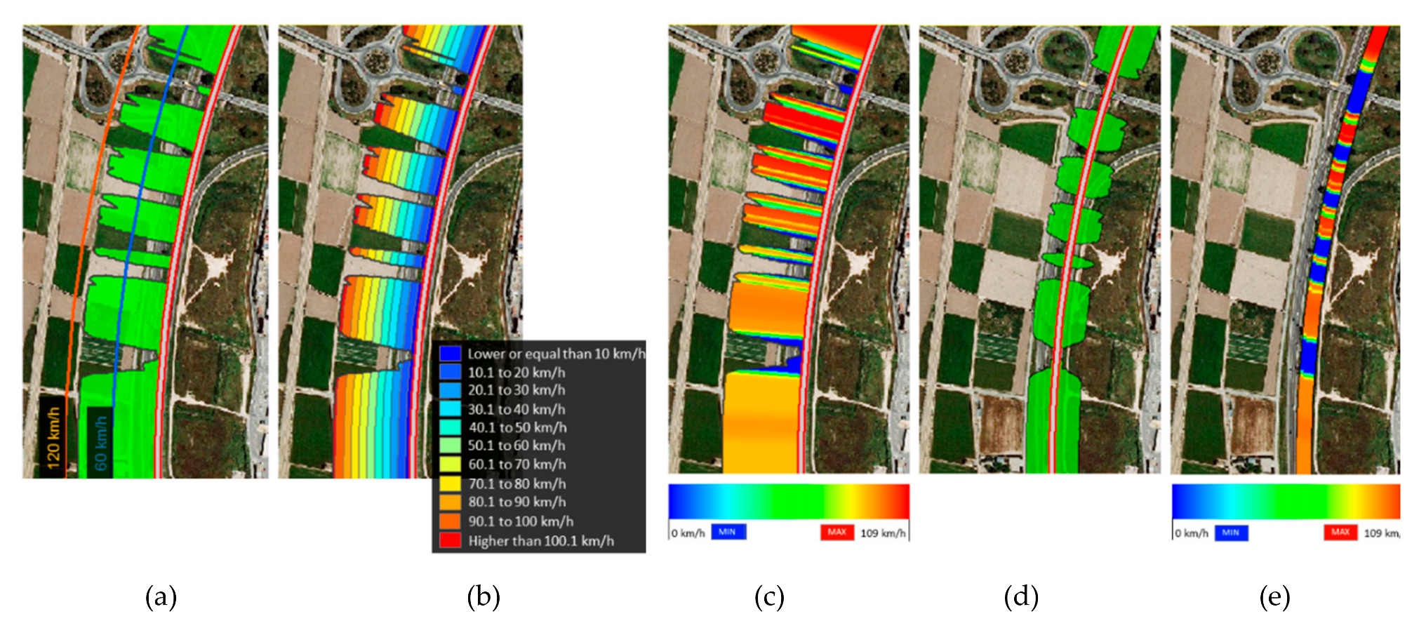
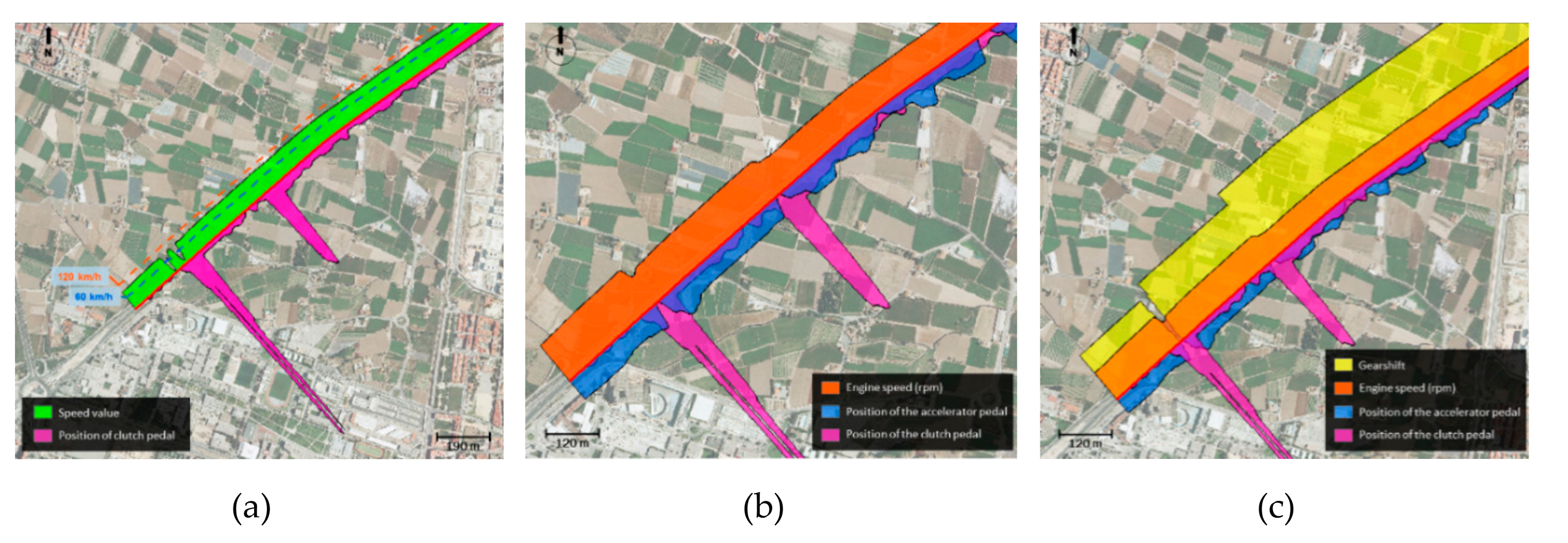
  • The achievement of a holistic vision of the driving performance for any subject. Thus, it is possible to analyze in detail how certain maneuvers (related to entry/exit in motorways, over-taking, and interactions between drivers and/or pedestrians) really happen. It is shown in Figure 5, where more data layers are sequentially included from left (two in Figure 5a) to right (four in Figure 5c).
  • The evaluation of the level of compliance with road signs and the degree of efficiency of awareness campaigns.
  • The detection of road sections that are potentially dangerous not only in terms of crashes, but also other incidents, such as near-crashes or anomalous behavior.

6. Discussion and Conclusions

Despite the evident spatial character of most traffic events, limited research has been conducted in road safety analysis to account for spatial correlation [46]. This reveals how GIS tools and geographical analysis still have very limited relevance to, and application on, road traffic. Regarding the studies that used GIS, but not necessarily reliant on naturalistic driving, these were focused on the representation of discrete events related to different traffic hotspots [47]. Aguero-Valverde and Jovanis [46] indicated the importance of including spatial correlation in road crash models at the segment level. They used a full Bayes hierarchical approach with conditional autoregressive effects for the spatial correlation terms. Jia, Khadka and Kim [48] presented a method using kernel density estimation with spatial clustering for explaining the macro distribution of traffic crashes using data related to points of interest. Zou et al. [49] implemented negative binomial models with K mixture components and varying weight parameters for crash hotspot identification. Fawcett et al. [50] proposed a Bayesian hierarchical model for predicting accident counts. All these studies apply different methodologies for identifying hotspots and for assessing how these are spatially distributed. Their results are confined to map the spatial distribution of discrete events (usually crashes) and/or highlight some vulnerable road sections by using simple entities, such as points and (poly)lines. Their results represent macroscopic traffic flows, the data of which were collected using traditional methodologies.
In turn, as this article tries to exploit the potentiality of naturalistic driving data, its goal and methodology is slightly different from the ones in these previous studies. For this, some strategies for mapping naturalistic driving were shown. The figures presented depict different kinematic (no discrete) parameters which allow the actual driving behavior be inferred at a micro-level of analysis.
Naturalistic driving has some common limitations with Big Data. In fact, the capacity for collecting data is much greater than our ability to process and analyze these data. This leads to an imbalance between the data we can collect, and the knowledge that we can gain from these data. For this reason, new software tools, research focus, and work methodologies are increasingly demanded for the purposes of expanding our capacity to exploit these data that are currently available.
Data from naturalistic driving trials present a great potential for assessing driving behavior in real traffic environments. Ideally, these studies require the integration of multidisciplinary work teams, which can apply different work methodologies and/or software tools. One of the biggest advantages of GIS systems is that they allow for these data to be visualized, analyzed, and geoprocessed in a smarter way than with other tools. This allows for a more comprehensive analysis of data by adding more information (data layers) and adjusting the spatial scale (zoom view). Thus, the conclusions are more trustworthy.
As yet, most software tools used in naturalistic driving present important restrictions, such as unfriendly user interfaces, limited processing capacity, and scarcely intuitive displays, among others. GIS tools allow most of these drawbacks to be overcome. These can handle and analyze relatively huge datasets, such as the one resulting from naturalistic driving trials. Indeed, they incorporate toolboxes for managing large volumes of data by aggregating millions of records into simple entities, such multipoint tool for LiDAR point clouds [51]. This avoids the need for final datasets to be thinned or limited to some specific road sections and/or events. In addition, geoprocessing tools implemented in GIS allow for managing and adjusting datasets to the concrete requirements at any time.
The very nature of the naturalistic driving method requires carrying out a greater data collection both in quantitative (more indicators) and qualitative terms (at higher temporal frequencies). However, it is often excessive for most research purposes, which complicates the successive tasks of the handling, managing, processing and analysis of the data. Therefore, we recommend introducing a preliminary phase in any study to give careful consideration to the right balance between the research aims and how the vehicle should be instrumented [22].
GIS mapping allows for a bigger picture of the driving performance and the whole scenario to be obtained. Thus, it is possible to evaluate not only how (and how much) a specific parameter varies in a road section, but also its location. Spatial context is one of the factors that can explain, at least partially, how drivers behave in some road sections. This is, again, a clear advantage of naturalistic driving data when considering an additional dimension (the spatial factor) that is usually determinant for the purposes of understanding the data.
The resulting maps can clearly represent the data, which simplifies and facilitates the subsequent phases related to the analysis and interpretation of these data. In addition, GIS systems provide a simple and friendly interface, which can be easily managed by users with a basic level of expertise in mapping. This approach enables experts from different fields of knowledge to be brought together in multidisciplinary work teams, which encourages the development of creative solutions for dealing with the multi-faceted problem that is road safety [19].
This study is a further step towards understanding our driving behavior better. In the case of naturalistic driving, GIS mapping presents great advantages in applications for quality control of data, for extracting driving patterns, and for detecting events, among others. Future studies should focus both on these research topics, and also on strategies about how to achieve a more efficient exploitation of naturalistic driving data.

Author Contributions

Conceptualization, J.B.-B. and P.M.V.-M.; Methodology, J.B.-B.; Validation, J.B.-B., P.M.V.-M., J.L.B.-V. and F.-A.V.-G.; Writing-Original Draft Preparation, J.B.-B.; Writing-Review & Editing, J.B.-B., P.M.V.-M., J.L.B.-V. and F.-A.V.-G.; Visualization, J.B.-B.; Supervision, J.B.-B., P.M.V.-M., J.L.B.-V. and F.-A.V.-G.; Project Administration, J.B.-B. and P.M.V.-M.; Funding Acquisition, J.B.-B., P.M.V.-M., J.L.B.-V. and F.-A.V.-G..

Funding

This research received no external funding.

Acknowledgments

The authors want to thank to the University Research Institute on Traffic and Road Safety (INTRAS) for providing the data we use in this study.

Conflicts of Interest

The authors declare no conflict of interest.

References

  1. Dulebenets, M.A. A comprehensive multi-objective optimization model for the vessel scheduling problem in liner shipping. Int. J. Prod. Econ. 2018, 196, 293–318. [Google Scholar] [CrossRef]
  2. Wagenaar, J.; Kroon, L.; Fragkos, I. Rolling stock rescheduling in passenger railway transportation using dead-heading trips and adjusted passenger demand. Transp. N.a. B Methodol. 2017, 101, 140–161. [Google Scholar] [CrossRef]
  3. Liu, L.; Chen, R.-C. A novel passenger flow prediction model using deep learning methods. Transp. N.a. C Emerg. Technol. 2017, 84, 74–91. [Google Scholar] [CrossRef]
  4. Jalalian, M.; Gholami, S.; Ramezanian, R. Analyzing the trade-off between CO2 emissions and passenger service level in the airline industry: Mathematical modeling and constructive heuristic. J. Clean. Prod. 2019, 206, 251–266. [Google Scholar] [CrossRef]
  5. Lindsey, C.R.; Vehoef, E. Traffic congestion and congestion pricing. In Handbook of Transport Systems and Traffic Control (Handbooks in Transport, Volume 3); Button, K.J., Hensher, D.A., Eds.; Emerald Group Publishing Limited: Bingley, UK, 2001; Volume 3, pp. 77–105. ISBN 978-0-08-043595-4. [Google Scholar]
  6. Lin, E.T.; Lan, L.W. Accounting for accidents in the measurement of transport inefficiency: A case of Taiwanese bus transit. Int. J. Sustain. Dev. 2009, 8, 365–385. [Google Scholar] [CrossRef]
  7. Balsa-Barreiro, J.; Ambuhl, L.; Menendez, M.; Pentland, A. ’Sandy’. Mapping time-varying accessibility and territorial cohesion with time-distorted maps. IEEE N.a. 2019, 7, 41702–41714. [Google Scholar] [CrossRef]
  8. Raffin, N.; Seegmuller, T. The cost of pollution on longevity, welfare and economic stability. Environ. Resour. Econ. 2017, 68, 683–704. [Google Scholar] [CrossRef]
  9. Forns, J.; Davdand, P.; Foraster, M.; Rivas, I.; Esnaola, M.; Garcia-Esteban, R.; Suades-Gonzalez, E.; Cirach, M.; Grellier, J.; Guxens, M.; et al. Traffic-related air pollution, noise at school, and behavioral problems in Barcelona schoolchildren: A cross-sectional study. Environ. Health Persp. 2016, 124, 529–535. [Google Scholar] [CrossRef] [PubMed]
  10. Dobbs, R.; Remes, J.; Manyka, J.; Roxburgh, C.; Smith, S.; Schaer, F. Urban World: Cities and the Rise of the Consuming Class, McKinsey Global Institute. 2012. Available online: https://www.mckinsey.com/global-themes/urbanization/urban-world-cities-and-the-rise-of-the-consuming-class (accessed on 14 March 2019).
  11. Buchanan, C. Traffic in Towns. A Study of the Long Term Problems of Traffic in Urban Areas, 1st ed.; Routledge: London, UK, 2015; ISBN 978-1138775992. [Google Scholar]
  12. Zheng, X. Determinants of agglomeration economies and diseconomies: Empirical evidence from Tokyo. Soc.-Econ. Plan. Sci. 2001, 35, 131–144. [Google Scholar] [CrossRef]
  13. Higano, Y.; Shibusawa, H. Agglomeration diseconomies of traffic congestion and agglomeration economies of interaction in the information-oriented city. J. Regional Sci. 1999, 39, 21–49. [Google Scholar] [CrossRef]
  14. Büscher, M.; Coulton, P.; Efstratiou, C.; Gellersen, H.; Hemment, D.; Mehmood, R.; Sangiorgi, D. Intelligent mobility systems: some socio-technical challenges and opportunities. In Proceedings of the 1st International Conference on Communications Infrastructure. Systems and Applications in Europe, London, UK, 11–13 August 2009; pp. 140–152. [Google Scholar]
  15. Schlingensiepen, J.; Mehmood, R.; Nemtanu, F.; Niculescu, M. Increasing sustainability of road transport in European cities and metropolitan areas by facilitating autonomic road transport systems (ARTS). In Proceedings of the 5th International Conference Sustainable Automotive Technologies, Ingolstadt, Germany, 25–27 September 2013; pp. 201–210. [Google Scholar]
  16. Evans, L. Traffic Safety; Science Service Society: Bloomfield Hills, MI, USA, 2004; Available online: http://www.scienceservingsociety.com/ts/rvs/AJPM.pdf (accessed on 14 March 2019).
  17. World Health Organization (WHO). Global Status Report on Road Safety; Department of Violence and Injury Prevention and Disability: Genève, Switzerland, 2010; Available online: https://www.who.int/violence_injury_prevention/road_safety_status/2018/en (accessed on 14 March 2019).
  18. Australian Road Research Board (ARRB). Guide to Road Safety Part 6: Road Safety Audit. 2009. Available online: https://www.onlinepublications.austroads.com.au/items/AGRS06-09 (accessed on 14 March 2019).
  19. NurFazzillah, M.N.; Mahmud, A.R.; Ahmad, N. Value-adding Safety Audit with GIS. Geospatial World. 2011. Available online: https://www.geospatialworld.net/article/value-adding-road-safety-audit-with-gis (accessed on 14 March 2019).
  20. Backer-Grøndahl, A.; Phillips, R.; Sagberg, F.; Touliou, K.; Gatscha, M. Topics and Applications of Previous and Current Naturalistic Driving Studies; Promoting Real Life Observations for Gaining Understanding of Road Behaviour in Europe, PROLOGUE (Deliverable D1.1); Institute of Transport Economics (TØI): Oslo, Norway, 2009; Available online: https://prologue.kfv.at/fileadmin/content/Dokumente/PROLOGUE_D1.1.pdf (accessed on 14 March 2019).
  21. McLaughlin, S.B.; Hankey, J.M.; Dingus, T.A. A method for evaluating avoidance systems using naturalistic driving data. Accident Anal. Prev. 2008, 40, 8–16. [Google Scholar] [CrossRef]
  22. Valero-Mora, P.M.; Tontsch, A.; Welsh, R. Is naturalistic driving research possible with highly instrumented cars? Lessons learnt in three research centres. Accident Anal. Prev. 2013, 58, 187–194. [Google Scholar] [CrossRef]
  23. Amediku, D. Application of GIS to Road Safety Auditing as an Option to Road Accident Management. Master Thesis, Kwame Nkrumah University, Kumasi, Ghana, 2000. [Google Scholar]
  24. Backer-Grøndahl, A.; Lotan, T.; van Schagen, I. Summary and Integration of a Series of Naturalistic Driving Field Trials; Promoting Real Life Observations for Gaining Understanding of Road Behaviour in Europe, PROLOGUE (Deliverable D3.7); Institute of Transport Economics (TØI): Oslo, Norway, 2011; Available online: https://prologue.kfv.at/fileadmin/content/Dokumente/PROLOGUE_D3.7.pdf (accessed on 14 March 2019).
  25. Pilgerstorfer, M.; Runda, K.; Brandstätter, C.; Christoph, M.; Hakkert, S.; Ishaq, R.; Toledo, T.; Gatscha, M. Small Scale Naturalistic Driving Pilot; DaCoTa. Deliverable D6.3; Kuratorium für Verkehrssicherheit (KfV): Vienna, Austria, 2011; Available online:http://www.dacota-project.eu/Deliverables/DaCoTA_D6%203_Report%20on%20Small%20scale%20ND%20pilot%20Final_20120625.pdf (accessed on 14 March 2019).
  26. Balsa-Barreiro, J.; Pareja, I.; Tontsch, A.; Sánchez, M. Preprocessing of Data for Recovery of Positioning Data in Naturalistic Driving Trial. In Proceedings of the 3rd European Conference on Human Centred Design for Intelligent Transport Systems, Valencia, Spain, 14–15 June 2012; pp. 235–245. [Google Scholar]
  27. Balsa-Barreiro, J.; Valero-Mora, P.M.; Pareja, I.; Sánchez, M. Georeferencing naturalistic driving data using a novel method based on vehicle speed. IET Intell. Transp. Sy. 2013, 7, 190–197. [Google Scholar] [CrossRef]
  28. Balsa-Barreiro, J.; Valero-Mora, P.M.; Pareja, I.; Sánchez, M. Quality Control Procedure for Naturalistic Driving Data Using Geographic Information Systems. In Proceedings of the 4th European Conference on Human Centred Design for Intelligent Transport Systems, Vienna, Austria, 20 June 2014. [Google Scholar]
  29. Balsa-Barreiro, J.; Valero-Mora, P.M.; Pareja, I.; Sánchez, M. Proposal of GIS methodology for quality control procedures (QC) of data obtained in naturalistic driving studies. IET Intell. Transp. Sy. 2015, 9, 673–682. [Google Scholar] [CrossRef]
  30. Klauer, S.G.; Dingus, T.A.; Neale, V.L.; Sudweeks, J.D.; Ramsey, D.J. The Impact of Driver Inattention on Nearcrash/Crash Risk: An Analysis using the 100-car Naturalistic Driving Study Data; Virginia Tech Transportation Institute: Blacksburg, WV, USA, 2006. Available online:https://vtechworks.lib.vt.edu/bitstream/handle/10919/55090/DriverInattention.pdf (accessed on 14 March 2019).
  31. Dingus, T.A.; Klauer, S.G.; Neale, V.L.; Petersen, A.; Lee, S.E.; Sudweeks, J.D.; Perez, M.A.; Gupta, S.; Bucher, C.; Jermeland, J.; et al. The 100-car Naturalistic Driving Study, Phase II: Results of the 100-car Field Experiment; National Highway Traffic Safety Administration: Washington DC, USA, 2006; Available online: https://trid.trb.org/view/783477 (accessed on 14 March 2019).
  32. Stutts, J.; Feaganes, J.; Reinfurt, D. Driver’s exposure to distractions in their natural driving environment. Accident Anal. Prev. 2005, 37, 1093–1101. [Google Scholar] [CrossRef]
  33. Christoph, M.; van Nes, N.; Pauwelussen, J.; Mansvelders, R.; van der Horst, R.; Hoedemaeker, M. In-vehicle and Site-based Observations of Vehicles and Cyclists; a Small-scale ND Field Trial in the Netherlands; Promoting Real Life Observations for Gaining Understanding of Road Behaviour in Europe, PROLOGUE (Deliverable D3.4); Nederlandse Organisatie voor Toegepast Natuurwetenschap-pelijk Onderzoek (TNO): Soesterberg, The Netherlands, 2010; Available online: https://prologue.kfv.at/fileadmin/content/Dokumente/PROLOGUE_D3.4.pdf (accessed on 14 March 2019).
  34. Wang, B.; Hallmark, S.; Savolainen, P.; Dong, J. Crashes and near-crashes on horizontal curves along rural two-lane highways: Analysis of naturalistic driving data. J. Safety Res. 2017, 6, 163–169. [Google Scholar] [CrossRef]
  35. Xiong, H.; Bao, S.; Sayer, J.; Kato, K. Examination of drivers’ cell phone use behavior at intersections by using naturalistic driving data. J. Safety Res. 2015, 54, 89–93. [Google Scholar] [CrossRef]
  36. Lassarre, S.; Dozza, M.; Jamson, S.; Lai, F.; Saad, F.; Vadeby, A.; Trent, V.; Brower, R.; Carsten, O.; Disilvestro, A.; et al. FESTA Support Action. Data Analysis and Modelling. Field Operational Test Support Action (Deliverable D2.4). 2008. Available online: https://dspace.lboro.ac.uk/dspace-jspui/bitstream/2134/5705/1/AR2604%20FESTA%20D2%204%20Data%20analysis%20and%20modeling.pdf (accessed on 14 March 2019).
  37. Gatscha, M.; Brandstätter, C.; Pripfl, J. Video-based Feedback for Learner and Novice Drivers: A Small-scale ND Field Trial in Austria; Promoting Real Life Observations for Gaining Understanding of Road Behaviour in Europe, PROLOGUE (Deliverable D3.3); Test and Training International (TTI): Teesdorf bei Baden, Austria, 2010; Available online: https://prologue.kfv.at/fileadmin/content/Dokumente/PROLOGUE_D3.3.pdf (accessed on 14 March 2019).
  38. Jovanis, P.; Aguero-Valverde, J.; Wu, K.; Shankar, V. Naturalistic driving event data analysis: omitted variable bias and multilevel modeling approaches. Transp. Res. Record. 2011, 2236, 49–57. [Google Scholar] [CrossRef]
  39. Val, C.; Küfen, J. Data Processing Framework Supporting Large Scale Driving Data Analysis. MATLAB Virtual Conference. 2013. Available online: https://www.mathworks.com/videos/data-processing-framework-supporting-large-scale-driving-data-analysis-92591.html (accessed on 14 March 2019).
  40. Dozza, M. SAFER100Car: A Toolkit to Analyze Data from the 100 Car Naturalistic Driving Study. In Proceedings of the 2nd International Symposium on Naturalistic Driving Research, Blacksburg, VW, USA, 31 August–2 September 2010. [Google Scholar]
  41. Balsa-Barreiro, J. Application of GNSS and GIS Systems to Transport Infrastructures. Study Focusing on Naturalistic Driving. PhD dissertation, Dept. of Civil Engineering, University of A Coruna (Spain) and Politecnico di Torino (Italy), 2015. Ph.D. Dissertation, Dept. of Civil Engineering, University of A Coruna, Coruna, Spain, Politecnico di Torino, Italy, 2015. [Google Scholar]
  42. Gordon, T.; Green, P.; Kostyniuk, L. A Multivariate Analysis of Crash and Naturalistic Event Data in Relation to Highway Factors Using the GIS Framework. In Proceedings of the 4th SHRP-2 Safety Research Symposium, Washington DC, USA, 23–24 July 2009; Available online: http://onlinepubs.trb.org/onlinepubs/shrp2/07SYM-KosGreen.pdf (accessed on 14 March 2019).
  43. Van Schagen, I.; Welsh, R.; Backer-Grøndahl, A.; Sagberg, F.; Tsippy, L.; Hoedemae, M.; Morris, A. Towards a Large-scale European Naturalistic Driving Study: Main Findings of PROLOGUE; Promoting Real Life Observations for Gaining Understanding of Road Behaviour in Europe, PROLOGUE (Deliverable D4.2); Institute for Road Safety Research (SWOV): Leidschendam, The Netherlands, 2011; Available online: https://dspace.lboro.ac.uk/dspace-jspui/bitstream/2134/9341/5/D4.2.pdf (accessed on 14 March 2019).
  44. Valero-Mora, P.M.; Tontsch, A.; Pareja, I.; Sánchez, M. Using a Highly Instrumented Car for Naturalistic Driving Research: A Small-scale Study in Spain; Promoting Real Life Observations for Gaining Understanding of Road Behaviour in Europe, PROLOGUE (Deliverable D3.5); Instituto de Tráfico y Seguridad Vial (INTRAS): Valencia, Spain, 2010; Available online: https://prologue.kfv.at/fileadmin/content/Dokumente/PROLOGUE_D3.5.pdf (accessed on 14 March 2019).
  45. Shepard, D. A Two-dimensional Interpolation Function for Irregularly-spaced Data. In Proceedings of the 23rd ACM National Conference, New York, NY, USA, 27–29 August 1968; pp. 517–524. [Google Scholar]
  46. Aguero-Valverde, J.; Jovanis, P.P. Analysis of road crash frequency with spatial models. Transport Res. Rec. 2008, 2061, 55–63. [Google Scholar] [CrossRef]
  47. Mitra, S. Enhancing Road Traffic Safety: A GIS Based Methodology to Identify Potential Areas of Improvement. Ph.D. Dissertation, Depart. of Civil and Environmental Engineering, University, San Luis Obispo, CA, USA, 2008. [Google Scholar]
  48. Jia, R.; Khadkab, A.; Kim, I. Traffic crash analysis with point-of-interest spatial clustering. Accident Anal. Prev. 2018, 121, 223–230. [Google Scholar] [CrossRef]
  49. Zou, Y.; Ash, J.E.; Park, B.; Lord, D.; Wu, L. Empirical Bayes estimates of finite mixture of negative binomial regression models and its application to highway safety. J. Appl. Stat. 2018, 45, 1652–1669. [Google Scholar] [CrossRef]
  50. Fawcett, L.; Thorpe, N.; Matthews, J.; Kremer, K. A novel Bayesian hierarchical model for road safety hotspot prediction. Accident Anal. Prev. 2017, 99, 262–271. [Google Scholar] [CrossRef] [PubMed]
  51. Balsa-Barreiro, J.; Lerma, J.L. A new methodology to estimate the discrete-return point density on airborne LiDAR surveys. Int. J. Remote Sens. 2014, 35, 1496–1510. [Google Scholar] [CrossRef]
Figure 1. Route between the city of Valencia (start point) and Puzol (end point). The data plotted in the following figures correspond to the road sections shown in rectangles A and B.
Ijgi 08 00226 g001
Figure 2. Point array distributed along the road path: (a) Actual, and (b) theoretical distribution.
Ijgi 08 00226 g002
Figure 3. Methodology for the representation of kinematic driving parameters using attributes based on (a) geometries and (b) colors.
Ijgi 08 00226 g003
Figure 4. Speed of one driver in study area A. Different mapping results using geometric and color attributes.
Ijgi 08 00226 g004
Figure 5. Kinematic driving parameters related to the performance of one subject in study area B. Different mapping results using geometric and color attributes.
Ijgi 08 00226 g005

