Article

Reliability Analysis of LandScan Gridded Population Data. The Case Study of Poland

Faculty of Civil Engineering and Geodesy, Military University of Technology, 00-908 Warsaw, Poland
*
Author to whom correspondence should be addressed.
ISPRS Int. J. Geo-Inf. 2019, 8(5), 222; https://doi.org/10.3390/ijgi8050222
Submission received: 22 March 2019 / Revised: 23 April 2019 / Accepted: 4 May 2019 / Published: 8 May 2019

Abstract

:
The issue of population dataset reliability is of particular importance when it comes to broadening the understanding of spatial structure, pattern and configuration of humans’ geographical location. The aim of the paper was to estimate the reliability of LandScan based on the official Polish Population Grid. The adopted methodology was based on the change detection approach, spatial pattern and continuity analysis, as well as statistical analysis at the grid-cell level. Our results show that the LandScan data can estimate the Polish population very well. The number of grid cells with equal people counts in both datasets amounts to 10.5%. The most and highly reliable data cover 72% of the country territory, while less reliable ones cover only 4.3%. The LandScan algorithm tends to underestimate people counts, with a total value of 79,735 people (0.21%). The highest underestimation was noticed in densely populated areas as well as in the transition areas between urban and rural, while overestimation was observed in moderately populated regions, along main roads and in city centres. The underestimation results mainly from the spatial pattern and size of Polish rural settlements, namely a big number of shadowed single households dispersed over agricultural areas and in the vicinity of forests. An excessive assessment of the number of people may be a consequence of the well-known blooming effect.

1. Introduction

A better understanding of many phenomena and processes related to the Earth’s surface requires information on the locations and characteristics of humans. The problem of reliable population distribution is being increasingly raised in the Earth and life sciences, particularly urban geography, health geography, crime geography, risk management, natural hazard exposure, ecology, climate change and many others. Detailed, timely and reliable information on the spatial distribution of people is important for local and regional communities, and therefore, it constitutes to be an important element of land administration systems [1].
The official providers of population data are national census agencies. They give the most reliable and the most complete information on population distribution related to pre-defined units, the size of which depends on the country and population density. Despite the undoubted advantages, statistical population data also have a number of drawbacks widely discussed in literature. As stated by [2], the main disadvantages are: long intervals between censuses and changes in borders of dissemination units, which make the data outdated and incomparable. Moreover, in many geographical regions, particularly those of irregular and dispersed population distribution, statistical data aggregated to administrative units’ gives an unrealistic view of the location of humans. This problem has been noticed by scientists as early as the beginning of the 20th century. The Russian cartographer Tian-Shansky coined the term ‘dasymetric mapping’ and elaborated the first dasymetric population density map of European Russia, scale 1:420,000, published in the 1920s [3].
Recent years have witnessed a significant increase in publicly available spatial datasets showing global or regional population distribution in a regular grid. The benefits of using grid cells as an alternative for administrative units comprise: undemanding data comparison over space and time, straightforward integration with other geographical data and easy data aggregation. Gridded population of the world (GPW) was the first global, spatially consistent, and commonly available dataset that adopted Tobler’s smooth pycnophylactic (mass-preserving) interpolation algorithm for transformation of census population to a grid [4,5,6,7]. The GPW was the core source data for the Global Rural-Urban Mapping (GRUMP) project. GRUMP delivered more reliable human distribution data thanks to the use of complementary geographical data (e.g., footprint of urban centres, settlement point location) and satellite data, especially NOAA’s night-time lights images [4,8]. LandScan is the third world-wide population database that characterises an ambient, averaged over 24 hours, humans’ geographical distribution in 30 arc-second resolution [9]. People counts, as integer values, are attributed to a 30 sec. grid in WGS 84 (Word Geodetic System) datum. The constantly revised multi-variable dasymetric ‘smart’ interpolation algorithm integrates a recently updated number of auxiliary geographical data, mainly derived from high-resolution satellite imagery [10,11]. Since the year 2000, LandScan has been updated annually. However, regularly revised methods and supplementary data are not conducive to version comparison. In 2013, GPW, GRUMP and LandScan initiated the broader studies on people distribution for low-income countries of Africa, Asia and South America resulting in the common project WoldPop [12]. The WorldPop 100 m gridded population datasets depict a reliable representation of population distributions based on census data supplemented with a variety of geographical data including social media [13] or cell phones [14,15].
In 2010, the Joint Research Centre (JRC), the European Commission's science and knowledge service, initiated the concept of the Global Human Settlement Layer (GHSL). GHSL delivers data on people’s presence in the world in the form of thematic maps (layers); namely, built up, population density and settlement maps. The disaggregation approach relies on built-up data as a threshold to limit and improve the distribution of people [16]. A brief description of global population datasets is presented in Table 1.
Literature presents many metrics for comparative evaluation of raster population distribution. Most of them are based on pixel level and detailed official population datasets delivered by census agencies and perceived as ground truth data. The simplest ones measure the differences between two datasets, more advanced, geo-referenced metrics originate from geostatistics, meteorology or signal processing [17]. Moreover, errors of the population estimation are generally measured by RMSE, MAE, MAPE, omission and commission [12,18,19,20,21,22]. However, the ability to validate the global raster population data is still very limited because no independent sources exist that could serve this purpose. Validation of global gridded population surfaces hitherto has based on crosschecking with population totals reported by the UN (for GPW and GRUMP) or by the national official sources for LandScan and GHS-POP. The results show that, for most of the countries, the differences in population counts are insignificant [15,18,22,23,24,25,26]. Other studies, e.g., [13,21], also highlight overall good correspondence of the total population, especially in low income countries. Nevertheless, in some regions, like the coastal zone, these differences are significant [20]. Moreover, [20] found that large differences in population counts are dominant in those countries where the estimation of population spatial distribution was based on outdated and course input data. Some researchers [18,20,21,22,23,24] also noticed that the simple areal weighting algorithm used to generate the GPW and GRUMP sometimes leads to considerable estimation errors, while the approach based on advanced ‘smart’ methods and a huge set of ancillary data (such as LandScan, WordPop) gives a better assessment of population.
The objective of this paper was to estimate the comprehensive, cell-based reliability of LandScan data using the set of metrics, setting up the criteria of reliable data, and to portray spatial distribution of reliability classes in a user-friendly and efficient way. The selection of LandScan was supported by the following reasons. Primarily, the literature review shows that LandScan, with a more advanced dasymetric algorithm and a broad scope of satellite derived detailed ancillary data provides the best estimates of people counts [11,17,18,23,24].
Moreover, LandScan dataset is of common interest of researchers from all over the world and diversified scientific disciplines e.g., remote sensing, geosciences, environmental, urban and engineering studies, meteorology, health geography, demography and geophysics [11,17,20,21,22,23,24]. The number of articles indexed inWeb of Science (WoS) and Scopus databases on LandScan usability and potential applications equals 66 (from 2009 to 2018), and is several times higher than other global population datasets (see Table 1). LandScan is the only global population dataset that has been updated annually since 2000. Therefore, it can be used to analyse the trends in demography and geographical distribution of population according to urbanisation, suburbanisation or urban sprawl. Moreover, the preliminary analysis conducted by [27], based on the comparison of total population of Poland and global gridded population datasets, found that LandScan corresponds to Polish census data (available in 1 km grid) better than GRUMPv1 and GPWv4. The Pearson coefficient of correlation between census people counts and the population estimated by LandScan, GRUMPv1, and GPWv4 equals 0.72, 0.52 and 0.49, respectively.
The presented analysis is a step forward to gridded population data usability and fit for purpose studies, not only for Poland, but also for any region with an irregular and scattered settlement network, where dispersed population distribution is observed (e.g., Eastern and Southern European Countries). The novelty and main scientific contribution of this study relay on establishing the method of estimated population data reliability evaluation based on simple statistical and GIS measures.
The analysis facilitates understanding the relations between the two information outputs, which differ in the population disaggregation approaches. Moreover, the issue of reliability of population datasets is of particular importance when it comes to broadening the understanding of spatial structure and the pattern or configuration of the geographical location of humans. The main objectives of the study are in line with the questions regarding:
-
What is the relatedness of LandScan and Polish Population Grid data?
-
What is the spatial pattern of highly over- and underestimated areas?
-
What is the relation between reliability classes and the types of built-up area and the district status?
The method can be easily duplicated to assess the reliability (or uncertainty) of any gridded population datasets at the cell level. The results can be used to identify regions that are particularly difficult to estimate people counts in grid format, and hence, to further improve dasymetric modelling techniques.
The next section (Section 2) provides a description of the area, methods and data used; the results are presented and discussed in Section 3 and Section 4. The paper ends with a brief concluding section.

2. Area, Materials and Methods

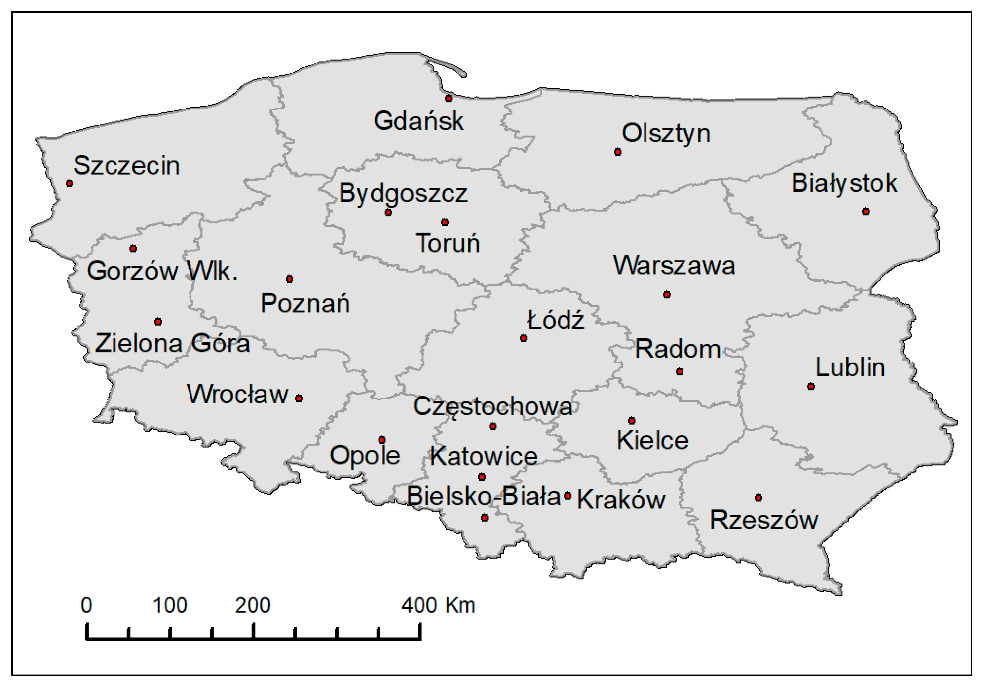
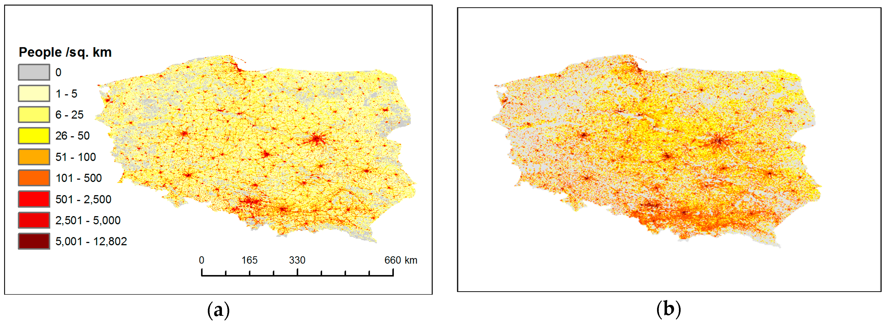
2.1. Overview of Polish Population

Poland is inhabited by 38,492,223 people [28], and is the ninth most populous country in Europe and 33rd in the word, constituting 5.4% of the European and 0.5% of the word population. Total population is almost stagnant, with the population growth lower than 0.08% [28]. 61.5% of the country population lives in urban areas, namely 930 cities with an average population density of 1105 people per 1 km2. Population density in rural areas is over 22 times lower, and equals 50 people per 1 km². The country average is 123 people/km². The capital city, Warsaw, counts more than 1.764 million inhabitants, with 3,412 population density, and is the biggest Polish city. The current population of Poland was shaped by political and economic changes, especially economic recession, development of agriculture and industry, and the most of the country border changes as a result of many wars, particularly, the First and the Second Word Wars. The settlement network is dominated by big cities located in the central and southern part of the country, and relatively small numbers of cities in the peripheral regions (Figure 1). According to [29], the population distribution in Polish cities is characterised by the exponential model, with a noticeable decline in population density at distances of 3.0–3.5 km from the centre. Moreover, the depopulation of city centres is rather rarely observed, and takes place in just a few Polish cities. This led [30] to the conclusion that current urbanisation in Poland differs significantly from that of highly-developed countries, and it is not justified to say that the Polish population distribution has a de-urbanization trend.

2.2. The Source Data

The release of LandScan 2012 (the 14th version of LandScan) Global Population Database was used in this study. The main improvements of this release include updating country census data. Temporal consistency was achieved by normalising census count on July 2012 using national population estimates provided by the CIA World Factbook. Moreover, urban built-up areas and thousands of smaller villages and populated places were refined or added based on high-resolution imagery. Finally, the spatial precision and values of the population distribution were substantially improved. The LandScan 2012 Global Population Database at 30 arc-seconds (1 km or finer) was delivered by ORNL in raster ESRI Grid format on July 15, 2013 (see Figure 2a).
Polish Population Grid (PPG) represents residential population of the year 2011 (Figure 2b). It is the official dataset created by the Central Statistical Office (CSO). The number of inhabitants attributed to each square kilometre cell is assigned on the basis of the Population and Housing Census 2011 by addresses and dwelling geolocation [31]. Thus, the data represent the number of people staying at home at night, i.e., the population of place of residence at night time. This dataset is further perceived as reference data. PPG is tailored to European standards by way of data processing and storage, as well as preserving statistical confidentiality. Hence, the smallest number of people assigned to one grid cell equals 3, which is the nationwide average number of people in one household. The dataset was made within the frame of GEOSTAT11, the project established by Eurostat, the European Statistical Office. The data are available via geostatistical portal [32] in ESRI shp format. Figure 2 shows the spatial distribution of people according to both analysed gridded population data, LandScan (left) and PPG (right), by choropleth map. Each cell is coloured one of nine possible shades to show the places from uninhabited (grey), thinly (yellow), moderately (red), till very dense (brown) populated areas in Poland. The colour scheme follows the rules of census population cartography [33].
Built-up areas, stored in the General Geographic Database (BDOO), were used to analyse the relationship between the reliability of LS data and the built-up areas (namely: multi and single family residential, industrial, commercial, and other). BDOO is the official georeferenced set of data at the level of detail corresponding to a 1:250,000 scale map. The boundaries of second level (district) administration division were obtained from the state Register of Boundaries (PRG), which is the official dataset and constitutes the main reference frame for statistical data [34].

2.3. Methods Used

The reliability of spatial data refers to the degree to which they portray the reality in a sufficiently complete and error-free way to be convincing for their purpose and context. Reliability means that any errors found within a tolerable range (threshold) are not significant and do not disturb conclusions, findings or recommendation based on the data. It could be expressed as a parameter associated with the data that characterises the dispersion of the values that could reasonably be attributed to the measured ones.
LandScan (LS) reliability analysis methodology comprises three different approaches:
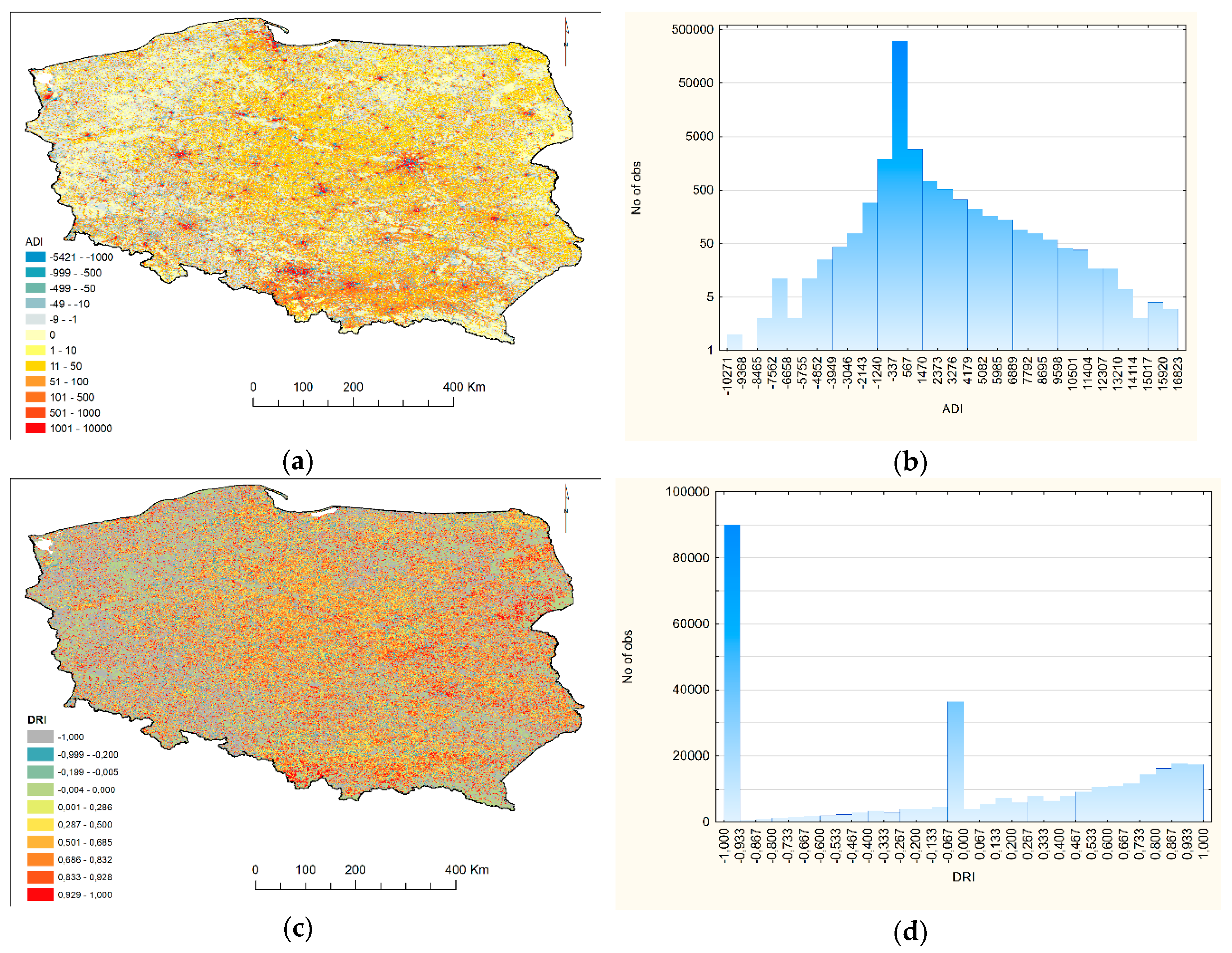
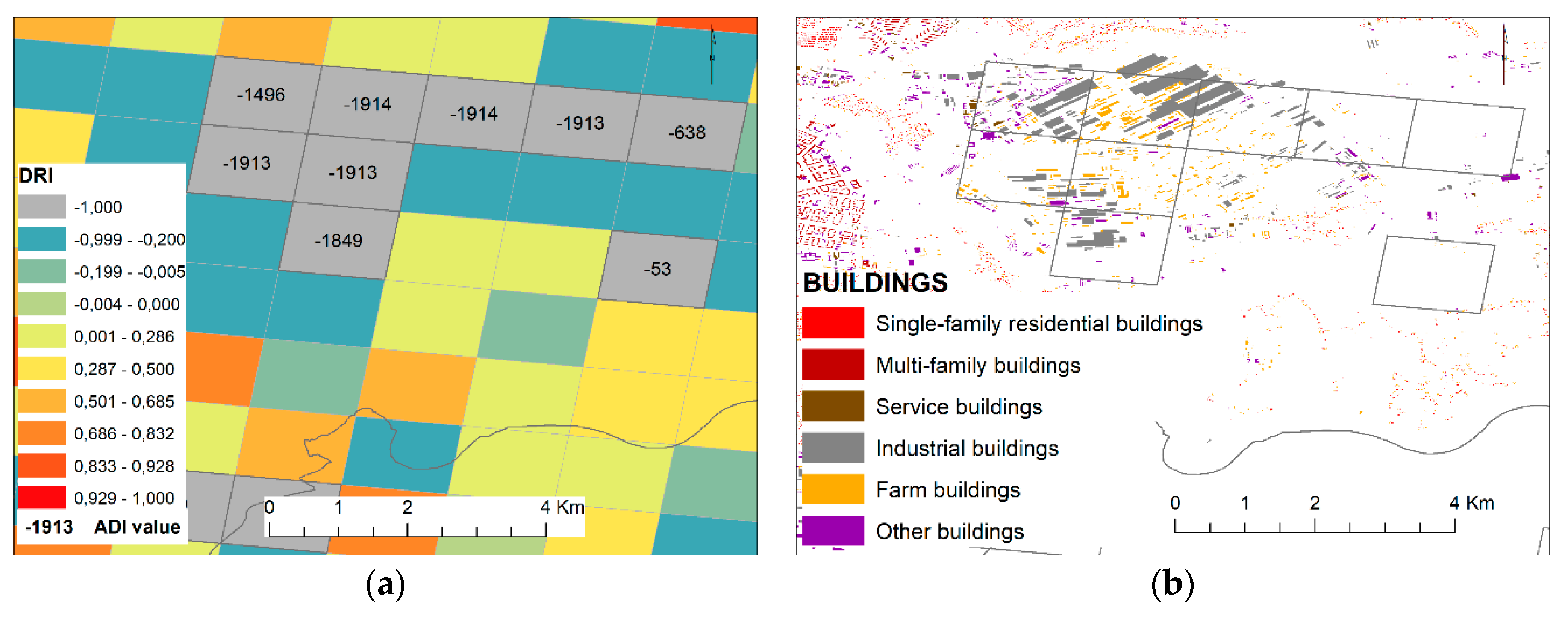
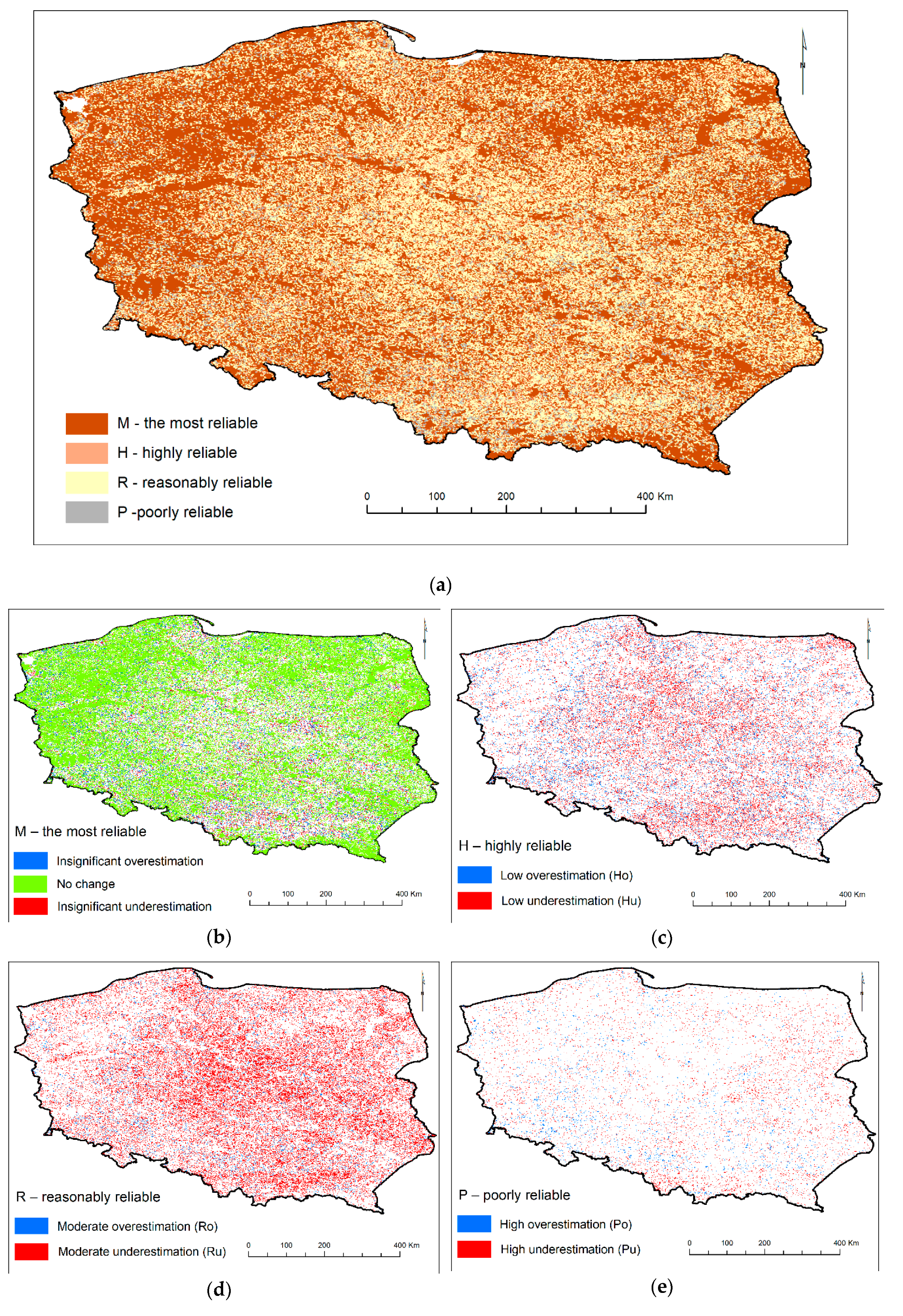
  • Change in the detection approach to obtain discrepancies at the grid cell level measured by two disparity indexes. The values of these indices constituted the basis for determining the LS reliability classes.
  • GIS and spatial incremental statistics approach to analyse the spatial pattern of the population reliability classes expressed by the Spatial Contiguity Index (SCI) index and Average Nearest Neighbour (ANN) ratio.
  • Statistical approach to investigate the concentration of reliability classes presented by statistical measure of concentration and dispersion, relations between reliability classes and built-up areas and the type of administrative units.
The quantification of LS reliability bases on the general assumption that the Polish Population Grid (PPG) is a reference dataset. The disparity indices, i.e., the absolute disparity index (ADI) and the deviation rate index (DRI), are computed on cross-comparison analysis of all corresponding grid cells in considered datasets, namely PPG and LS. They indicate how much the LS values deviate from the PPG. The absolute disparity index (ADI), similar to absolute estimation error (AEE), measures the total difference in people counts in each i- spatial location (grid cell), and is expressed as (Equation (1)):
A D I i = P P G i L S i ,
The ADI takes values from the range < LSmax; PPGmax>. A value lower than 0 means data overestimation, while a value greater than 0 means an underestimation of LS data.
The deviation rate index (DRI) is defined as (Equation (2)):
D R I i =   P P G i   L S i P P G i + L S i ,
DRIi is derived from the assumption that the deviation rate is the difference between the LSi population estimated data and the average of PPGi and LSi expressed as P P G i + L S 1 2 . The DRI values are normalised between −1 and +1. Values near zero indicate small differences, while values close to −1 and 1 show great discrepancy in population counts. Values lower than zero depict overestimation, and higher than zeroshow underestimation of PPG population counts in the corresponding area, represented as a grid cell. DRI takes value 1 for PPG = 0 and LS ≠ 0 and -1 for PPG ≠ 0 and LS = 0.
The LandScan data reliability quantification is based on the disparity indices and a general assumption that the threshold of population counts is 9 (triple average number of people in the household). This means that −9 ≤ ADI ≤ 9 depicts highly reliable data. The median mean absolute deviation (MAD) was used to establish the reliability classes. For PPG = 0 and LS ≠ 0 or PPG ≠ 0 and LS = 0 DRI takes the value of 1 or -1, respectively, without a possibility to assess the rate of over- or underestimation of population by LS data. That is why the ADI index has to be used to determine the level of reliability. Finally, the four LS reliability classes were distinguished, namely: the most reliable, highly reliable, reasonably reliable and poorly reliable, as presented in the Table 2.
The spatial pattern of reliability classes was assessed by the Average Nearest Neighbour (ANN) ratio analysis and the Spatial Contiguity Index (SCI). The ANN statistics was calculated as the observed average distance between spatial objects divided by the expected average distance. The expected average distance is based on a hypothetical random distribution with the same number of features covering the same total area. The significance of the results was tested by p-value. An ANN ratio value lower than 1 means that the pattern of each class exhibits clustering. Otherwise, the trend is toward dispersion [35].
The Spatial Contiguity Index (SCI) uses a statistic called polygon neighbours, defined by Lai et al. [36] as a measure of polygons contiguity. The index is calculated for four adjacent grid neighbours, according to the formula given by Calka [37] (Equation (3)):
S C I = 1 n   s   4 m n
where: n—the number of reliability classes; m—the number of grid cells in a given reliability class; s—the number of neighbours in the same class. The SCI takes vales from 0 to 1, with 0 for a highly dispersed reliability class (low proximity), and 1 for a highly concentrated class (high proximity).
Finally, the map depicting varying degrees of reliability associated with each LandScan grid cell was proposed in a form of a choropleth map, according to the rules established by [38].

3. Results

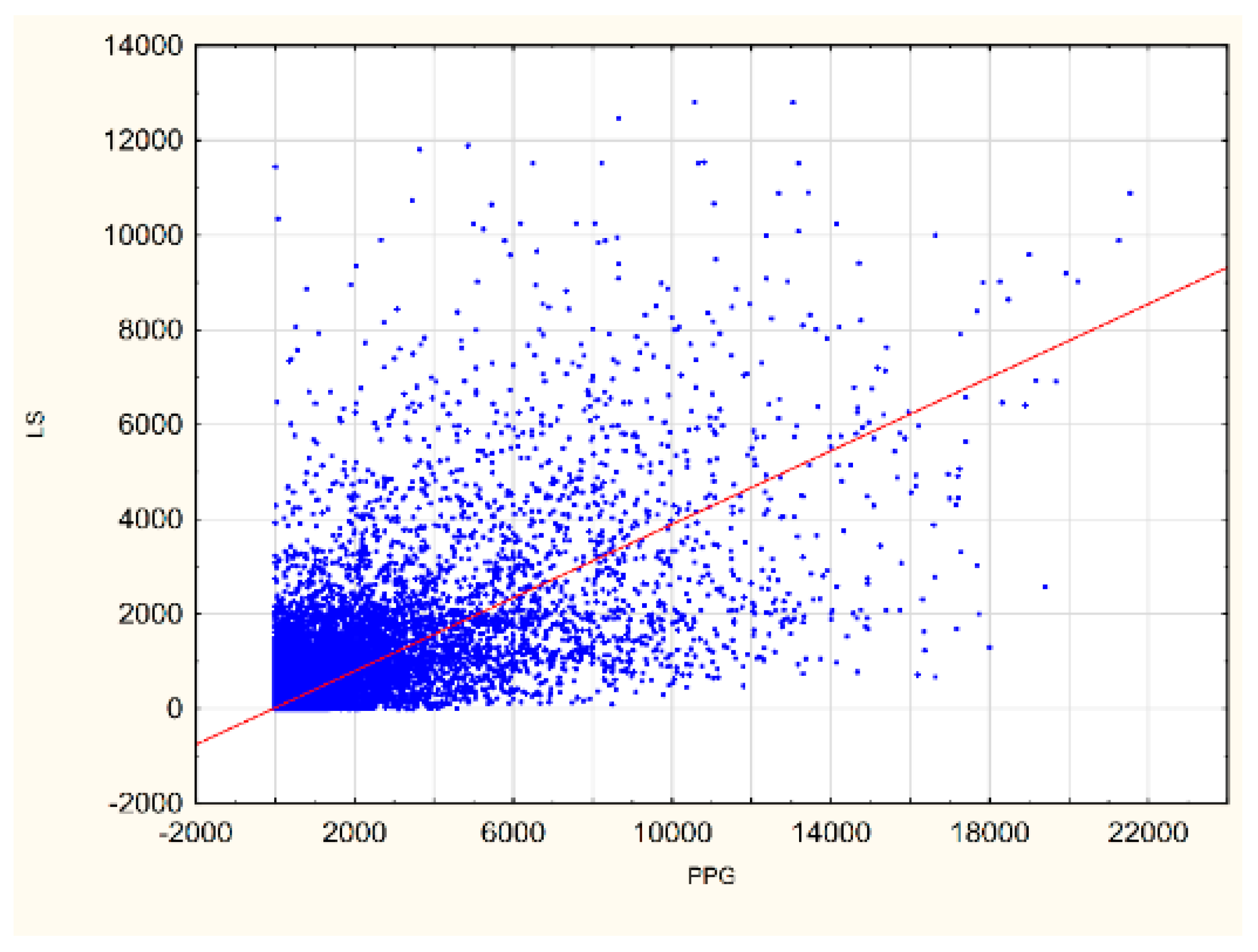
3.1. Relatedness of LandScan and Polish Population Grid Data

Gridded population data varies sharply across the country territory, with the minimum value of 0 for uninhabited areas, to the largest number of people per 1 km2, which equals to 21,531 in PPG and 12,802 in LS. The measures of central tendency (mean, median, mode), as well as the measures of dispersion such as variance, standard deviation and interquartile range (Table 3) emphasise the high variability of population distribution, and show the general population underestimation of LS data. The total underestimation counts 79,735 people, which corresponds to 0.21% of Polish population. However, for sparsely populated areas, LS tends to overestimate the people counts (Table 3—lower quartile (Q1) values).
The coefficient of the simple linear regression between PPG and LS equals to 0.74 and the coefficient of determination R2 takes the value of 0.55 (with p < 0.0000, and standard error of estimate 231.43). However, the observed spread of data (Figure 3) does not entitled to draw any conclusions regarding the matching between LS and PPG data based only on R2 and slope of the regression line.
The number of grid cells with equal population counts in both datasets (ADI = 0 and DRI = 0) amounts to 32,946 (10.5%), overestimated data constitutes of 40.4%, while underestimated constituted of 49.1 % of all cells. For 35.7% of the cells, the differences in people counts did not increase by over nine persons. These data are perceived as the most reliable. The overestimation greater than 5,000 people occurred in 56 grid cells, 4999–1000 people—in 1,274 cells (0.41%), and 999–500 people—in 20,625 grid cells (6.6%) (see Figure 4a–b). The highest overestimation of 10,271 people was found in Warsaw, while the largest underestimation took a value of 12,802. Counts larger than 100 people were noted in 69,039 (22.1%) cells, while larger than 5,000 were noted in 1,339 (0.43%). The DRI values from the range of <−0.999; −0.945> enhance the overestimation; however, they comprised only a few cells (320 cells, 0.1%). In general, the highest overestimation was observed in city centres (Figure 4c). The DRI equals -1 for at least 90,000 cells (28.65%), where PPG = 0 and LS ≠ 0 (see Figure 4d).
Analysis of these grid cells shows that for 25%, the overestimation does not exceed 2 persons; for 75%, it does not exceed 8 persons; and for 90% it does not exceed 18 people. Moreover, for 80% the ADI takes values from the range of <−9; −1>, which means it has the highest reliability. The DRI values close to 1 point to high underestimation, with 8,676 cells (2.8%) of values in the range of <0.999; −0.945>. Investigation of these cells indicates that for 10% grids the overestimation does not exceed 3 persons, i.e., the Polish average number of people in one household, and the middle 50% (interquartile range) amounts to 26 people. The underestimation is clearly visible in densely populated areas, mainly cities, along main roads and in the sparsely populated transition areas between urban and rural, while overestimation is present in moderately populated and almost unpopulated regions to balance the totals.

3.1.1. Reliability of LandScan Data

The most reliable data comprise 56.9% of all grid cells (Figure 5b, Table 4), out of which for 46.2% the LandScan estimation equals the values assigned by Polish reference statistical population data (PPG). About 5% of cells that belong to this class tend to have an insignificant under- or overestimation of no greater than 9 persons. This confirms the preliminary statement concerning high reliability of LandScan data, and its relatedness with PPG of nearly 57%. Highly reliable data constitute 15.1%, of which 10.7% tend to low underestimation, and 4.4% overestimate the official people counts a little (Figure 5c). Reasonably reliable data cover 23.7%, with 21.3 % of moderate underestimation (Figure 5d). Low quality, poorly reliable data constitute just 4.3%, of which 3.1% are highly underestimated (Figure 5e).
The most reliable data are dispersed over the whole country and form irregular continuous clusters (SCI = 0.33) of different sizes: the biggest ones are found in forests and the smallest ones in urban areas. Highly and reasonably reliable classes contain weakly clustered data (Figure 5c,d) with the ANN ratio values close to 1 (Table 5). These clusters are formed by several grid cells that share borders, which is highlighted by low SCI values: 0.07 and 0.11, respectively. Highly uncertain data are also clustered (Figure 5e), but the cells share borders with a few adjacent elements (SCI = 0.05).

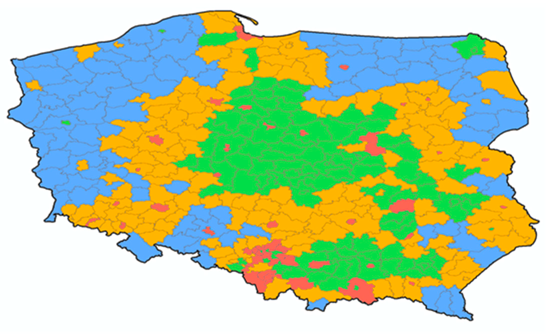
3.1.2. Relatedness with Built-Up Areas and District Status

Built-up areas cover 41.7% of the country territory, of which 91.3% constitute residential built-up (88.5% single-family and 2.8% multifamily housing). The estimation of people counts in single-family housing areas varies significantly. The most reliable data account for 31.1%, highly reliable – 24.0%. Reasonably reliable data cover 37.4% of single-family housing areas and tend to moderate underestimation (34.7), while poorly reliable data comprise only 7.4% of single-family housing and indicate high underestimation (6.7%) of people counts. Population estimation in multifamily housing areas is almost infallible for 30.7% and very good for 34.1%. Reasonably reliable data cover 30.0% with evident moderate underestimation (27.4%), while poorly estimated population data constitute 5.0%, 3.8% of which are highly underestimated. In the industrial zones, the most reliable data constitute 35.6%, while in commercial as much as 32.7% of areas. The worst estimation (poor reliability) covers 5.3% of commercial zones and 10.3% of industrial areas. To balance the totals, the moderate and high overestimation of the population (Ro, Po) occurs primarily in industrial and commercial zones (about 30.3%), single-family housing (3.1%), and multifamily housing (3.8%) areas.
Moreover, the LandScan algorithm overestimates people counts in agricultural areas, where settlement network is spatially dispersed. Figure 6 illustrates the overestimation in the fringe part of Krakow, the metropolitan centre located in southern Poland, with a 770 thousand inhabitants and average population density of 2354 person per sq. kilometre. The grey cells indicate DRI values equal to 1, what means unpopulated areas according to Polish Census Data (PPG), the numbers point out the value of overestimation, namely the ADI value. The overestimation indicated assigning too many people to industrial warehouse and farm buildings by LS dasymetric algorithm (Figure 6b). Furthermore, the correlation analysis indicates lack of dependence between the LS reliability classes and population density in districts. The Pearson coefficient (PCC) indicates a moderate positive relationship between population density and the percentage share of reasonably reliable LS data. For the remaining reliability classes this dependence is negative and weak (see Table 6).
The minimal share of the most reliable data in districts, which are the second level of administration division in Poland, amounts to 20.9%, while the maximum reaches 84.2%, with the mean of 52.2%. The inadequately estimated population data (Poor LS class) range from zero to 21.9%, with the mean value of 5.1% and standard deviation of 3.1% (Table 6). The classification of districts by k-means algorithm, according to the share of LandScan reliability classes distinguishes four regions (Figure 7). The red one comprises heavily urbanised and densely populated cities, which are district centres. This group contains as much as 58% of the global range of the most reliable data (see Table 6), and takes the highest value of poorly reliable data that fall outside the upper quartile (73.7%). The region marked in blue covers sparsely populated ‘land’ districts, with a significant percentage of forest areas and agricultural land. The LS estimates people counts there very well; the share of the most reliable data is the highest with the value of 58.85%, while poorly reliable data are in the range of global lower quartile (27.88%).
The green region reflects districts with the highest value of reasonably reliable data (68.14%), as well as a relatively low share of the most and poorly reliable data: 37.3 and 39.6%, respectively, that fall in the lower global quartile. The LS data tends to moderate underestimation. The golden group of districts is not spatially continuous; it comprises 134 districts with varied population density (min. 24, max. 2898, mean 174 people per 1 km²). Share of the most and poorly reliable data equal to 31.5 and 48.5%, respectively. The LandScan data tend there to moderate or low overestimation.

4. Discussion

Any dasymetric modelling is subjective, which has been broadly discussed in literature [1,3,11]. The subjectivity and, consequently, the uncertainty arises from the disaggregation algorithm and the imperfection of ancillary data [3,39]. The importance of uncertainty in dasymetric modelling has not yet been sufficiently recognized. LandScan uses a big set of data and allocates empirical weighing factors to data layers as well as sub-categories within these data [4,5,6,10,11]. Hence, the results of people allocation to grid-cells are very good. However, the variability of the real word, its physiographic, cultural and socioeconomic diversity, cause enormous difficulties in adjusting the model for individual grid-cell level.
The adopted methodology of LandScan reliability analysis is simple and based on well-known statistical and GIS measures of dispersion. Comparing this methodology with others presented in the literature, we noted both similarities and differences in the approaches to assessing the accuracy of estimated gridded population datasets. The difference indexes of people counts in two analysed datasets, which were adopted in this study, resemble those described in other studies. The absolute disparity index (ADI) corresponds to absolute estimation error defined by Bai et al. [18], fractional area coverage described by Sabesan et al. [17], or omission rate used by Potere el al [40]. At the same time, the deviation rate index (DRI) definition is similar to the difference dataset index computed by Hall et al. [26] and difference rate implemented by Oyabu et al. [41]. Furthermore, similar to [17,25,26,41], we attributed accuracy to the grid cell, whereas [10,13,18,23,24] accuracy results are more vague and refer to administrative units.
Despite the relatively extensive research on global population data quality, only a few studies defined the levels of accuracy or uncertainty. For example, Bai et al. [18], based on relative estimation error (REE), established five categories of accuracy of gridded population datasets for China using thresholds of 25, 50 and 100% of REE. Nowak et al. [25] also classified uncertainties up to five degrees, adjusting class thresholds to natural breaks in the histogram of differences in population counts. Aubrecht et al. [42] showed the diversity of gridded population data for Austria in five ranges, but the final quality assessment was generalised to the district level. Our approach to defining the reliability classes of gridded population data, besides providing information of underestimated, overestimated or unchanged data (in five degrees), also provides information on the level of data significance, referred to by the names of reliability classes, as: most reliable, highly, reasonably and poorly reliable. This gives users a broader view of information value concerning the quality of population distribution in a given area.
Comparable to [17,18,26], reliability in our study reflects similarity to the census counts rather than an absolute ground truth. Furthermore, this reliability depends on the threshold of ADI and DRI indexes. Along with the increase in the ADI threshold, the number of grid cells recognized as ‘no change’, and thus belonging to the most reliable uncertainty class, increases. However, this upsurge is not significant and equals 15% for the very pessimistic assumption of PPG uncertainty in people counts amounts to 18 persons for each 1 km2. The increase of LS grid cell attributed to the most reliable class is balanced by a slight decrease in highly and reasonably reliable classes. It is worth noting that the number and spatial distribution of LS cells that are characterized by the most significant uncertainty in population estimation (those belonging to the poorly reliable class) basically did not change. The sensitivity analysis of ADI threshold impact on LandScan grid cell allocated to reliability classes (as per cent of total number of grid cells) is shown in Table 7.
The threshold of DRI is based on median absolute deviation (MAD) values, a robust measure of the variability of quantitative data, which is very insensitive to the presence of outliers. The threshold depends strongly on the stringency of the researcher's criteria, and according to Leys et al. [43] the median plus or minus 2.5 or even 2.0 times the MAD for outlier detection is recommended. In our study, the median of DRI takes the value of 0, with the maximum equal to 1, and the minimum equal to −1 (see Table 3). The MAD amounts to 0.633. Hence, the stringent MAD threshold cannot exceed 1.5 (i.e., 0.944).
The analysis assumes that Polish Populated Grid, elaborated by Central Statistical Office on the bases of full statistical survey, works as a ground truth data, which definitely influences the final results. The accuracy of census data and subsequently the ability to tie them to a specific location was previously discussed by [17,18,24,25]. As stated by [44], coverage, sampling and nonresponse are sources of error common to all statistical surveys. However, due to introducing some IT techniques (e.g., portable, hand-held terminals with the possibility of respondents’ geolocation) during the 2011 census in Poland these errors decreased significantly [45]. Moreover, the census data show where people are officially registered, and that could differ from where they really live. According to [29], this is mainly observed in big cities; for example, in Warsaw the actual population could be even 6–10% greater than official statistics say.
The Polish settlement network is dispersed and comprises more than 56.6 thousand small villages or other rural settlement units like hamlets or lodges. Tree-covered, dispersed along agricultural lands, single homesteads are almost impossible to detect on satellite images [4,17,46]. Moreover, insufficiently illuminated small settlements do not give the blooming effect on the night-time lights satellite scenes [8,11], and consequently provide rather to underestimation than overestimation. The highest population overestimation in the centres of the cities confirms the findings of [29,30] concerning depopulation of Polish big cities. Moreover, the VmapL2 used data from the years 2000–2002 as an ancillary source for Poland [47], i.e., it portrayed the reality 10 years earlier. This definitely resulted in omission of residential houses and even small settlements.
The overall accuracy assessment of LandScan data for Poland measured by RMSE equals to 467.90. Comparing the results with those achieved by [25], LandScan outperforms the GRUMP gridded population data in Poland. Similar findings were noticed by [26]. However, the observed differences in people counts assigned to a grid-cell in Sweden far outweigh those in Poland. The relatedness of LS, measured by R2, in Poland and Sweden is as far as 0.55 and 0.59, respectively. However, they are much lower than those received by [11] for Los Angeles county and Ellis county (CA, USA), which are 0.81 and 0.93, respectively.
However, this simple method, suited for cell-to-cell evaluation, is also appropriate for other units (e.g., administrative, towns, coastal zones). The comparison of two gridded population datasets shows in particular their similarity (or dissimilarity); hence, the method could be applied to assess the relatedness of analysed sets. Moreover, it can be quickly implemented to compare any gridded population datasets at the cell based level. The established reliability classes of LandScan can also act as classes of similarity (or relatedness) of analysed data sets. This is especially important when analysing any gridded population datasets, without the initial assumption that one of them is less uncertain.

5. Conclusions

One of the fundamental problems of spatial data users is the awareness of data reliability, particularly the information where people counts are under or overestimated. The lack of comprehensive approaches for reliable quantification of grid-based, high-resolution global population data limits their use in decision support and is perceived as the main drawback of those datasets. This paper takes a step towards formal reliability quantification by developing a set of tools to evaluate the utility of gridded population data, particularly LandScan.
The presented results show how well LandScan data correspond to population distribution derived from statistical census. Although LandScan algorithms are tailored to match the geographical nature and economic conditions of each country and region, the reliability of population distribution in Poland differs. For densely populated regions, LS underestimates the number of people, while for thinly populated ones it is rather overestimated, which reflects the settlement network, forest and agricultural regions location.
The most important conclusion of our research is the high reliability of LandScan data for Poland. The most reliable data amount to 56.9% and form irregular clusters, while highly reliable data cover 15.1% and are weakly clustered. Data of definitely insufficient quality cover only 4.2% with an evident trend to underestimation, especially in industrial and commercial zones of big cities.
The analysis of district type and the LS reliability shows that population counts in urban districts are characterised by both high percentage of very well and rather weak estimations. At the same time, in ‘landed’ districts, the LS reliability negatively corresponds with population density.
In the future, we will focus on eliminating the shortcomings of the developed methodology for assessing the relatedness of population datasets and providing more insights into the comparison between LS and PPG. In particular, we will examine how the population of small villages is estimated by LS, and analysing omission errors based on the official Polish gazetteer. Moreover, the proposed ADI and DRI indices as well as the thresholds will be used to assess reliability of other global population data, and for other countries.

Author Contributions

B.C. and E.B. conceptualised the study; B.C. performed all analysis; E.B. and B.C. analysed results, made conclusions and wrote the paper.

Funding

The research was carried out as part of the statutory work realized in years 2015–2018 at the Military University of Technology in Warsaw, Poland, Grant number PBS 933/2018.

Acknowledgments

This product was made utilizing the LandScan (2013)™ High Resolution global Population Data Set copyrighted by UT-Battelle, LLC, operator of Oak Ridge National Laboratory under Contract No. DE-AC05-00OR22725 with the United States Department of Energy. The United States Government has certain rights in this Data Set. Neither UT-Battelle, LLC nor the United States Department of Energy, nor any of their employees, makes any warranty, express or implied, or assumes any legal liability or responsibility for the accuracy, completeness, or usefulness of the dataset. LandScan data was purchased from the Oak Ridge National Laboratory for the United States Department of Defense in July 2013. The Polish Population Grid was obtained from the Central Statistical Office resources (http://geo.stat.gov.pl/atom_web-0.1.0/download/), BDOO and administrative units were derived from the Head Office of Geodesy and Cartography official web site (http://www.codgik.gov.pl/index.php/darmowe-dane).

Conflicts of Interest

The authors declare no conflict of interest. The funders had no role in the design of the study; in the collection, analyses, or interpretation of data; in the writing of the manuscript, or in the decision to publish the results.

References

  1. Pirowski, T.; Bartos, K. Detailed mapping of the distribution of a city population based on information from the national database on buildings. Geodetski Vestnik 2018, 62, 458–471. [Google Scholar] [CrossRef]
  2. Gregory, I.N.; Marti-Henneberg, J.; Tapiador, F.J. Modelling long-term pan-European population change from 1870 to 2000 by using geographical information systems. J. R. Stat. Soc. 2010, 173, 31–50. [Google Scholar] [CrossRef]
  3. Bielecka, E. A dasymetric density population map of Poland. In Proceedings of the ICC/ICA Conference in a Coruna, Barcelona, Spain, 9–16 July 2005. [Google Scholar]
  4. Balk, D.; Yetman, G. The Global Distribution of Population: Evaluating the Gains in Resolution Refinement; Center for International Earth Science Information Network (CIESIN), Columbia University: New York City, NY, USA, 2005; Available online: http://beta.sedac.ciesin.columbia.edu/gpw/docs/gpw3_documentation_final.pdf (accessed on 20 May 2018).
  5. Hay, S.I.; Noor, A.M.; Nelson, A.; Tatem, A.J. The accuracy of human population maps for public health application. Trop. Med. Int. Health 2005, 10, 1073–1086. [Google Scholar] [CrossRef] [PubMed]
  6. CESIN—Center for International Earth Science Information Network Columbia University. Gridded Population of the World, Version 4 (GPWv4): Data Quality Indicators, Beta Release; NASA Socioeconomic Data and Applications Center (SEDAC): Palisades, NY, USA, 2015. [Google Scholar] [CrossRef]
  7. Doxsey-Whitfield, E.; MacManus, K.; Adamo, S.B.; Pistolesi, L.; Squires, J.; Borkovska, O.; Baptista, S.R. Taking Advantage of the Improved Availability of Census Data: A First Look at the Gridded Population of the World, Version 4. Appl. Geogr. 2015, 1, 226–234. [Google Scholar] [CrossRef]
  8. Balk, D.L.; Deichmann, G.; Yetman, F.; Pozzi, S.; Hay, I.; Nelson, A. Determining Global Population Distribution: Methods, Applications and Data. Adv. Parasitol. 2006, 62, 119–156. [Google Scholar] [CrossRef]
  9. Dobson, J.; Bright, E.; Coleman, P.; Durfee, R.; Worley, B. A Global Population database for Estimating Populations at Risk. Photogramm. Eng. Remote Sens. 2000, 66, 849–857. [Google Scholar]
  10. Bhaduri, B.; Bright, E.; Coleman, P. Development of a high resolution population dynamics model. Paper Presented at Geocomputation, Ann Arbor, MI, USA, 1–3 August 2005; Available online: http://www.geocomputation.org/2005/Abstracts/Bhaduri.pdf (accessed on 20 May 2018).
  11. Bhaduri, B.; Bright, E.; Coleman, P.; Urban, M. LandScan USA: A high-resolution geospatial and temporal modeling approach for population distribution and dynamics. Geojournal 2007, 69, 103–117. [Google Scholar] [CrossRef]
  12. Calka, B.; Nowak Da Costa, J.; Bielecka, E. Fine scale population density data and its application in risk assessment. Geomat. Nat. Hazards Risk 2017, 8, 1440–1455. [Google Scholar] [CrossRef]
  13. Linard, C.; Kabaria, C.W.; Gilbert, M.; Tatem, A.J.; Gaughan, A.E.; Stevens, F.R.; Sorichetta, A.; Noor, A.M.; Snow, R.W. Modelling changing population distributions: An example of the Kenyan Coast, 1979–2009. Int. J. Digit. Earth 2017, 10, 1017–1029. [Google Scholar] [CrossRef]
  14. Deville, P.; Linard, C.; Martine, S.; Gilbert, M.; Stevens, F.R.; Gaughan, A.E.; Blondel, V.D.; Tatem, A.J. Dynamic population mapping using mobile phone data. Proc. Natl. Acad. Sci. USA 2014, 111, 15888–15893. [Google Scholar] [CrossRef] [PubMed]
  15. Liu, L.; Peng, Z.; Wu, H.; Jiao, H.; Yu, Y. Exploring Urban Spatial Feature with Dasymetric Mapping Based on Mobile Phone Data and LUR-2SFCAe Method. Sustainability 2018, 10, 2432. [Google Scholar] [CrossRef]
  16. Pesaresi, M.; Ehrlich, D.; Ferri, S.; Florczyk, A.J.; Freire, S.; Halkia, S.; Julea, A.M.; Kemper, T.; Soille, P.; Syrris, V. Operating Procedure for the Production of the Global Human Settlement Layer from Landsat Data of the Epochs 1975, 1990, 2000, and 2014; EUR 27741 EN; Publications Office of the European Union: Ispra, Italy, 2016. [Google Scholar] [CrossRef]
  17. Sabesan, A.; Abercrombie, K.; Ganguly, A.R.; Bhaduri, B.; Bright, E.A.; Coleman, P.R. Metrics for the comparative analysis of geospatial datasets with applications to high-resolution grid-based population data. GeoJournal 2007, 69, 81–91. [Google Scholar] [CrossRef]
  18. Bai, Z.; Wang, J.; Wang, M.; Gao, M.; Sun, J. Accuracy Assessment of Multi-Source Gridded Population Distribution Datasets in China. Sustainability 2018, 10, 1363. [Google Scholar] [CrossRef]
  19. Available online: http://www.fao.org/docrep/009/a0310e/A0310E07.htm (accessed on 10 September 2018).
  20. Merkens, J.-L.; Vafeidis, A.T. Using information on settlement patterns to improve the spatial distribution of population in coastal impact assessments. Sustainability 2018, 10, 3170. [Google Scholar] [CrossRef]
  21. Tatem, A.J.; Gaughan, A.E.; Stevens, F.R.; Patel, N.N.; Jia, P.; Pandey, A.; Linard, C. Quantifying the effects of using detailed spatial demographic data on health metrics: A systematic analysis for the AfriPop, AsiaPop, and AmeriPop projects. Lancet N. Am Ed. 2013, 381, S142. [Google Scholar] [CrossRef]
  22. Ma, Y.; Xu, W.; Zhao, X.; Li, Y. Modeling the Hourly Distribution of Population at a High Spatiotemporal Resolution Using Subway Smart Card Data: A Case Study in the Central Area of Beijing. ISPRS Int. J. Geo-Inf. 2017, 6, 128. [Google Scholar] [CrossRef]
  23. Mondal, P.; Tatem, A.J. Uncertainties in Measuring Populations Potentially Impacted by Sea Level Rise and Coastal Flooding. PLoS ONE 2012, 7, e48191. [Google Scholar] [CrossRef]
  24. Azar, D.; Engstrom, R.; Graesser, J.; Comenetz, J. Generation of fine-scale population layers using multi-resolution satellite imagery and geospatial data. Remote Sens. Environ. 2013, 130, 219–232. [Google Scholar] [CrossRef]
  25. Nowak Da Costa, J.; Bielecka, E.; Calka, B. Uncertainty quantification of the Global Rural-Urban Mapping Project over Polish census data. In Proceedings of the Environmental Engineering 10th International Conference, Vilnius, Lithuania, 27–28 April 2017. [Google Scholar] [CrossRef]
  26. Hall, O.; Stroh, E.; Paya, F. From census to grids: Comparing gridded population of the world with Swedish census records. Open Geogr. J. 2012, 5, 1–5. [Google Scholar] [CrossRef]
  27. Palczynska, P. Analysis of the Reliability of Global Population Density Data in Poland. Master’s Thesis, Military University of Technology, Warsaw, Poland, 2016. [Google Scholar]
  28. GUS. Ludność w Gminach Według Stanu w Dniu 31.12.2011 r.—Bilans Opracowany w Oparciu o Wyniki NSP 2011; Główny Urząd Statystyczny: Warsaw, Poland, 2012.
  29. Śleszynski, P. Delimitation of the Functional Urban Areas around Poland’s Voivodship Capital Cities. Przeglad Geograficzny 2013, 85, 173–197. [Google Scholar] [CrossRef]
  30. Korcelli, P.; Grochowski, M.; Kozubek, E.; Korcelli-Olejniczak, E.; Werner, P. Development of Urban-Rural Regions: From European to Local Perspective; Monografie IGiPZ PAN No 14; PAN IGiPZ: Warszawa, Poland, 2012. [Google Scholar]
  31. Migacz, T.M. Geostatistics Portal—A platform for statistical data geovisualization. Stat. J. IAOS 2015, 31, 463–470. [Google Scholar] [CrossRef]
  32. GUS. Available online: https://geo.stat.gov.pl/imap/?locale=en (accessed on 18 January 2019).
  33. Medynska-Gulij, B. Geovisualisation as a process of creating complementary visualisations: Static two-dimensional, surface three-dimensional, and interactive. Geod. Cartogr. 2017, 66, 89–104. [Google Scholar] [CrossRef]
  34. Bielecka, E.; Dukaczewski, D.; Janczar, E. Spatial Data Infrastructure in Poland—Lessons learnt from so far achievements. Geod. Cartogr. 2018, 67, 3–20. [Google Scholar] [CrossRef]
  35. Clark, P.J.; Evans, F.C. Distance to nearest neighbour as a measure of spatial relationships in populations. Ecology 1954, 35, 445–453. [Google Scholar] [CrossRef]
  36. Lai, P.; So, F.; Chan, K. Spatial Epidemiological Approaches in Disease Mapping and Analysis; Taylor & Francis Group: Boca Raton, USA, 2009. [Google Scholar]
  37. Calka, B. Comparing continuity and compactness of choropleth map classes. Geod. Cartogr. 2018, 67, 21–34. [Google Scholar] [CrossRef]
  38. Medyńska-Gulij, B. Map compiling, map reading and cartographic design in “Pragmatic pyramid of thematic mapping. Quaestiones Geographicae 2010, 29, 57–63. [Google Scholar] [CrossRef]
  39. Nagle, N.N.; Buttenfield, B.; Leyk, S.; Spleilman, S. Dasymetric modelling uncertainty. Ann. Assoc. Am. Geogr. 2014, 104, 80–95. [Google Scholar] [CrossRef]
  40. Potere, D.; Schneider, A.; Shlomo, A.; Civco, D.L. Mapping urban areas on a global scale: Which of the eight maps now available is more accurate? Int. J. Remote Sens. 2009, 30, 6531–6558. [Google Scholar] [CrossRef]
  41. Oyabu, Y.; Terada, M.; Yamaguchi, T.; Iwasawa, S.; Hagiwara, J.; Koizumi, D. Evaluation reliability of Mobile Spatial Statistics. NTT DOCOMOTO Tech. J. 2013, 14, 16–23. [Google Scholar]
  42. Aubrecht, C.; Yetman, G.; Balk, D.; Steinnocher, K. What is to be expected from broad-scale population data? Showcase accessibility model validation using high-resolution census information. In Proceedings of the 13th International Conference on Geographic Information Science, Guimarães, Portugal, 1–15 May 2010; pp. 1–7. [Google Scholar]
  43. Leys, C.; Ley, C.; Klein, O.; Bernard, P.; Licata, L. Detecting outliers: Do not use standard deviation around the mean, use absolute deviation around the median. J. Exp. Soc. Psychol. 2013, 49, 764–766. [Google Scholar] [CrossRef]
  44. Draugalis, J.R.; Plaza, C.M. Best Practices for Survey Research Reports Revisited: Implications of Target Population, Probability Sampling, and Response Rate. Am. J. Pharm. Educ. 2009, 73, 142. [Google Scholar] [CrossRef] [PubMed]
  45. Dygaszewicz, J. Geographical information systems in public statistics. Wiadomości Statystyczne 2011, 9, 19–31. [Google Scholar]
  46. Drzewiecki, W. Thorough statistical comparison of machine learning regression models and their ensembles for sub-pixel imperviousness and imperviousness change mapping. Geod. Cartogr. 2017, 66, 171–210. [Google Scholar] [CrossRef]
  47. Pokonieczny, K. Comparison of land passability maps created with use of different spatial data bases. Geografie 2018, 123, 317–352. [Google Scholar]
Figure 1. Poland. First level administration units (voivodships) and selected big cities.
Ijgi 08 00222 g001
Figure 2. Population distribution by LandScan (a) and Polish Population Grid (PPG) (b).
Ijgi 08 00222 g002
Figure 3. Scatterplot of PPG and LS.
Ijgi 08 00222 g003
Figure 4. Disparity indices: (a) ADI—absolute disparity index; (b) histogram of ADI values, the number of grid cells (vertical axis) is presented in logarithmic scale; (c) DRI—deviation rate index; (d) histogram of DRI values.
Ijgi 08 00222 g004
Figure 5. Spatial distribution of LS data reliability: (a) LS reliability classes; (b) the most reliable data; (c) highly reliable data; (d) reasonably reliable; (e) poorly reliable LS data.
Ijgi 08 00222 g005
Figure 6. Krakow: (a) overestimation of LandScan data presented by DGI index and ADI values for the most overestimated cells; (b) Building types delivered from National Topographic database.
Ijgi 08 00222 g006
Figure 7. Poland, districts classification according to share of LS reliability classes.
Ijgi 08 00222 g007
Table 1. Overview of global population datasets.
AbbreviationsGPWGRUMPLandScanGHSL
NameGridded Population of the WorldGlobal Rural-Urban Mapping ProjectLandScan (LS) Global PopulationGlobal Human Settlement Layer
Reference years of population estimation1990, 2000, 2005, 2010, prediction for 2015, 20201990, 1995, 20001998, from 2000 each year1975, 1990, 2000, 2014
Format spatial resolutionGrid/raster, ASCII
2.5 arc-minutes 30 arc-seconds for 2010
Grid/raster
30 arc-seconds
Grid
30 arc-seconds
TIF and OVR files 259 m, 1 km World Mollweide
Source and ancillary dataData from nation census agencies, water mask, coastlineGPW, urban mask, settlement points, NOAA’s night-time lights dataCensus data, roads, slope NIMA’s DTED, Global Land cover database, VMap, satellite imagery, night-time light NGDC, regional statisticsGPWv4, population censuses, Global, fine-scale satellite images, census data, volunteering geographic information sources
Method and algorithmDisaggregation of national census data, smooth pycnophylactic (mass-preserving) interpolationDisaggregation of national census data, smooth pycnophylactic (mass-preserving) interpolation Disaggregation sub-national census counts within administrative boundary, locally adoptive ‘smart’ interpolation algorithmSpatial data mining technologies
Data producerCIESIN & CIATCIESIN & IFPRI & CIAT & World BankORNLEuropean Commission Joint Research Centre (JRC)
Delivery policyCreative Commons Attribution 4.0 International LicenseCreative Commons Attribution 4.0 International LicenseAvailable for purchaseOpen and free data
Applications Demonstrate the spatial relationship of human populations and the environment (e.g., pollution, diseases, biodiversity) across the globeDelimitation of urban and rural areasTrends and demographic changes, risk assessment, strategic planning, and sustainable development, humanitarian aid and human well-being, people exposure to different types of hazardsCrisis management, demographic trends, monitoring urban growth and degree of urbanisation
Number of publication in WoS/Scopus databases 117/1312/1166/9329/40
1 Received on February 5, 2019.
Table 2. LandScan reliability classes.
Reliability ClassesRange of ADIRange of DRI
M—the most reliable−9 ≤ ADIi ≤ 9−0.5 MAD < DRIi < +0.5 MAD
H—highly reliable −1.0 MAD < DRIi ≤−0.5 MAD
or
0.5 MAD ≤ DRIi < +1.0 MAD
−1.0 MAD < ADIi ≤ −0.5 MAD
or
0.5 MAD ≤ ADIi < +1.0 MAD
DRI1 = 1 or DRI1 =−1
R—reasonably reliable------−1.5 MAD < DRIi ≤ −1.0 MAD
or
1.0 MAD ≤ DRIi < +1.5 MAD
−1.5 MAD< ADIi ≤ −1.0 MAD
or
1.0 MAD≤ ADIi < +1.5 MAD
DRI1 = 1 or DRI1 =−1
P—poorly reliable------−1.5 MAD ≤ DRIi
or
DRIi ≥ +1.5 MAD
−1.5 MAD ≤ ADIi
or
ADIi ≥ +1.5 MAD
DRI1 = 1 or DRI1 =−1
Table 3. Descriptive statistics of PPG, LS and disparity indexes.
Descriptive StatisticsPPGLSADIDRI
Min00−10,271−1
The first quartile (Q1)02−3.0−1
Median 12600
Mean123.16557.6−0.023
Mode000−1
The third quartile (Q3)651937.00.667
Max21,53112,80216,8231
Range21,53112,80227,0942
Interquartile range6517401.667
Percentile 1000−16.0−1
Percentile 90187100115.00.882
Skewness13.6414.7413.84−0.210
Kurtosis236.1300.0286.9−1.462
Standard deviation657.45344.46476.00.732
Variance432,661118,652226,8710.534
Sum (number of people)38,492,22338,414,488--
Table 4. Classes of reliability of LandScan data.
Reliability ClassesGrid Cells Number (%)Level of UncertaintyNumber (%)
M—the most reliable177,663 (56.9)No change
Insignificant overestimation
Insignificant underestimation
144,484 (46.2)
17,504 (5.6)
15,672 (5.1)
H—highly reliable47,296 (15.1)Low overestimation (Ho)
Low underestimation (Hu)
13,986 (4.4)
33,319 (10.7)
R—reasonably reliable74,188 (23.7)Moderate overestimation (Ro)
Moderate underestimation (Ru)
7,476 (2.4)
66,712 (21.4)
P—poorly reliable13,318 (4.3)High overestimation (Po)
High underestimation (Pu)
3,705 (1.2)
9,613 (3.1)
Table 5. Spatial pattern of LS reliability classes.
Reliability ClassSCIANN (z Score; p-value)
M—the most reliable0.331.30 (243.81; 0.0000)
H—highly reliable0.070.88 (−47.75; 0.0000)
R—reasonably reliable0.110.96 (−15.78; 0.0000)
P—poorly reliable0.050.77 (−48.64; 0.0000)
Table 6. Overall global statistics of LS reliability classes shares in districts.
Share of LS Reliability Classes Mean Std. DevMinMaxPCC
Statistical Significance at p < 0.05
The most reliable52.1913.5920.9484.19−0.098
Highly reliable18.047.423.1446.15−0.355
Reasonably reliable24.677.814.9444.580.446
Poorly reliable5.063.100.0021.94−0.049
Table 7. Summarisation of the ADI threshold values and linear trends estimation.
Reliability ClassADI ThresholdSlope Inter-ceptionR SquareStd. Error
036912151821
M—the most reliable51.8 152.654.756.958.864.065.867.42.44048.0380.97161.104
H—highly reliable19.318.316.815.114.111.310.49.7−1.47420.9970.98500.481
R—reasonably reliable24.724.824.323.722.921.520.61.7−0.77526.2650.94380.500
P—poorly reliable4.24.34.24.34.23.23.23.2−0.1924.7000.71030.324
1 Per cent of total grid cells.

