1. Introduction
Highway infrastructure plays an important role in a nation’s security, economy, and well-being, since safe, efficient, and reliable mobility of citizens and goods facilitate social and economic development [
1]. The main task in highway planning is to select an optimal alignment. This process is cumbersome, since it requires a comprehensive assessment of multiple factors, such as cost and environmental impact. Once highway alignment has been settled, other critical aspects and related costs, such as construction costs and user costs, are largely determined. In reality, the planning of highway alignment is subject to several code and external restrictions, and efforts should be made to identify optimal alternatives. Infrastructure projects have unique properties as compared to building projects, including various land elevation and changing geological conditions over the lifetime of the project [
2]. Thus, civil infrastructure projects are vulnerable to subtle changes to the terrain. Highway design requires a large amount of data and information regarding the surrounding environment and geological conditions. The isolation of highway planning and design away from geological and environmental analyses also delays the planning process. Current planning methods typically concern only the highway itself. Additional related aspects, such as geotechnical and environmental situations, are not fully considered. The planning process is time-consuming, inefficient, and costly. To solve this problem, this study proposes an integrated building information modelling (BIM) and geographic information science (GIS) model to facilitate the highway planning process by allowing data exchange between BIM and GIS tools.
Data interoperability between BIM and GIS tools is a significant challenge. Existing methods focus on linking BIM and GIS on the basis of their schemas. As BIM and GIS come from different sources with varying levels of detail, some data may never be successfully transferred [
3]. For example, during the conversion from BIM to GIS, data or information may be lost, as some representations in BIM may not have corresponding representations in GIS. Thus, to improve the integration of data between BIM and GIS information, a method for addressing the semantic heterogeneities of the two technologies is required. Different data formats, such as industry foundation class (IFC) and geography markup language (GML), can be integrated with both in the adoption of semantic web technologies. This study uses semantic web technology to integrate BIM and GIS data in highway alignment. The key points of semantic web technology (web ontology language (OWL) and resource description framework (RDF)) enable the computer to read and interpret semantic information across the internet. In this study, BIM and GIS data are translated into RDFs that represent the semantic meaning of the data. Ontology mapping is used to link similar concepts between BIM and GIS ontologies. The query language is utilized to retrieve this data once the data from different sources have been transformed into an RDF linking format.
A number of potential routes may be possible for a highway project. Decision-makers usually consider multiple alternatives prior to making a final decision on the selected route. The shortest route may not be the optimal choice; a longer route may in fact be safer or faster. Thus, the selection of the optimal route based on one factor, such as cost, may not be the ultimate optimal solution. There is a lack of readily available tools that can provide the necessary analyses of possible highway alignment alternatives. Most current tools need human intervention and they cannot automatically generate the best alternative. Optimization with genetic algorithms (GAs) is used to select the best highway alignment that is based on an objective function, such as shortest distance, lowest cost, or least impedance to the surroundings.
The implementation of the proposed model facilitates highway planning and design by providing a cross-discipline approach to close the gap between the infrastructural and geotechnical planning processes and by allowing the information to flow between BIM and GIS tools. Moreover, the visualization of appropriate geological data allows for users to detect potential hazards and to call for corrective methods if needed. In addition, the proposed model calculates the quantity of work more accurately when compared with traditional methods. Project-related analysis and cost estimation tend to consume a large amount of time and effort. Inaccurate analysis or calculations increase the total cost of the highway project. Use of the proposed method allows for the planning of highway alignment to be conducted automatically and in an effective way.
This paper is divided into six sections. Following the introduction,
Section 2 reviews the relevant literature.
Section 3 illustrates the proposed model.
Section 4 uses a case example to validate the feasibility of the proposed approach. In
Section 5, sensitivity analysis is used to evaluate objective function, which is essential for the comprehensive optimization of highway alignments.
Section 6 presents the conclusions.
2. Literature Review
2.1. GIS and Its Applications
When compared to BIM, GIS is advanced and well-developed and it is mainly used to perform a spatial analysis of relationships and patterns [
4]. GIS has been used in a wide range of areas, including aerospace and defense, oil and gas exploration, water and wastewater, transportation and logistics, engineering, oil and gas refining, telecommunications, and healthcare. In addition, GIS is designed to process large-scale information and the CityGML format enriches the semantic dimension of the representation of cities [
5].
Autodesk three-dimensional (3D) enables designers to download, import and preview maps of project surroundings. However, a power tool is required given the complexity and the number of variables in relation to an infrastructure project. To effectively manage infrastructure projects, the objects should be geometrically and semantically well-represented. BIM quickly identified its limits on these types of projects in many aspects: precision in locating objects over large areas, information regarding surroundings, and spatial queries. Regarding the significant amount of spatial data used in infrastructure project planning, GIS can be of great value in managing the surroundings of the project. The application of GIS to an infrastructure project is becoming the main driver that contributes to growth in GIS global markets [
6]. The increased investment in large-capital funding of infrastructure projects for urban development in Asian countries is boosting the growth of global GIS markets. Under this condition, the integration of BIM and GIS is becoming a hot issue, as BIM can provide detailed project information.
GIS tool can also be used in the Architecture, Engineering, and Construction (AEC) industry. For example, in [
7], GIS was also used to develop a 3D subsurface model that is based on boreholes data. In [
8], GIS was utilized to model the relationship of how geographical trends influence the human workforce in the construction industry. In [
9], a GIS-based platform was developed to help in site layout planning by providing a list of material supply and demand, generating the shortest path for pickup and delivery, and quantifying material accessibility throughout the project’s duration. Additionally, in [
10,
11], GIS was used to facilitate site layout planning by detecting the conflicts between space and objects, and the overlap between spaces. Moreover, in [
12,
13], GIS was integrated with RFID for locating and tracking the real-time dynamics of site objects. In [
14,
15,
16], the GIS tool was adopted to help in project management, such as schedule planning and cost estimation. Additionally, in [
17,
18], GIS was used to help in construction safety planning.
2.2. BIM to CIM
BIM has been successfully used in the building industry to help in the design and construction process. However, BIM technology has not been used extensively in the highway industry, since vertical construction (e.g., buildings) is a completely different process than horizontal construction (e.g., bridges, highways, tunnels) [
19,
20,
21]. The Federal Highway Administration, the American Association of State Highway and Transportation Officials, and the American Association of State Highway and Transportation Officials use the term Civil Integrated Management (CIM) to indicate software tools and approaches that help in the development and deployment of civil projects, specifically with digital project delivery [
1]. CIM can also be used during the project lifecycle, including conceptual design and the planning phase, detailed design and the documentation phase, the construction phase, and the operation and maintenance phase [
22].
CIM is a term that is usually used in the AEC industry to refer to the application of BIM for civil infrastructural project, such as highways, bridges, and tunnels [
22]. BIM and CIM are similar, except for some differences. Firstly, they have different objects. For example, the window and door objects are common in building projects, but they are not usually involved in the infrastructural project. Secondly, the terms that are used to describe building and infrastructural components are different. For example, the vertical base supports in buildings are called foundations, while those in highways are called subgrades. By the way, the CIM also incorporates advanced technologies, such as LiDAR and remote sensing, to analyze the Earth’s surface to provide virtual environment to facilitate infrastructure planning and design. However, the full integration between CIM and these technologies are still issues.
2.3. BIM-GIS Integration
BIM uses a detailed parametric model that simulates the project throughout its life cycle to effectively manage building projects [
23]. The BIM model provides the benefits of rich geometric and semantic information throughout the project life cycle [
24]. GIS is a powerful tool for performing complex spatial analysis and in generating the optimum path, including data management, spatial analysis, and geographical visualization [
25]. For geotechnical purposes, GIS has been developed and applied to predict and plan for natural hazards, such as earthquakes and landslides [
26]. Moreover, GIS can be used to produce, store, and analyze geospatial information. The applications of GIS have extended to several areas, such as urban and regional planning, parcel shipping, rooting of vehicles, and management of resources and utilities [
23].
While there have been some attempts to integrate BIM and GIS systems, BIM and GIS are two very different systems, because they have different standards, data types, and levels of details. Many AEC consortiums attempted to develop a standard that permits seamless data exchange between BIM and GIS. Industrial Foundation Class (IFC) and Geography Markup Language (GML) are the two most widely-used and most comprehensive standards for BIM and GIS data exchange, respectively [
27]. However, certain important details are lost after integration.
Studies have been conducted in this area. For example, the incorporation of IFC into the GIS model was previously explored and GML was extended to support IFC semantics and geometries [
28]. Similarly, the possibility of a conversion between BIM and GIS was investigated [
29]. An approach was used to extend BIM’s scope to the area that was supposed to use GIS analysis [
3]. Semantic reasoning and ontology technologies have been adopted to facilitate information exchange between IFC and GML [
27]. A model was developed to incorporate information from IFC and GML data as well as contextual data [
30].
2.4. Semantic Web Technology and Ontology
BIM cannot conduct spatial analysis; however, a GIS tool can be adopted to analyze spatial relationships between topographic objects. BIM and GIS systems contain different levels of information and data structures. The seamless integration of these two systems is not simple. This study utilizes semantic web technologies to enable data interoperability between BIM and GIS tools. Semantic web technologies advance the IFC file format. However, the current version of IFC, which employs rapid schema, usually leads to geometric misrepresentation and semantic data loss, which thereby impedes extensibility [
31]. Semantic web technologies can overcome many drawbacks of the current IFC data model. Semantic web technology can integrate data from different sources, because it can provide machine-readable schemas-ontologies [
32]. Moreover, semantic web technologies also allow for bidirectional transformation between BIM and GIS.
Ontology is a data domain that enables machines to understand data meaning and identify the relationships in the domain [
33]. Data interoperability at the semantic level relies on a common agreement and understanding of the meanings of the principles and concepts in the two domains; this is typically achieved when the components agree on the meaning of the data that they exchange [
34]. An ontology can facilitate semantic interoperability by providing semantic specifications of a shared conceptualization and understanding between the two domains [
35]. Ontology can better describe BIM data when compared to the IFC format, because the added semantic layer over the synthetic data layer enhances reasoning and queries.
2.5. Integrated BIM-GIS Model in Highway Projects
The use of an integrated BIM and GIS model in the Architecture Engineering and Construction (AEC) industry is mainly concentrated on building and city objects [
36]. A few studies used the integrated BIM-GIS model in highway projects. For example, a previous study introduced a framework that integrates spatial data into BIM, which could be used in the infrastructure industry [
37]. In another study, the integrated BIM-GIS model was used to calculate the quantity of earthworks [
38]. As a GIS tool can provide accurate information regarding vertical highway alignment, more accurate results can be produced as compared to the results that were generated by conventional methods. A previous study confirmed that an integrated BIM-GIS model is a powerful tool for simplifying and speeding up the planning and design process [
39]. Geospatial information is important in infrastructure projects and the GIS model can perform geospatial analyses; however, the GIS model lacks the necessary instruments for parametric modelling that are available in BIM. Similarly, the BIM model has limited ability to cope with geospatial data. BIM and GIS represent complementary solutions, in which an improved level of interoperability can be a powerful tool in the AEC industry.
2.6. Highway Alignment Optimization
Highway alignment optimization is a complex process that identifies the optimal path of a new road for connecting specified points or sections. The development of an effective method for selecting the best alignment represents a significant challenge to industry professionals, due to the many factors that are related to the issue. Previous studies adopted a number of mathematical models for optimizing highway alignments. These include network optimization [
40], linear programming [
41], dynamic programming [
42], distance transformation [
43], and neighborhood search heuristics [
44]. GAs were first introduced by Jong [
45] and they have been widely used for highway alignment. According to the findings of Kang et al. [
46], a GA-based approach is the best of the existing methods. The key advantages of GAs include continuous searching, joint optimization of vertical and horizontal alignments, realistic alignment generation, and cost and time savings.
3. The Proposed Approach
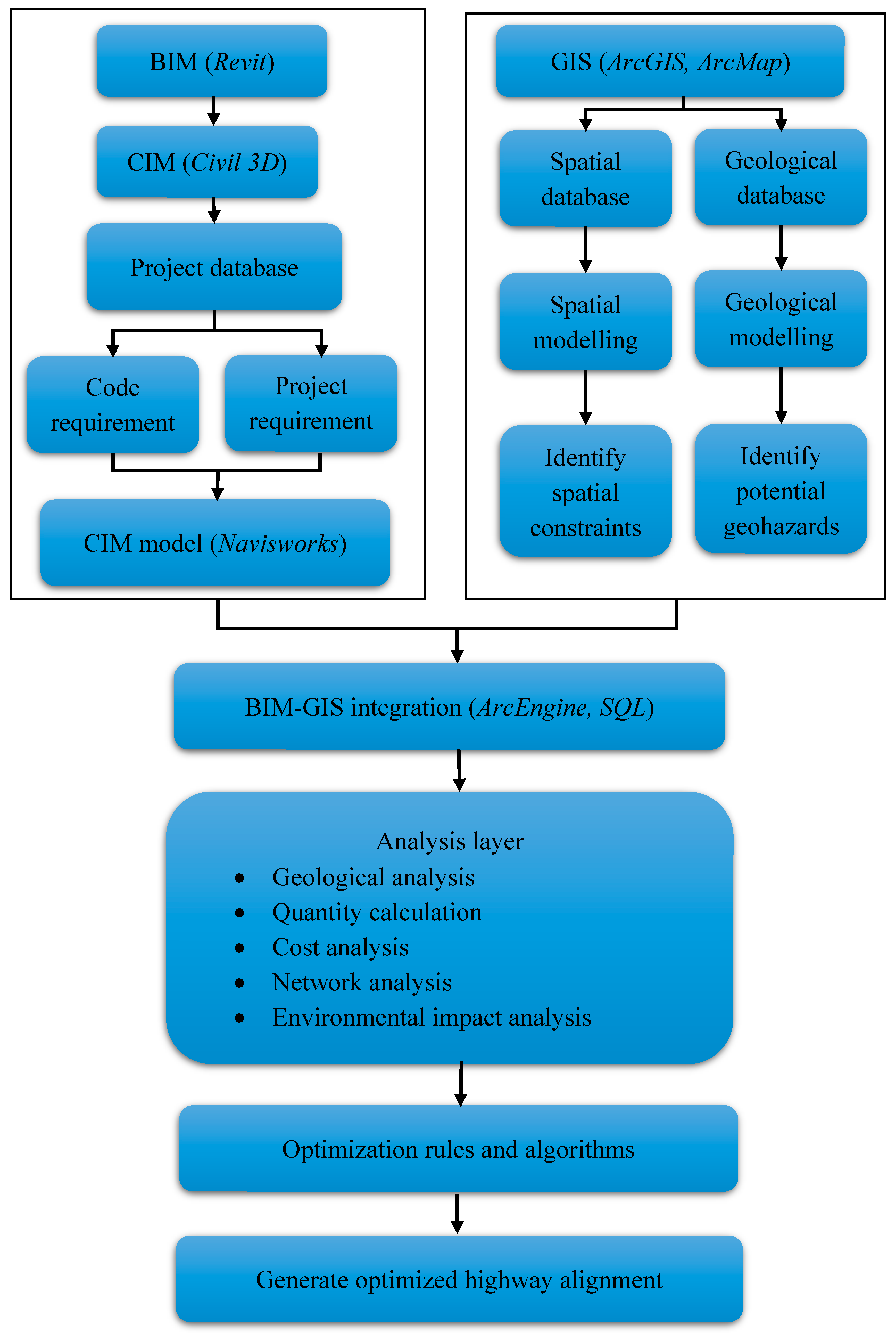
The highway alignment planning process requires information from various sources and reliable analysis to support decision making. As such, the proposed method includes an integrated BIM and GIS model, an analysis module, and an application layer. As shown in
Figure 1, the integrated model extracts the necessary data and information from BIM and GIS to support the analysis module and the optimization layers. The data that were used in the analysis module were retrieved from BIM, GIS, and user input. BIM provides a full range of project information, whereas the GIS provides geodata and information about the surroundings. The retrieved data are then used in the analysis module (e.g., geological analysis, network analysis, cost analysis) that supports the optimization of highway alignments.
The proposed model process is described, as follows. Accurate topographic and geographic data are required, and the design of the alignment of the proposed highway project in BIM, which specifies the grades, is necessary. Subsequently, the design information of the highway is exported into the GIS model to form a new model. The new 3D model is used to analyse the geotechnical structure to provide several alignment options. Finally, the selection process of the alignments is performed according to GAs. If modification is required, the changes to the highway are transferred back to the BIM model. The use of the integrated BIM and GIS models minimizes human interference in data input and all of the data can be structurally stored in order to facilitate customized analytical functions. To facilitate the highway planning and design process, BIM can be used to obtain a detailed quantity take-off of the proposed project and GIS is used to support a wide range of analysis functions.
3.1. The Integrated BIM-GIS Model
A novel integrated BIM and GIS model is proposed in this study based on semantic web technologies. A series of processes is required to that end. First, an IFC ontology is developed to describe the hierarchy structure of BIM objects, their properties, and relationships. Additionally, GIS ontology is constructed by first converting the data to GML and then transforming the GML data into RDF/OWL. Second, ontology matching is performed by using Graph Matching for Ontologies (GMO). These BIM and GIS ontologies are first transferred into RDF bipartite graphs, and GMO is adopted to compare the structural similarities between the BIM and GIS ontologies. The similarity matrix is assigned initial values and the iteration proceeds until 1:1 mapping in the similarity matrix is achieved. This process is conducted by Python. Third, RDF is formalized as BIM and GIS ontologies are merged; at this step, the most important task is the RDF conversion of the merged ontologies while using Java or API. Finally, SPARQL is used to manipulate and retrieve RDF data. The result of a query can be represented as XML, RDF, and CSV. The result is also the format supported by semantic webs, such as Turtle, N-TRIPLE, and JSON-LD. A fully integrated BIM-GIS RDF graph is obtained.
3.1.1. Conceptualizing IFC and CityGML
Web ontology language (OWL) is used to generate the application ontology. Application ontology represents the semantics of a specific application domain, which can be used to define the relevant concepts for a particular application (e.g., BIM and GIS) [
47]. Semantic web technologies usually use description logic to structurally represent the application domain by defining the relevant concepts that can specify the properties of objects in the domain [
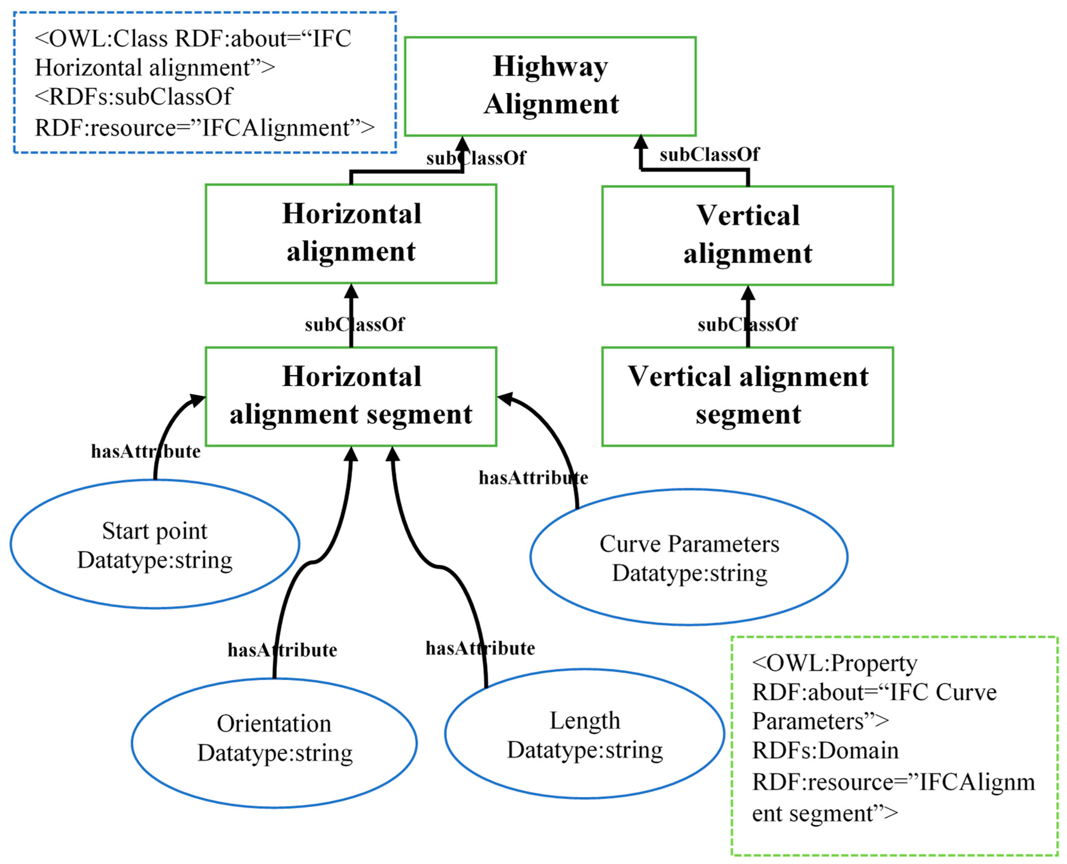
48]. There are two types of concepts: primitive concepts that represent the classes of the IFC domain and defined concepts that define the subclasses of primitive ones [
47]. Hence, the IFC classes at the top of the hierarchical structure of the ontology are defined as primitive concepts. For example, IFC Horizontal alignment is defined as a primitive concept, comprising a subclass of IFC Highway alignment. A Horizontal alignment segment that is a subclass of Horizontal alignment in IFC schema is designated a defined concept. The properties of the concept are displayed in
Figure 2.
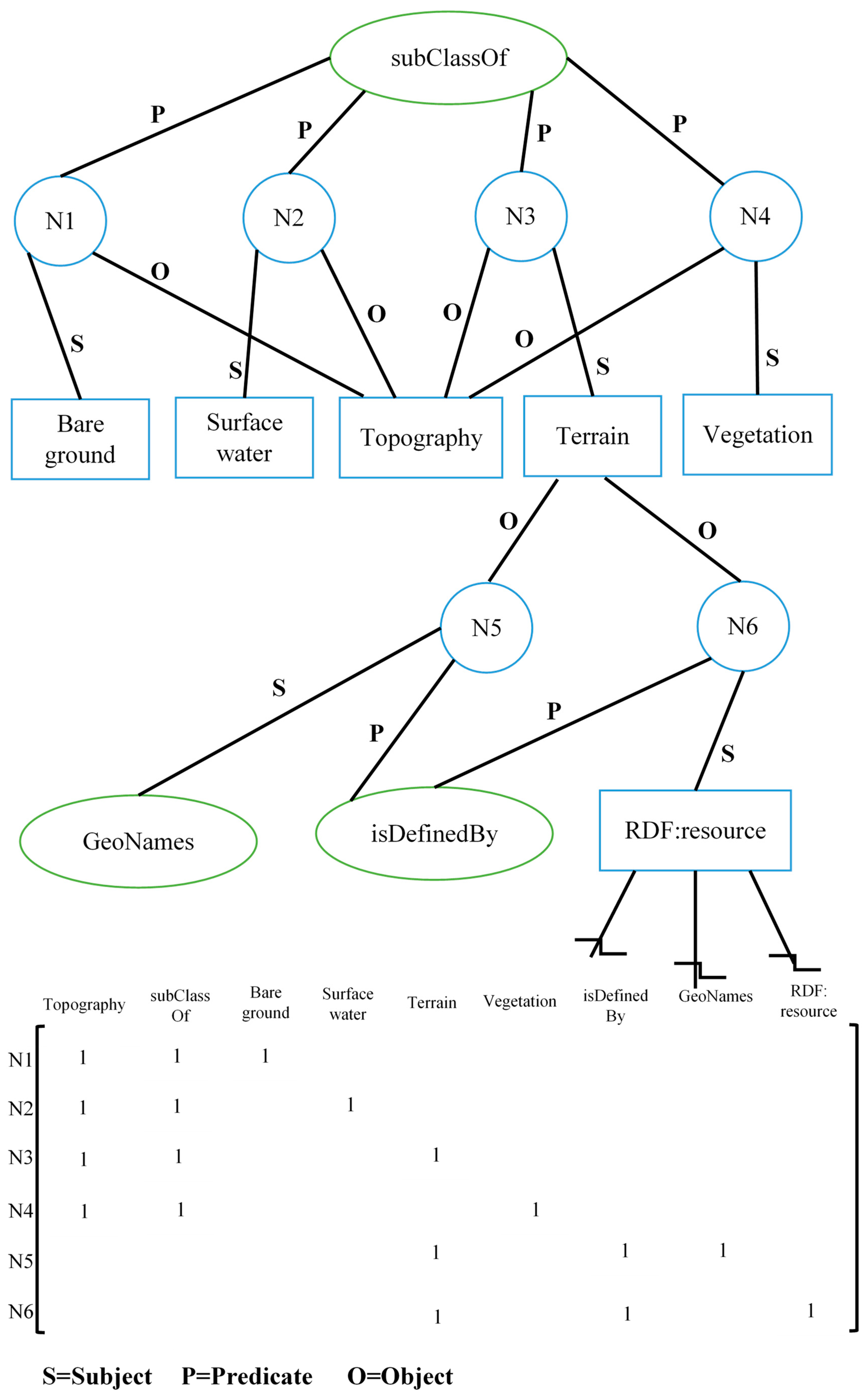
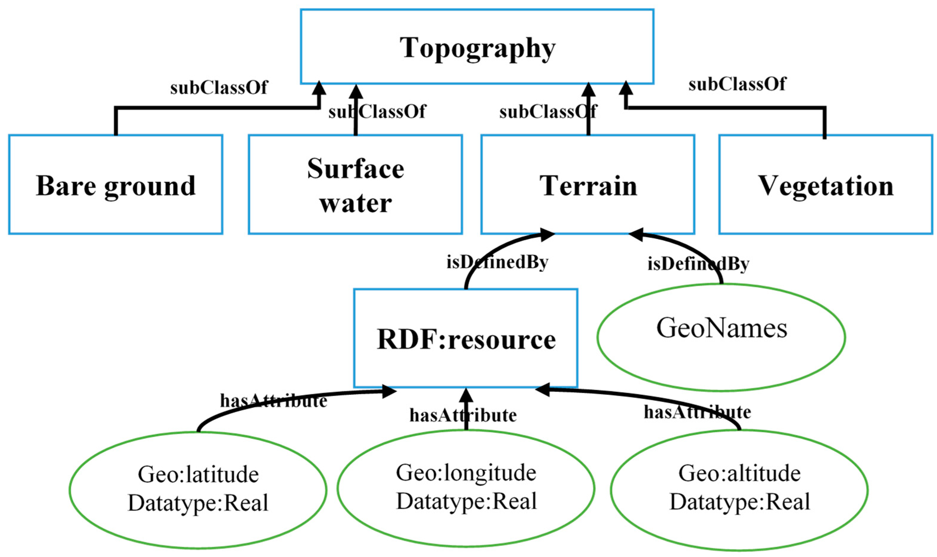
As RDF provides the logical meaning of data, it is an excellent tool for interchanging data between the BIM and GIS systems. In the AEC industry, GIS is usually used to perform geospatial analyses in order to retrieve information regarding the site’s topography and to produce a geo-referenced dataset. A GIS database is a set of relations (tables), including several attributes. Semantic web technology utilizes description logic to represent predicates between different classes. A relation is grouped into tuples that possess the same attributes. It can be defined as an OWL: Class. All of the attributes related to the relation can be defined as properties.
Figure 3 presents an example of such conversion, where a relational database is first transformed into GML and then RDF.
3.1.2. Ontology Matching
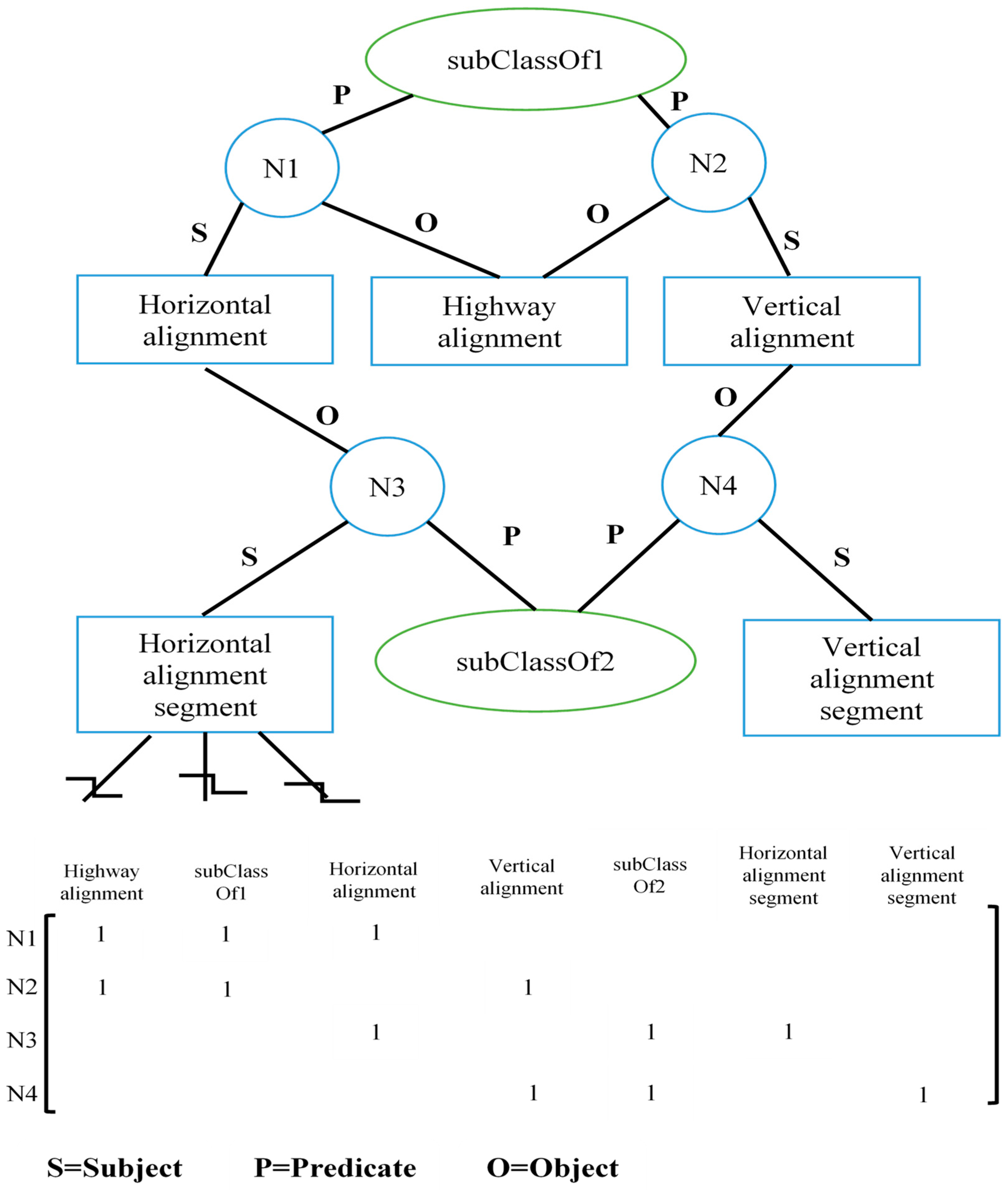
In this step, ontology matching is used to bridge the gap between BIM-ontology and GIS-ontology graphs. Ontology matching plays a key role in the integration between semantic web applications that use different ontologies [
49]. Structural similarity is important in ontology matching. Graph Matching for Ontologies (GMO) is used to measure the structural similarities in this study. The Python is used to implement the GMO. In the GMO approach, the ontologies are converted to bipartite graphs, and then the structural similarities are measured between graphs. The GMO process includes several steps. First, BIM-ontology and GIS-ontology graphs are transformed into RDF bipartite graphs, respectively, as shown in
Figure 4 and
Figure 5. The details of which can be referenced in [
50]. Subsequently, BIM-ontology and GIS-ontology graphs are coordinated while using coordination rules because the two ontologies represent heterogeneous data. Third, matrix representations for BIM ontology and GIS ontology are set up. Afterwards, initial values in similarity matrices are set and convergence precision is defined. Finally, an iteration step is run until 1:1 mapping is achieved in a similarity matrix. The result identifies the correspondences between BIM and GIS.
3.1.3. RDF Formalization
Semantic web queries cannot access the data in BIM and GIS, as BIM- AND GIS-AUTHORING tools do not support them. Hence, IFC data must be transformed to XML data that enables users to query and access data at any time. At this step, BIM and GIS ontologies are transformed into the formal standard ontology language RDF. For example, each IFC entity is represented as the subject in RDF, identified as an OWL:Class, and an RDF: is used to describe the subject. An RDF: subClassOf property is used to indicate that an IFC entity is a subclass of another entity.
3.1.4. Data Querying
SQL is part of SPARQL that is used for RDF graphs. SQL is a query language that enables the semantic web to retrieve and manipulate data stored in the models. The results can provide formats that are supported by the semantic web, including Turtle, N-TRIPLE, NSON-LD, and RDF. This provides an integrated view where applications can access a database that is one integrated knowledge base and one semantic schema. By using SPARQL, the integration of BIM and GIS is obtained, which is a gully integrated BIM-GIS RDF graph, including a set of data with unified geometries, and complementary properties and relationships.
Figure 6 shows the process of integration between BIM and GIS.
3.2. Analysis Module
The proposed method utilizes several fundamental analysis tools from both BIM and GIS to create mathematical solutions for highway alignment planning. These important analysis tools include geological analysis, network analysis, and cost analysis. Geological analysis aims to identify the potential hazards in the project area. Geological analysis is necessary in highway planning and design. For example, when potential hazards are identified, the analysis results can be used to determine the potentially impacted areas and subsequent reinforcement activities. The network analysis tool can plan a route from one point to another in a given network. The BIM data can be retrieved to compute the costs that were incurred in highway alignments planning.
3.2.1. Geological Analysis
The proposed model incorporates geotechnical planning into infrastructural design and thus increases collaboration in order to avoid misunderstanding between the two parties. During the analysis process, the potential geohazards are identified and mitigated or avoided; geological information of the site is presented vividly. This helps engineers to conduct additional analysis and helps in the design of the proposed highway project and related structural works. Geotechnical analysis may lead to several required changes in highway design. These changes are then transferred back to the BIM model. This analysis provides efficient and effective screening of the area of concern and it enables a reasonable view of the risks of the overall area.
Figure 7 shows an example of geological analysis.
Landslide
Prior to construction, a detailed geotechnical analysis of the site is required to identify the landslide risks, because they are one of the most common and serious geological hazards. GIS can be used to predict landslide risk by incorporating information about landscape, geologic origin, and weather conditions. Further analysis, which considers additional information, such as maximum rainfall, average annual rainfall, and historic landslides, can predict the potential degree of landslide for the area.
Seismic Hazards
Due to the damage that resulted from recent large earthquakes, significant efforts are needed to develop refined seismic design procedures for highways [
51]. The possibility of soil liquefaction after quakes should also be considered. In addition, the bearing capacity of the underlying soil may be exceeded after an earthquake, which leads to embankment sliding and crack openings on the highway surface.
Based on the geographical and geological information of the region, a potential area for earthquakes and active faults was identified and selected. From historical records of earthquakes, higher magnitudes were selected for further seismic analysis. After seismic analysis, the liquefaction results of the selected points were generated, which can provide users with additional knowledge of the site that can help them to develop solutions to alleviate or avoid any seismic hazard.
3.2.2. Socio-Economic and Environmental Impacts
The construction of a new highway project may greatly impact human activities or environmentally sensitive areas (e.g., historic areas, forests, and wetlands) in the project area and it may even result in increased levels of noise and air pollution. Generally, these types of impacts are the essential issues in modern highway construction. Thus, these impacts should be considered during highway alignment planning. Detailed information about environmental issues associated with highway construction can be found in [
52].
3.2.3. Cut and Fill Calculations
Cut and fill cost accounts for nearly 25% of the total project cost [
53]. Owing to the complexity of cut and fill calculations, given the limitations of the BIM model it is essential to adopt GIS technology in the calculations [
54]. The proposed model that integrates BIM and GIS is used to carry out cut and fill calculations. Highway geometric information in BIM includes road shape, cross-section, centrelines, elevation, curbs, and embankments, while information, such as triangle co-ordinates and group, geographical and geological reference, soil type, and terrain data can be accessed in the GIS model. The data in BIM and GIS are stored in the IFC and GML format, respectively. Semantic web technology allows for the integration to be combined in the same platform. The quantity calculations of cut and fill are based on the existing topographical elevation in the GIS model. The earthwork simulation aims to minimize the earthwork by balancing the cut and fill operation.
In the highway project, vertical alignment is based on the centreline of the road; thus, the centreline is regarded as the reference line. Centreline elevation occasionally represents the topography of the entire cross-section in terms of earthwork balancing. The term “optimal centreline elevation” represents a centreline elevation, where the cut and fill are balanced within the cross-section. The main idea of this method is to make earthwork optimization possible in terms of cut-fill balancing and earthwork minimization. Equation (1) shows the mathematical representation of the method.
where
is the volume of cross-sectional cut areas;
is the volume of cross-sectional fill areas; n is the number of cross-sectional cut areas; and, m is the number of cross-sectional fill areas.
3.3. Optimization Layer
In the highway alignment planning phase, the general practice is to identify several alignment options and choose the optimal option that is based on the multiple rules. Economic considerations are one of the most influential factors in highway projects [
55]. In some cases, mitigating the risks of individual hazards may increase the vulnerability to another hazard. An economic highway alignment may be more vulnerable to geohazards. The highway design should aim to optimize the overall risk and cost and efficiently and effectively carry this out.
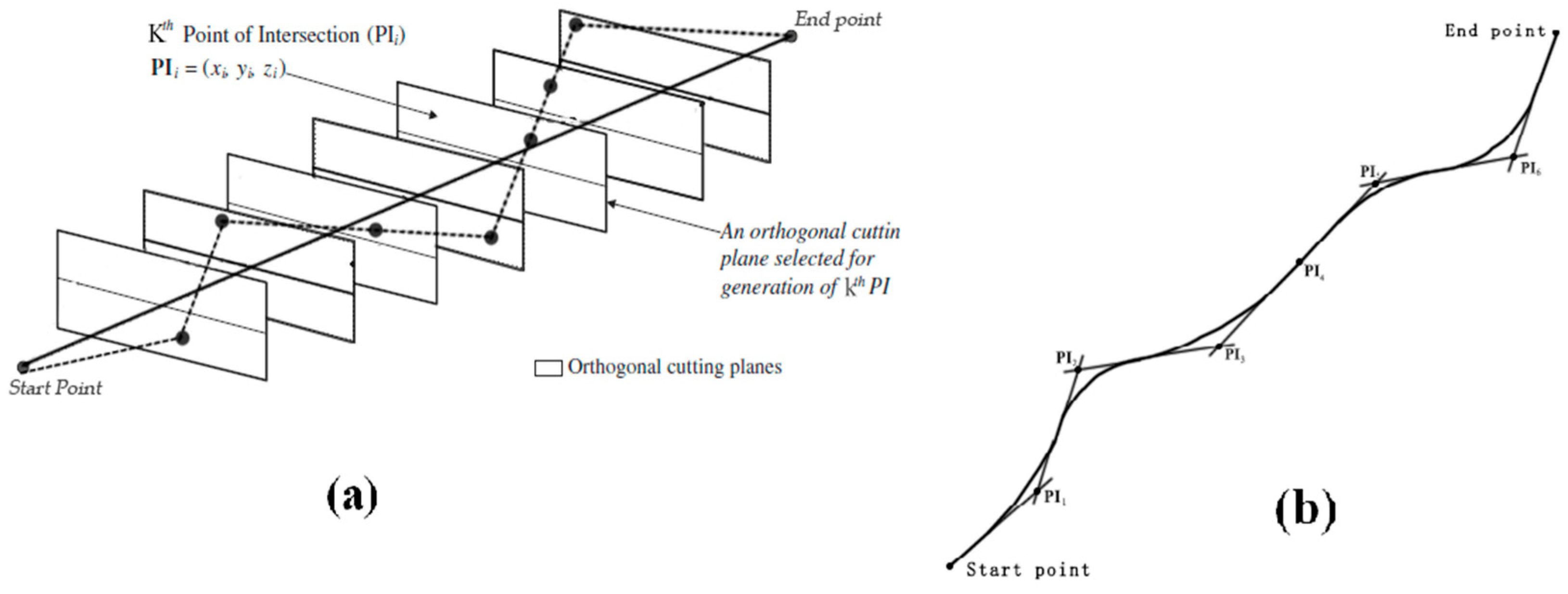
In the highway alignment selection process, a highway alignment is defined by the project requirements, such as tangents, curves, connecting transition curve sections, and graded tangents. The configuration of these factors can be determined by set points of intersections (PIs). Thus, the production of a highway alignment can determine its corresponding series of points. GAs were previously used for highway alignment optimization [
56]. GAs are suitable for optimization problems with several local optima and they fit to parallel processing. In these specified GAs, the problem (highway alignment optimization) is considered as the environment and a set of possible solutions to the proposed problem is regarded as the population. Each alignment in the population is referred to as a chromosome and each chromosome has a set of genes that are defined by the coordinates of points of intersections, as shown in
Figure 8. It should be noted that the points of intersections are not independent of each other, because once a coordinate of one important point is changed, the alignment configuration at another important point may change. A set of variables to the alignment alternative is produced at every generation of search. The variables represent the coordinates of PIs along the alignment alternative in the search area. A floating-point scheme enables the representation of the coordinate values. In general, the coordinate of PI indicates as (
). For an alignment, including
n PIs, the encoded chromosome consists of 3
n genes. According to [
57], the chromosome can be expressed in Equation (2).
where
is chromosome, (
) is the coordinate of the
ith PI, for all
i = 1,
,
n and
is the
ith gene, for all
i = 1,
,
n.
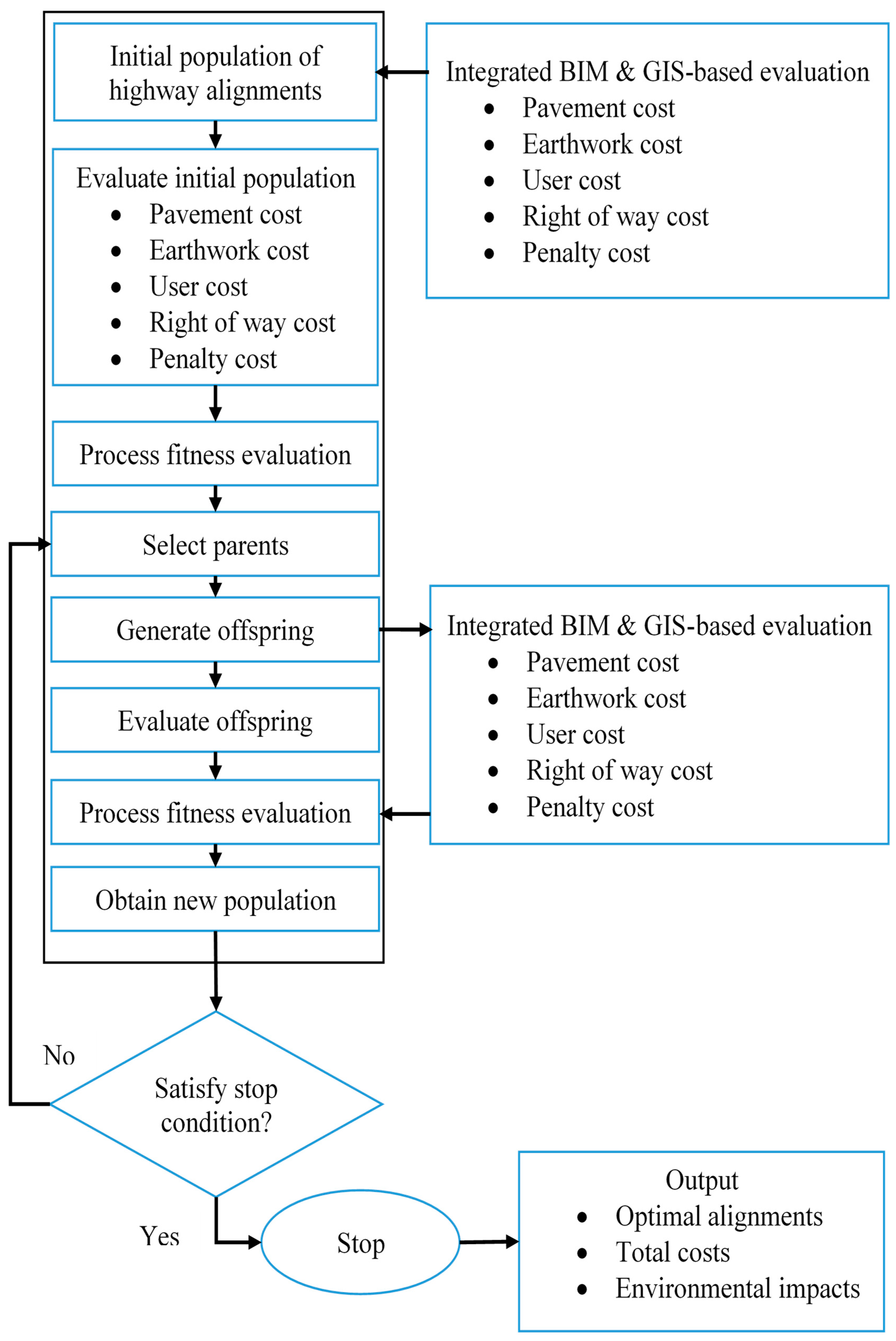
The initial coordinates of PIs are set at the beginning of GAs optimization. During the GAs optimization process, the coordinates are reformed as more-fitted members take the place of old ones by using a selection scheme. Subsequently, the more-fitted members are reserved and they have the chance to create offspring via genetic recombination. At every generation in GAs, the coordinates are passed to the integrated BIM+GIS model to calculate the total cost. This process continues through successive generations until the improvement of objective function becomes negligible. Based on the finding of [
52], the data between GAs and the integration model is enabled by using dynamic link libraries.
Figure 9 shows the optimization process.
Several optimization algorithms are available, such as GAs, network optimization, enumeration, calculus of variations, dynamic programming, numerical research, and linear programming. Among these, the six approaches other than GAs have some essential disadvantages for highway alignment optimization, in which cost functions are implicitly noisy. GAs have critical distinctions relative to other algorithms, as they: (1) search within a population rather than a single point; (2) work with the encoding of parameter sets rather than parameters themselves; (3) adopt decisive information (objective function) rather than auxiliary or derivatives knowledge; and, (4) use probabilistic rules rather than deterministic rules [
58]. Despite these benefits, it should be noted that GAs are not always suitable for all problems, but they can be regarded as an effective approach for quickly finding near-optimal solutions.
3.3.1. Cost Terms in Objective Function
The objective function that was used in this study can be written, as shown in Equation (3).
where
is total cost;
is pavement cost;
is earthwork cost;
is right-of-way cost;
is user cost;
is penalty cost; and,
are decision variable factors.
Equation (4) expresses the pavement cost in this study
where
is the pavement cost,
is the unit pavement cost,
is the length of the highway, and
is the road width.
User cost is can be seen as a length depend cost, as expressed in Equation (5).
where
is user cost;
is unit length-dependent cost; and,
L is the length of road.
The earthwork cost in this study is expressed in Equation (6)
where
is the earthwork cost,
is the unit cutting cost per cubic meter,
is the unit filling cost per cubic meter,
is the transportation cost for transferring one cubic meter of earth to a landfill, and
is the transportation cost for transferring one cubic meter of earth from a borrow pit.
Equation (7) expresses the right-of-way cost in this study
where
is the right-of-way cost,
is the unit land cost in
i region, and
is the square meters affected by the highway in
i region.
3.3.2. Penalty Cost
Various types of socio-economic and environmental areas may be within the area of a new highway project, such as farmland, forest cover, commercial, and residential. The proposed alignment should affect these areas as minimally as possible. In the GIS model, maps containing a variety of geographic data can be used to evaluate the proposed alignment by overlaying on the maps to estimate its impact on the area. Each structure and property in the project area, their corresponding attributes, and their sensitivity to the proposed alignment can be comprehensively assessed in the GIS model. This plays an important role in defining MaxC and calculating the penalty costs. Hence, the affected areas can be calculated for the evaluated alignment. Once the affected areas of the alignment exceed their maximum allowable limit, a penalty cost would be applied to the excess area. Moreover, the penalty cost can also be used in a case where the proposed alignment does not meet the specified project requirements, such as the minimum curve length or angles. Equation (8) expresses the penalty cost.
where
is the significant penalty cost for passing through an extremely environmentally sensitive area,
is the unit cost of the
k environmentally sensitive area that was taken by the alignment,
is the square meter of the
k environmentally sensitive area taken by the alignment, and
is the maximum allowable square meters of the
k environmentally sensitive area that was taken by the alignment.
4. Case Study
4.1. Project Information
The DuAn highway construction project is an important part of highway networks in Guizhou Province, which is located in the southwest part of China. The total length of the project is 282.9 km and the total project cost is 44.63 billion Yuan. The design speed is set at 100 kph. Several factors complicate the project: (1) the natural conditions are harsh; (2) the layout of the route is heavily impacted by existing structures such as railways, bridges, and pipelines; and, (3) the selection of design planning is difficult. Moreover, the project area is within a seismically active region, where a high-intensity earthquake could damage the highway. Seismic shaking can also lead to soil liquefaction and subsequent damage to the highway surface. A seismic hazard analysis was performed on the project site to decide the seismic loads. The construction activities consisted of excavation, subbase, base, subgrade, embankment, surface, drainage, and slope protection. Earthwork excavation and backfill, highway subbase and surface, slope protection, and water drainage were the major tasks in the work package.
4.2. Data from Both BIM and GIS Tools
In this study, Autodesk Civil 3D was adopted as a BIM software application, while ArcMap was utilized as a GIS software application. First, the BIM model of highway elements is required to be defined based on the element classes. Civil 3D software enables the creation of multiple object catalogs. In the BIM model, IFC entities in an EXPRESS schema were used for addressing the geometry, relationships, and attributes of objects. Subsequently, the EXPRESS schema was converted into an OWL. The ontologies were developed to define the classes and relationships of the objects. The IFC schema has primarily concentrated on building entities, such as foundations, walls, windows, and doors. For this study, it is necessary to develop additional entities for use in highway planning. Hence, the ontology is indicated as IFCOWL ontology (IFC4) [
59], with additional tunnel and infrastructure elements being used in this study.
The user can access the element information by choosing the element command button on the screen. Detailed information regarding the project can then be directly obtained from the BIM model, which automatically quantifies specific project information (e.g., length and width of the highway) as soon as the project is modelled in Civil 3D. Readily available BIM-based libraries of the unit cost for the highway objects would enhance the applicability and effectiveness of the proposed method in terms of real-world projects. From the BIM model, the highway pavement cost and user cost can be calculated based on road length and width, which is calculated using Equations (4) and (5).
Table 1 presents the descriptive attributes of the three highway alignments.
Having developed the project model, the next step is to model project site topography model with the GIS module and integrate the highway project and site model together into a single environment. Given the significant amount of geographical data involved, there is great potential in using GIS in highway alignment planning. The application of GIS in this case study is intended to identify the optimal alignment by exploring the information regarding the project’s surroundings. The information about the project’s surroundings was modelled in ArcMap, and a CityGML schema was used for addressing the objects, relationships, and attributes. Subsequently, the CityGML schema has also to be converted into an OWL representation. The topographic information regarding the project’s surroundings is given in the GIS module.
In the third step, Python was used to identify similar concepts for both OWL representations by creating an OWL mapping that contains the similarities of IFC and CityGML. Afterwards, the IFC data and CityGML data were linked. It is possible to utilize semantic web technologies, like the query language SPARQL, which enables querying the CityGML model for some elements that were described in the related IFC model, such as “select Class: ifc: IfcHorizontalalignment to get all the segments in the given alignment”, which are not directly described by CityGML, since there is no particular class for it in CityGML.
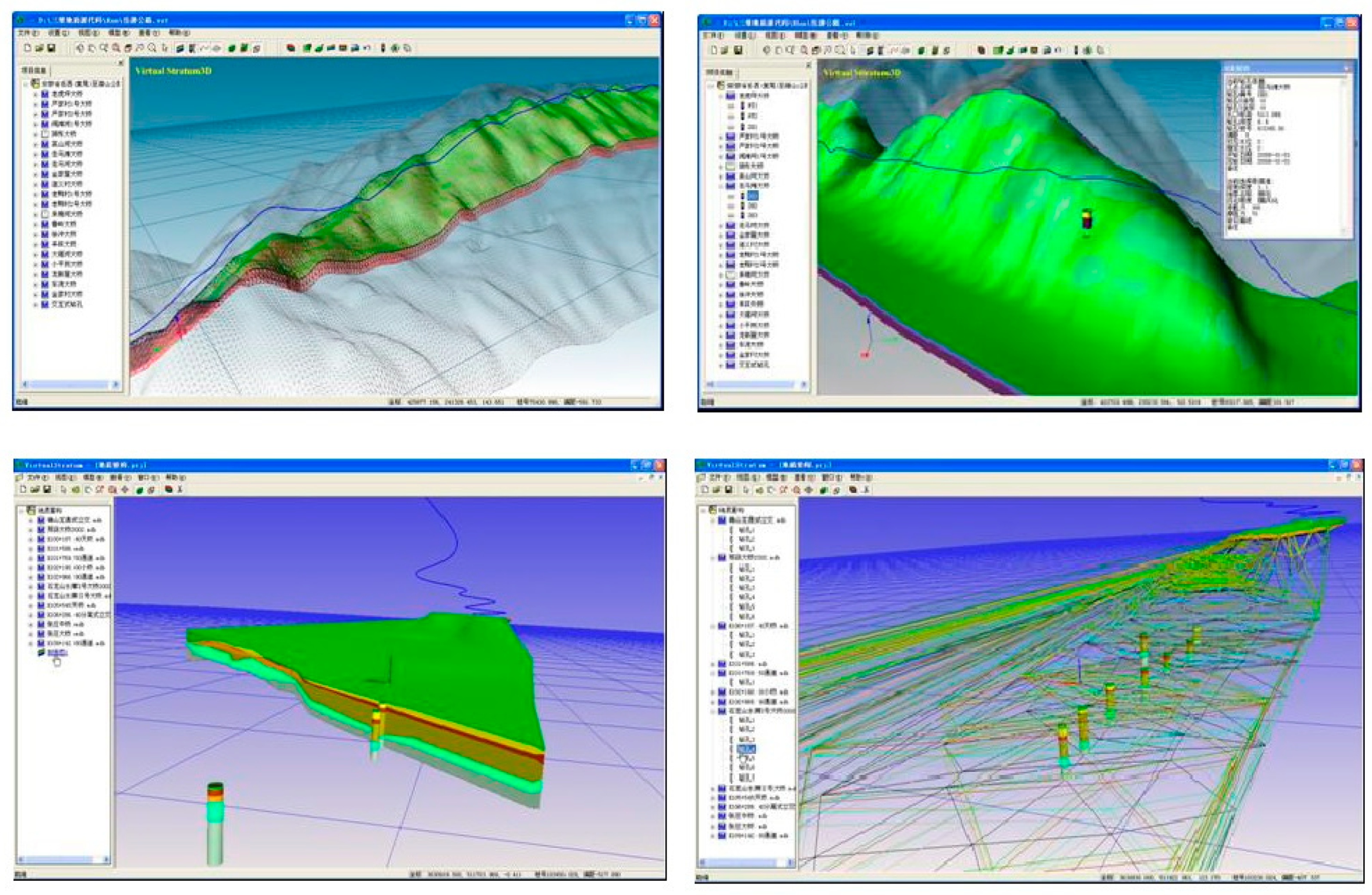
Finally, all of the geometric and geographical information is exported to the GIS module. The 3D visualization model of the highway project and its surroundings is shown. The site topography model is currently used in the visualization of project surroundings. Subsequently, digital elevation models (DEM) can be obtained in GIS to calculate the earthwork costs by using Equation (6). Moreover, the right-of-way cost is estimated according to officially announced average values of the land where the project is proposed to be located. After the unit cost of the land is estimated, the right-of-way cost can be calculated based on Equation (7). In addition, land use analysis can also be carried out in GIS to indicate the environmentally sensitive regions and the square meter of regions that are impacted by the proposed project. To facilitate the highway alignment process, the penalty cost was introduced in the optimum objective function to minimize environmental impact. At this stage, the penalty cost of the proposed highway alignment can be calculated based on Equation (8) in this study.
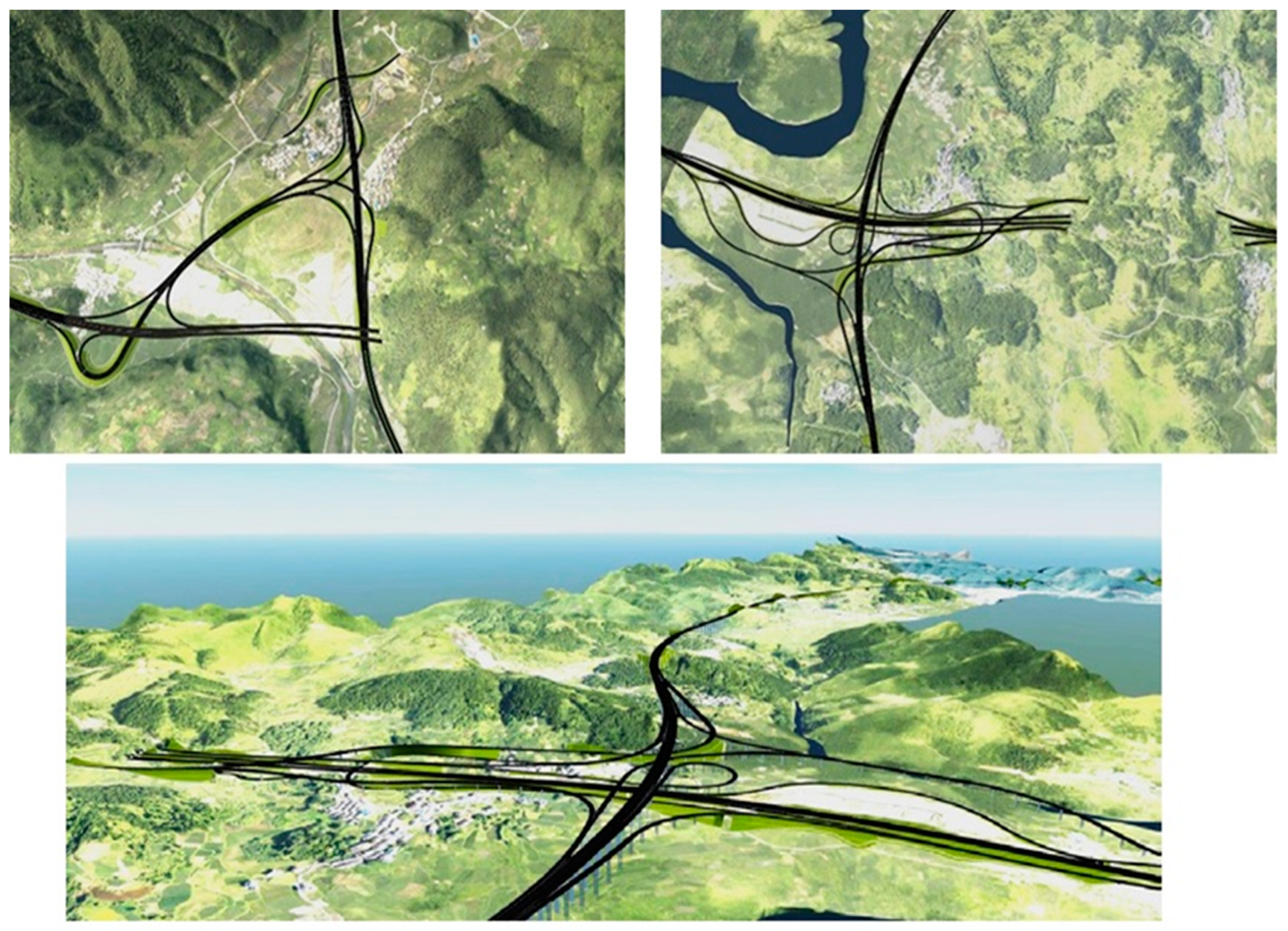
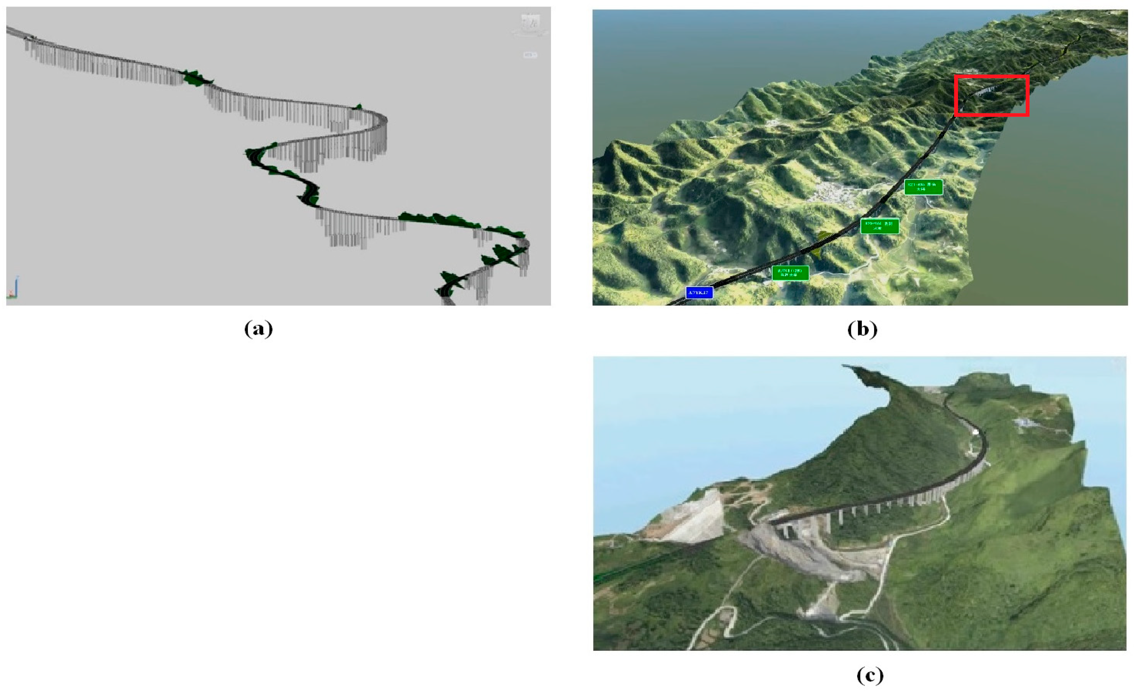
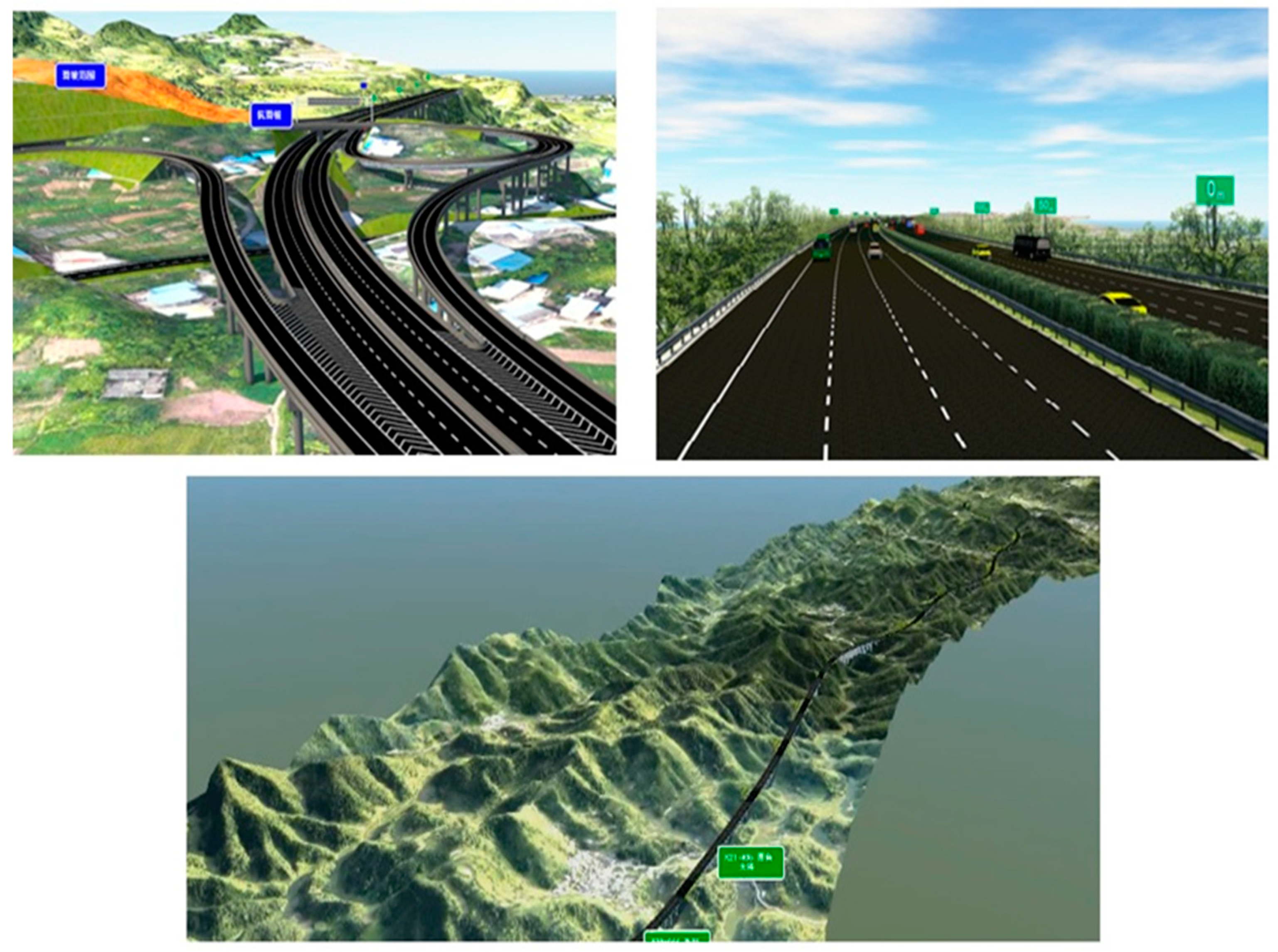
The integrated model can provide three-dimensional visualization of the project with its surroundings, which enables the project participants to better know the project details and its surroundings. The 3D visualized model also facilitates communication among users, and it thus reduces misunderstanding and risks.
Figure 10 presents the 3D visualization model of DuAn highway with its surroundings.
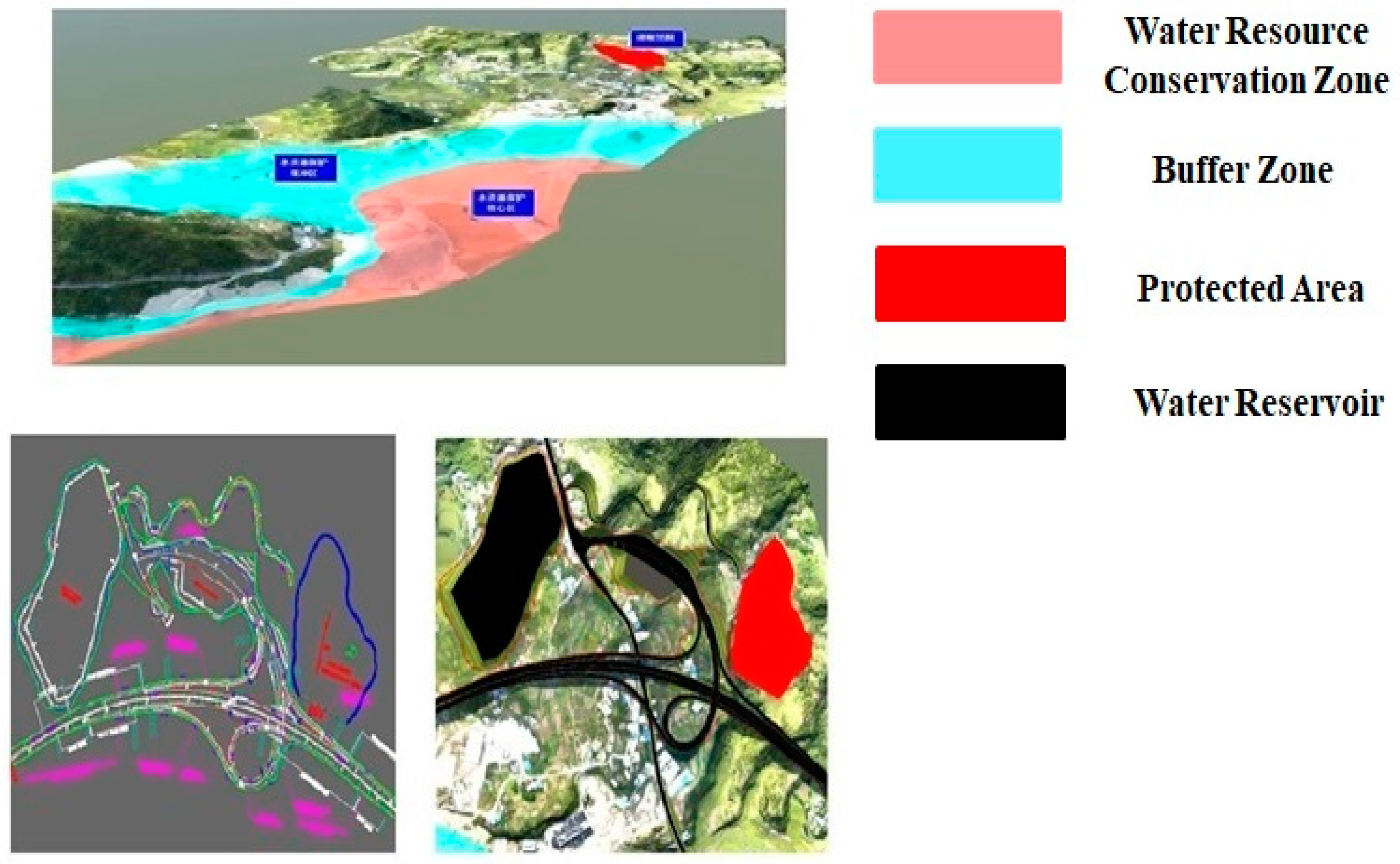
4.3. Geographical and Environmental Issues
When planning a highway project in a given area, a variety of geographically or environmentally sensitive regions, such as historic districts, forest, wetlands, residential properties, and commercial centers may be encountered. To properly reflect the relevant issues in highway alignment planning, tradeoff values that are associated with different land-use types must be thoroughly considered based on their relative importance since these values may greatly impact the proposed alignment. Hence, the maximum allowable areas that are impacted by the proposed highway (denoted as MaxC) are set based on their relative importance. For example, for areas, such as historical districts, MaxC is set much stricter than for areas like farmland and properties. Historical district area is a protected region that is to be avoided by the proposed alignment in this study. The concept is to keep the highway away from it, while allowing the alignment to pass through the farmland and properties areas while still minimizing its effects on these areas. For this purpose, MaxC of the protected area is set at 0, indicating that the historical district area must not be impacted by the proposed alignment. For other areas, including farmland and properties, MaxC is supposed to be minimized in this study. The geographic maps of the project area are shown in
Figure 11.
Figure 12 shows the environmental analysis of the highway project.
4.4. Optimized Alignment
Genetic algorithms (GAs) was adopted to find the optimal alignment for the highway project. The most used objective function is to minimize the cost. A directional route of the proposed highway project is created by the BIM module, based on the design code and project requirements. Subsequently, this information was transferred to GIS. Recall that, in this case study project, the objective function contains five cost items (
). The environmental impact cost was included, being indicated as a penalty cost. Hence, the optimization process aims to identify a perfect trade-off that minimizes total costs while satisfying the specified project requirements and environmental constraints. An optimized alignment was obtained through 100 generations, as shown in
Figure 13. Its total cost is about CNY 14.96 billion. Its length is 282.9 kilometers, affecting a total farmland area of about 909.53 hectare, a forest area of about 444.9 hectare, a pasture area of about 256.98 hectare, a parkland area of about 58.55 hectare, and residential properties of about 46.14 hectare. No impact on historical districts is found. It should be noted that this does not mean that individual cost items will ultimately be similar. Several alignments may generate a similar total cost, but quite different individual cost items. This indicates that, in the alignment optimization process, an appropriate objective function should be selected to reflect all of the critical highway cost items. This importance will be further examined in the sensitivity analysis regarding changes in the objective function.
5. Analysis and Validation
5.1. Sensitivity Analysis
Sensitivity analysis of optimized alignments with respect to the objective function is performed, which aims to indicate that all of the alignment-sensitive costs should be considered and properly involved in the highway optimization objective function. Three alignments were generated based on three different cost combinations. Each of these used identical variables, except the cost items that were included in the objective function, as follows.
Optimal alignment was generated by using the first cost combination as the objective function, as shown in
Figure 14(a1). It passes through some hazard sensitive areas (e.g., landslides). In addition, its corresponding vertical alignment closely follows ground elevation, except for one significant area of hilly terrain and several small ones that greatly increases the cost of earthworks, as shown in
Figure 14(b1). The results show that the optimization process did not consider the geological conditions and the topography of the area. The objective function in this case does not contain the right-of-way costs, penalty costs, and earthwork costs.
Figure 14(a2) presents the alignment optimized by the second cost combination, which hardly impacts environmental sensitive areas and avoids hazard sensitive areas. However, it is relatively circuitous and it has the longest length among the three alignments. Moreover, its vertical alignment, as shown in
Figure 14(b2), is not optimized, because it significantly differs from the ground profile. These results indicate that the second cost combination does not consider earthwork costs.
Figure 14(a3) presents the optimized alignment that is produced by the third cost combination. The alignment is a straight line, which indicates that it has the shortest distance. Additionally, it avoids most of the hazard and environmentally sensitive areas. Its corresponding vertical alignment closely follows the ground profile, as shown in
Figure 14(b3), which occurred due to simultaneous optimization of horizontal and vertical alignments, while minimizing the costs. These results indicate that all of the major costs associated with optimized alignment planning should be simultaneously considered.
Three alignment alternatives were generated based on different objective functions. Although alignment 1 may have the lowest cost, it is subjected to a greater level of geohazards based on the results from the geological analysis. Moreover, the construction of alignment 1 would exacerbate the environmental sensitivity problem with the surroundings. Alignment 2 nearly avoids all potential geohazards, even those with the highest cost, but it has too many conflicts with existing structures that are based on the 3D visualization model. When considering all of these important factors, alignment 3 is the optimal option.
Table 1 summarizes the cost analysis and environmental impacts of the alignments.
The results indicate that the highway alignment that was determined by the proposed model can avoid disastrous soil structure and geohazards, conform to changes in the terrain, and mitigate the disturbances of existing projects. The earthwork calculation that was assisted by the proposed model also generated accurate results that save costs and time at the construction stage. In addition, the proposed model provides sufficient information that can facilitate the decision-making process. Based on feedback from the project users, they all agreed that the proposed model enabled a quick alignment optimization process with great precision as compared to the conventional manual methods.
5.2. Cost Analysis
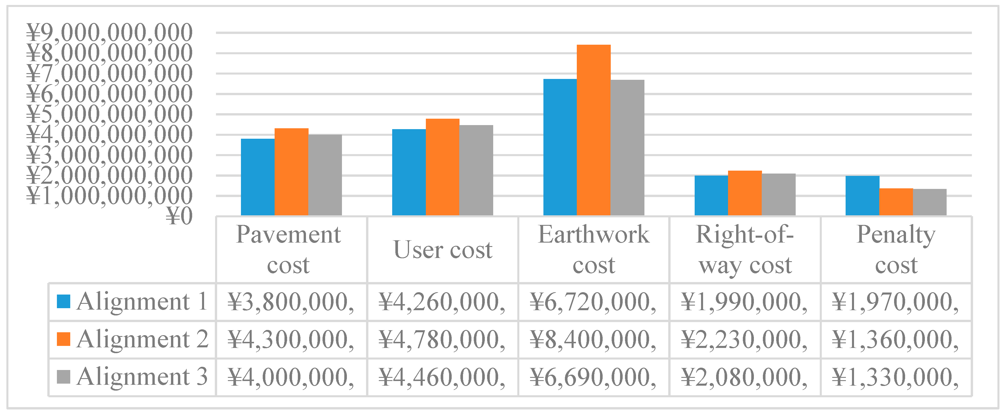
The cost analysis is supposed to identify the costs, including pavement cost, user cost, earthwork cost, right-of-way cost, and penalty cost for each highway alignment alternative. The estimated costs are based on the integrated BIM and GIS model.
Figure 15 shows the costs that are related to each cost item for each alternative. The major cost that is related to this highway alignment planning is the earthwork cost, which is greater than any other single cost. The earthwork costs vary among the alternatives.
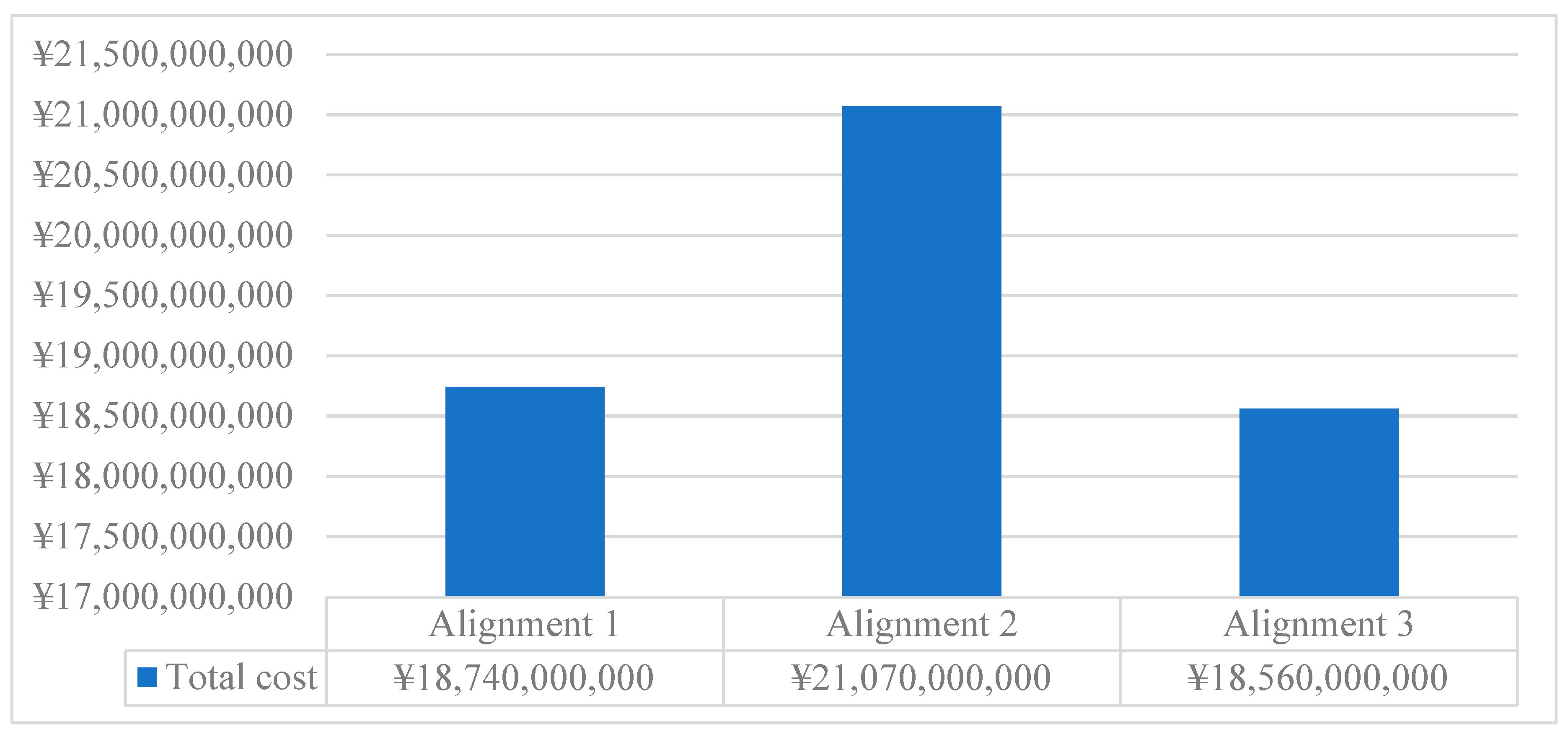
Figure 16 presents the estimated total cost for each highway alignment alternative. Alignment 3 has the lowest estimated cost, at CNY 14.96 billion, followed by Alignment 1 at CNY 15.32 billion. Alignment 2 has the highest estimated total cost of CNY 17.2 billion. Based on the cost analysis, alignment 3 is the optimal alignment.
5.3. Method Validation
The proposed model to integrate BIM and GIS was tested on a real case project. The results indicate that the proposed model can capture all of the information regarding the highway project components and their surroundings. The proposed model provides detailed and vivid information regarding the project and its surroundings in a single environment.
Figure 17 shows the benefits of the proposed method in this case. As can be seen from
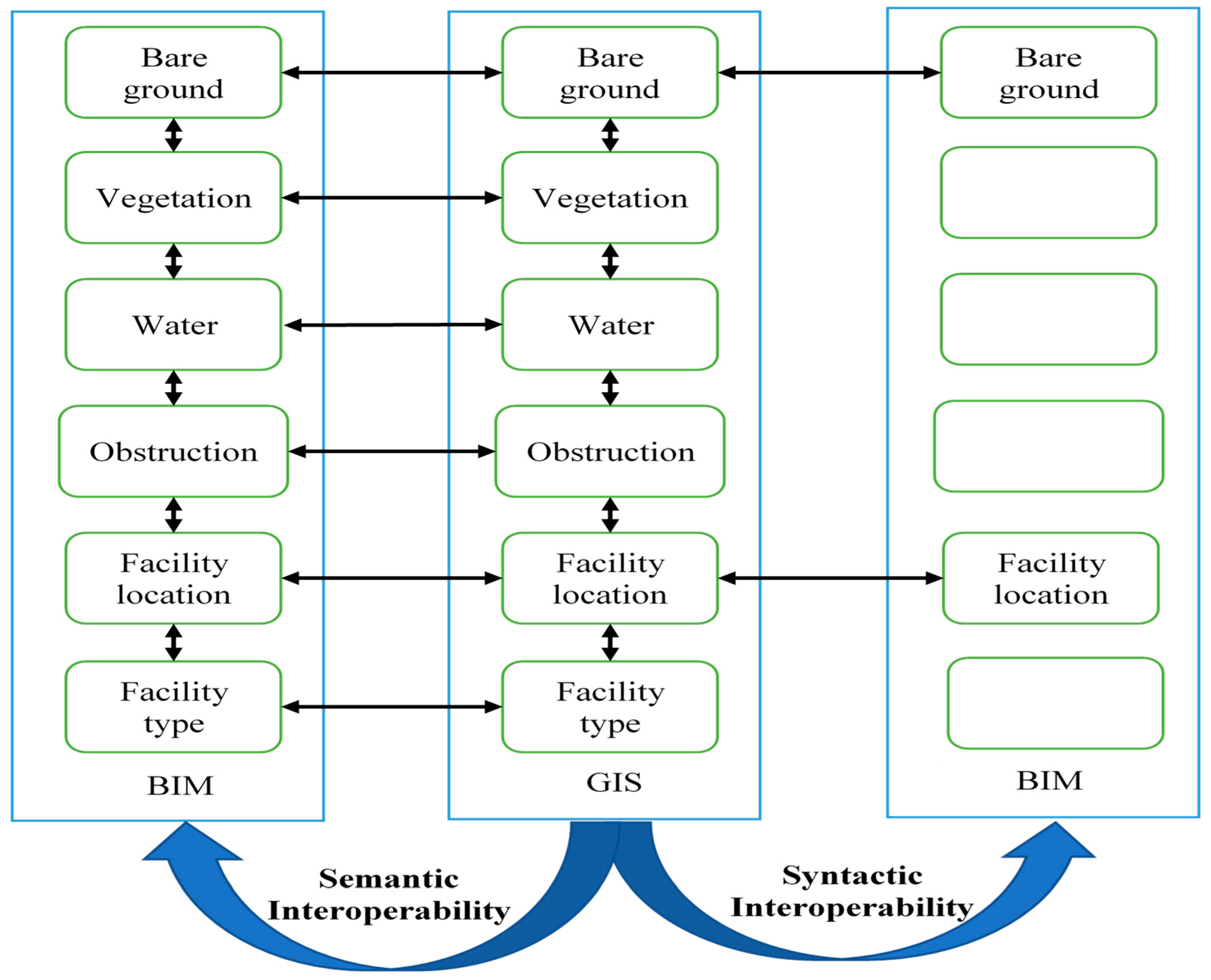
Figure 17, the project details and surroundings all can be shown clearly, which facilitate the highway alignment planning process. This is not a first attempt to combine the advantages of GIS and BIM. However, the proposed integration between the two systems at a semantic level is more advanced than that in the current practices, which enable data interoperability at the syntactic level.
Figure 18 shows the difference between the two integrated methods.
6. Conclusions
Highway alignment planning is typically a complex and time-consuming process. The evaluation of different alignment alternatives is even more time-consuming and it tends to be costly. The proposed model integrates BIM and GIS systems to facilitate this process. The integration of BIM and GIS systems is complex and it includes a large amount of data. Semantic web technologies and ontology were used to facilitate integration.
The proposed model improves the efficiency of the geotechnical and infrastructural planning and design process. The proposed model closes the gap in information flow between highway design and geotechnical analysis and it also provides a 3D highway model. Moreover, the adoption of semantic web technologies allows for data exchanges to occur between BIM and GIS systems and thus increases data interoperability. Furthermore, the optimization algorithms (GAs) are used to select the optimal alignment. The proposed model is able to concurrently maximize the control of geohazards and minimize project costs.
The automation process of the proposed model provides an opportunity to identify optimal alignment in a timely way. The use of the proposed model in a real highway project demonstrated its potential for application in the industry. As both the BIM and GIS systems continue to develop in the civil infrastructure sector, the proposed model could be shared and it becomes more acceptable in the industry.
This study makes four contributions. First, the integration of BIM and GIS systems enables data exchange in two ways that significantly improves data interoperability. Subsequently, GAs are applied to conduct multiple alignment simulations. Second, the proposed model provides geological analysis to indicate highway alignment design to avoid or mitigate potential hazards. Third, the automated process of multiple alignment alternative analysis provides an opportunity to identify an optimal option in a timely way. Finally, the proposed model provides a virtual environment, where changes in decisions can be made more easily and cost-effectively.
In this study, the integration model only applies to the highway project, though it may also be helpful for other projects, such as pipelines, tunnels, and bridges. In further studies, the proposed model may also apply to other horizontal projects (e.g., pipelines), and the proposed model can also be integrated with other advanced technologies to be used in construction site layout or building fire evacuation.
Author Contributions
Conceptualization, L.Z. and Z.L.; methodology, J.M.; software, Z.L.; validation, L.Z., Z.L.; resources, L.Z.; writing—original draft preparation, L.Z.; writing—review and editing, J.M.; visualization, Z.L.
Funding
This research was funded by National Key Research and Development Program of China, grant number 2018YFF0300300, Beijing University of Technology, grant number 2018JG08704, and The APC was funded by the both grants.
Acknowledgments
The authors would like to thank the Beijing University of Technology for its support through the research project. The authors would like to thank China Communications Construction, China Railway Group Limited, China State Construction Engineering Corporation, and China Association of Technology Entrepreneurs for providing data to conduct this research. In addition, I would like to thank all practitioners who contribute in this project.
Conflicts of Interest
The authors declare no conflict of interest.
Abbreviations
| AEC | Architectural Engineering and Construction |
| API | Application Programming Interface |
| BIM | Building Information Modelling |
| CIM | Civil Information Modelling |
| CSV | Comma Separated Values |
| DEM | Digital Elevation Model |
| Gas | Genetic Algorithms |
| GIS | Geographic Information System |
| GML | Geography Markup Language |
| GMO | Graph Matching Ontologies |
| IFC | Industry Foundation Class |
| MaxC | Maximum allowable area can be taken by the project |
| OWL | Web Ontology Language |
| PIs | Points of Intersections |
| RDF | Resource Description Framework |
| SQL | Structural Query Language |
| XML | eXtensible Markup Language |
References
- Costin, A.; Adibfar, A.; Hu, H.; Chen, S.S. Building inforamtion modelling (BIM) for transportation infrastructure-Literature review, application, challenges, and recommendations. Autom. Constr. 2018, 94, 257–281. [Google Scholar] [CrossRef]
- Cylwik, E.; Dwyer, K. Virtual Design and Construction in Horizontal Infrastructure Projects. Eng. News-Rec. 2012. Available online: https://www.enr.com/ (accessed on 28 December 2018).
- Karan, E.P.; Irizarry, J. Extending BIM interoperability to preconstruction operations using geospatial analyses and semantic web services. Autom. Constr. 2015, 53, 1–12. [Google Scholar] [CrossRef]
- Wang, J.F.; Zhang, T.L.; Fu, B.J. A measure of spatial stratified heterogeneity. Ecol. Indic. 2016, 67, 250–256. [Google Scholar] [CrossRef] [Green Version]
- Mignard, C.; Nicolle, C. Merging BIM and GIS using ontologies application to urban facility management in ACTIVe3D. Comput. Ind. 2014, 65, 1276–1290. [Google Scholar] [CrossRef]
- R&S Market Research. Global Geographic Information System (GIS) Market Expected to Grow at 11% CAGR during 2015–2020; R&S Market Research: New York, NY, USA, 2016. [Google Scholar]
- Parsons, R.L.; Frost, J.D. Interactive analysis of spatial subsurface data using GIS-based tool. J. Comput. Civ. Eng. 2000, 14, 215–222. [Google Scholar] [CrossRef]
- Anumba, C.; Dainty, A.; Ison, S.; Sergeant, A. The Utilisation of GIS in the Construction Labour Market Planning Process; Emerald Group Publishing Limited: Bingley, UK, 2008. [Google Scholar]
- Su, X.; Andoh, A.R.; Cai, H.; Pan, J.; Kandil, A.; Said, H.M. GIS-based dynamic construction site material layout evaluation for building renovation projects. Autom. Constr. 2012, 27, 40–49. [Google Scholar] [CrossRef]
- Bansal, V.K. Use of GIS and topology in the identification and resolution of space conflicts. J. Comput. Civ. Eng. 2011, 25, 159–171. [Google Scholar] [CrossRef]
- Su, X.; Zhang, L.; Andoh, A.R.; Cai, H. In GIS-based buffering for construction workspace management. In Proceedings of the International Conference of ASCE on Construction Research Congress, West Lafayette, IN, USA, 21–23 May 2012; pp. 1252–1261. [Google Scholar]
- Andoh, A.; Su, X.; Cai, H. A Framework of RFID and GPS for Tracking Construction Site Dynamics. In Proceedings of the ASCE International Conference on Construction Research Congress, West Lafayette, IN, USA, 21–23 May 2012; pp. 818–827. [Google Scholar]
- Ko, C.H. 3D-Web-GIS RFID location sensing system for construction objects. Sci. World J. 2013, 2013, 217972. [Google Scholar] [CrossRef] [PubMed]
- Bansal, V.K.; Pal, M. Construction projects scheduling using GIS tools. Int. J. Constr. Manag. 2011, 11, 1–18. [Google Scholar] [CrossRef]
- Migliaccio, G.C.; Zandbergen, P.; Martinez, A.A. Empirical comparison of methods for estimating location cost adjustments factors. J. Manag. Eng. 2013, 31, 1–10. [Google Scholar] [CrossRef]
- Shrestha, K.; Shrestha, P. A GIS-enabled cost estimation tool for road upgrade and maintenance to assist road asset management systems. In Proceedings of the ASCE Conference on Construction Research Congress, Reston, VA, USA, 19–21 May 2014; pp. 1239–1248. [Google Scholar]
- Bansal, V.K. Application of geographic information systems in construction safety planning. Int. J. Proj. Manag. 2011, 29, 66–77. [Google Scholar] [CrossRef]
- Jia, N.; Xie, M.; Chai, X. Development and implementation of a GIS-based safety monitoring system for hydropower station construction. J. Comput. Civ. Eng. 2012, 26, 43–53. [Google Scholar] [CrossRef]
- Kim, H.; Orr, K.; Shen, Z.; Moon, H.; Ju, K.; Choi, W. Highway alignment construction comparison using object-oriented 3D visualization modeling. J. Constr. Eng. Manag. 2014, 140, 1–12. [Google Scholar] [CrossRef]
- Shou, W.; Wang, J.; Wang, X.; Chong, H.Y. A comparative review of building information modelling implementation in building and infrastructure industries. Arch. Comput. Methods Eng. 2015, 22, 291–308. [Google Scholar] [CrossRef]
- Costin, A. A New Methodology for Interoperability of Heterogeneous Bridge Information Models. Ph.D. Thesis, Georgia Institute of Technology, Atlanta, GA, USA, 2016. [Google Scholar]
- Cheng, C.P.; Lu, Q.; Deng, Y. Analytical review and evaluation of civil information modeling. Autom. Constr. 2016, 67, 31–47. [Google Scholar] [CrossRef]
- Volk, R.; Stengel, J.; Schultmann, F. Building Information Modelling (BIM) for existing buildings-literature review and future needs. Autom. Constr. 2014, 38, 109–127. [Google Scholar] [CrossRef]
- Vacca, G.; Quaquero, E.; Pili, D.; Brandolini, M. Integrating BIM and GIS Data to Support the Management of Large Building Stocks. ISPRS Int. Arch. Photogramm. Remote. Sens. Spat. Inf. Sci. 2018, XLII-4, 647–653. [Google Scholar] [CrossRef]
- Sadeghi-Niaraki, A.; Varshosaz, M.; Kim, K.; Jung, J.J. Real world representation of a road network for route planning in GIS. Expert Syst. Appl. 2011, 38, 11999–12008. [Google Scholar] [CrossRef]
- Zhu, J.; Wright, G.; Wang, J.; Wang, X. A cititcal review of the integration of Geographic Information System and Building Information Modelling at the data level. ISPRS Int. J. Geo-Inf. 2018, 7, 66. [Google Scholar] [CrossRef]
- Deng, Y.; Cheng, J.C.P.; Anumba, C. Mapping between BIM and 3D GIS in different levels of detail using schema mediation and instance comparison. Autom. Constr. 2016, 67, 1–21. [Google Scholar] [CrossRef]
- De Laat, R.; van Berlo, L. Integration of BIM and GIS: The development of the citygml GeoBIM extension. In Advances in 3D Geo-Information Sciences; Kolbe, T.H., König, G., Nagel, C., Eds.; Springer: Berlin/Heidelberg, Germany, 2011. [Google Scholar]
- El-Mekawy, M.; Östman, A.; Hijazi, I. An evaluation of IFC-CityGML unidirectional conversion. Int. J. Adv. Comput. Sci. Appl 2012, 3, 159–171. [Google Scholar] [CrossRef]
- Costa, G.; Sicilia, Á.; Lilis, G.; Rovas, D.; Izkara, J. A comprehensive ontologies-based framework to support retrofitting design of energy-efficient districts. In Proceedings of the European Conference on Product and Process Modelling (ECPPM), Limassol, Cyprus, 9–11 September 2016. [Google Scholar]
- Alreshidi, E.; Mourshed, M.; Rezgui, Y. Factors for effective BIM governance. J. Build. Eng. 2017, 10, 89–101. [Google Scholar] [CrossRef] [Green Version]
- Horrocks, I. Ontologies and the semantic web. Commun. ACM 2008, 51, 58–67. [Google Scholar] [CrossRef]
- Ali, M.; Mohamed, Y. A method for clustering unlabeled BIM objects using entropy and TF-IDF with RDF encoding. Adv. Eng. Inform. 2017, 33, 154–163. [Google Scholar] [CrossRef]
- Jelokhani-Niaraki, M.; Sadeghi-Niaraki, A.; Choi, S.-M. Semantic interoperability of GIS and MCDA tools for environmental assessment and decision making. Environ. Model. Softw. 2018, 100, 104–122. [Google Scholar] [CrossRef]
- Guarino, N.; Oberle, D.; Staab, S. What is an ontology? In Handbook on Ontologies; Staab, S., Studer, R., Eds.; Springer: Berlin, Germany, 2009; pp. 1–17. [Google Scholar]
- Song, Y.; Wang, X.; Tan, Y.; Wu, P.; Sutrisna, M.; Cheng, J.C.P.; Hampson, K. Trends and Opportunities of BIM-GIS Integration in the Architecture, Engineering and Construction Industry: A Review from a Spatio-Temporal Statistical Perspective. Int. J. Geo-Inf. 2017, 6, 397. [Google Scholar] [CrossRef]
- Suchocki, M. BIM for infrastructure: Integrating spatial and model data for more efficient contextual planning, design, construction and operation. In Building Information Modelling (BIM) in Design, Construction and Operations; Mahdjoubi, L., Brebbia, C.A., Laing, R., Eds.; WIT PRESS: Boston, MA, USA, 2015. [Google Scholar]
- Kim, H.; Chen, Z.; Cho, C.-S.; Moon, H.; Ju, K.; Choi, W. Integration of BIM and GIS: Highway Cut and Fill Earthwork Balancing. In Proceedings of the 2015 International Workshop on Computing in Civil Engineering, Austin, TX, USA, 21–23 June 2015; pp. 468–474. [Google Scholar]
- Barazzetti, F.; Banfi, F. BIM and GIS: When parametric modellign meets geospatial data. ISPRS Ann. Photogramm. Remote. Sens. Spat. Inf. Sci. 2017, 4, 1–8. [Google Scholar] [CrossRef]
- OECD. Optimization of Road Alignment by the Use of Computers; Organization of Economic Cooperation and Development: Paris, France, 1973. [Google Scholar]
- Chapra, S.C.; Canale, R.P. Numerical Methods for Engineers; McGraw-Hill: New York, NY, USA, 2006. [Google Scholar]
- Fwa, T.F. Highway vertical alignment analysis by dynamic programming. J. Transp. Res. Board 1989, 1239, 2–3. [Google Scholar]
- De Smith, M.J. Determination of gradient and curvature constrained optimal paths. Comput.-Aided Civ. Infrastruct. Eng. 2006, 21, 24–38. [Google Scholar] [CrossRef]
- Lee, Y.; Tsou, Y.R.; Liu, H.L. Optimization method for highway horizontal alignment design. J. Transp. Eng. 2009, 135, 217–224. [Google Scholar] [CrossRef]
- Jong, J.C. Optimizing Highway Alignments with Genetic Algorithms. Ph.D. Thesis, University of Maryland, College Park, MD, USA, 1998. [Google Scholar]
- Kang, M.W.; Schonfeld, P.; Yang, N. Prescreening and repairing in a genetic algorithm for highway alignment optimization. Comput.-Aided Civ. Infrastruct. Eng. 2009, 24, 109–119. [Google Scholar] [CrossRef]
- Karan, E.P.; Irizarry, J.; Haymaker, J. BIM and GIS integration and interoperability based on semantic web technology. J. Comput. Civ. Eng. 2016, 30, 1–11. [Google Scholar] [CrossRef]
- Studer, R.; Grimm, S.; Abecker, A. Semantic Web Services: Concepts, Technologies, and Applications; Springer: Berlin, Germany, 2007. [Google Scholar]
- Hu, W.; Jian, N.; Qu, Y.; Wang, Y. GMO: A graph matching for ontologies. In Proceedings of the K-CAP Workshop on Integrating Ontologies, Banff, AB, Canada, 2 October 2005; pp. 41–48. [Google Scholar]
- Hayes, J.; Gutierrez, C. Bipartite graphs as intermediate model for RDF. In Proceedings of the 3rd International Semantic Web Conference, Hiroshima, Japan, 7–11 November 2004; pp. 47–61. [Google Scholar]
- Yen, W.P.; Fallon, J.D.O.; Cooper, J.D.; Higgins, M. FHWA/MCEER Seismic Research for Transportation Structures. In Proceedings of the Structures Congress 2001, Washington, DC, USA, 21–23 May 2001. [Google Scholar]
- Jha, M.K. A Geographic Information Systems-Based Model for Highway Design Optimization; University of Maryland: College Park, MD, USA, 2000. [Google Scholar]
- Hare, W.L.; Koch, V.R.; Lucet, Y. Models and algorithms to improve earthwork operations in road design using mixed integer linear programming. Eur. J. Oper. Res. 2011, 215, 470–480. [Google Scholar] [CrossRef]
- Nassar, K.; Hosny, O.; Aly, E.A.; Osman, H. Developing an Efficient Algorithm for Balancing Mass-Haul Diagram. In Proceedings of the International Workshop on Computing in Civil Engineering, Miami, FL, USA, 19–22 June 2011; pp. 396–404. [Google Scholar]
- Goktepe, A.B.; Lav, A.H. Method for optimizing earthwork considering soil properties in the geometric design of highways. J. Surv. Eng. 2004, 130, 183–190. [Google Scholar] [CrossRef]
- Jha, M.K.; Schonfeld, P. A highway alignment optimization model using geographic information systems. Transp. Res. Part A Policy Pract. 2004, 38, 455–481. [Google Scholar] [CrossRef]
- Jha, M.K.; Schonfeld, P.; Jong, J.C.; Kim, E. Intelligent Road Design; WIT Press: South Hampton, UK, 2006. [Google Scholar]
- Goldberg, D.E. Genetic Algorithms in Search, Optimization, and Machine Learning; Addison-Wesley Reading: Reading, MA, USA, 1989. [Google Scholar]
- Vilgertshofer, S.; Amann, J.; Willenborg, B.; Borrmann, A.; Kolbe, T.H. Linking BIM and GIS models in infrastructure by example of IFC and CityGML. In Proceedings of the ASCE International Workshop on Computing in Civil Engineering 2017, Seattle, WA, USA, 25–27 June 2017; pp. 133–141. [Google Scholar]
Figure 1.
Overview of the proposed approach.
Figure 1.
Overview of the proposed approach.
Figure 2.
A building information modelling (BIM) entity representation as an resource description framework (RDF) graph and web ontology language (OWL) Classes.
Figure 2.
A building information modelling (BIM) entity representation as an resource description framework (RDF) graph and web ontology language (OWL) Classes.
Figure 3.
A geographic information science (GIS) entity representation as an RDF.
Figure 3.
A geographic information science (GIS) entity representation as an RDF.
Figure 4.
RDF bipartite graph and matrix representation of the BIM ontology example.
Figure 4.
RDF bipartite graph and matrix representation of the BIM ontology example.
Figure 5.
RDF bipartite graph and matrix representation of the GIS ontology example.
Figure 5.
RDF bipartite graph and matrix representation of the GIS ontology example.
Figure 6.
The BIM and GIS integration process.
Figure 6.
The BIM and GIS integration process.
Figure 7.
An example of geological analysis.
Figure 7.
An example of geological analysis.
Figure 8.
(a) A series of PIs; (b) geometric specification of typical horizontal alignment.
Figure 8.
(a) A series of PIs; (b) geometric specification of typical horizontal alignment.
Figure 9.
The optimization process.
Figure 9.
The optimization process.
Figure 10.
Three-dimensional (3D) model of DuAn highway with its surroundings.
Figure 10.
Three-dimensional (3D) model of DuAn highway with its surroundings.
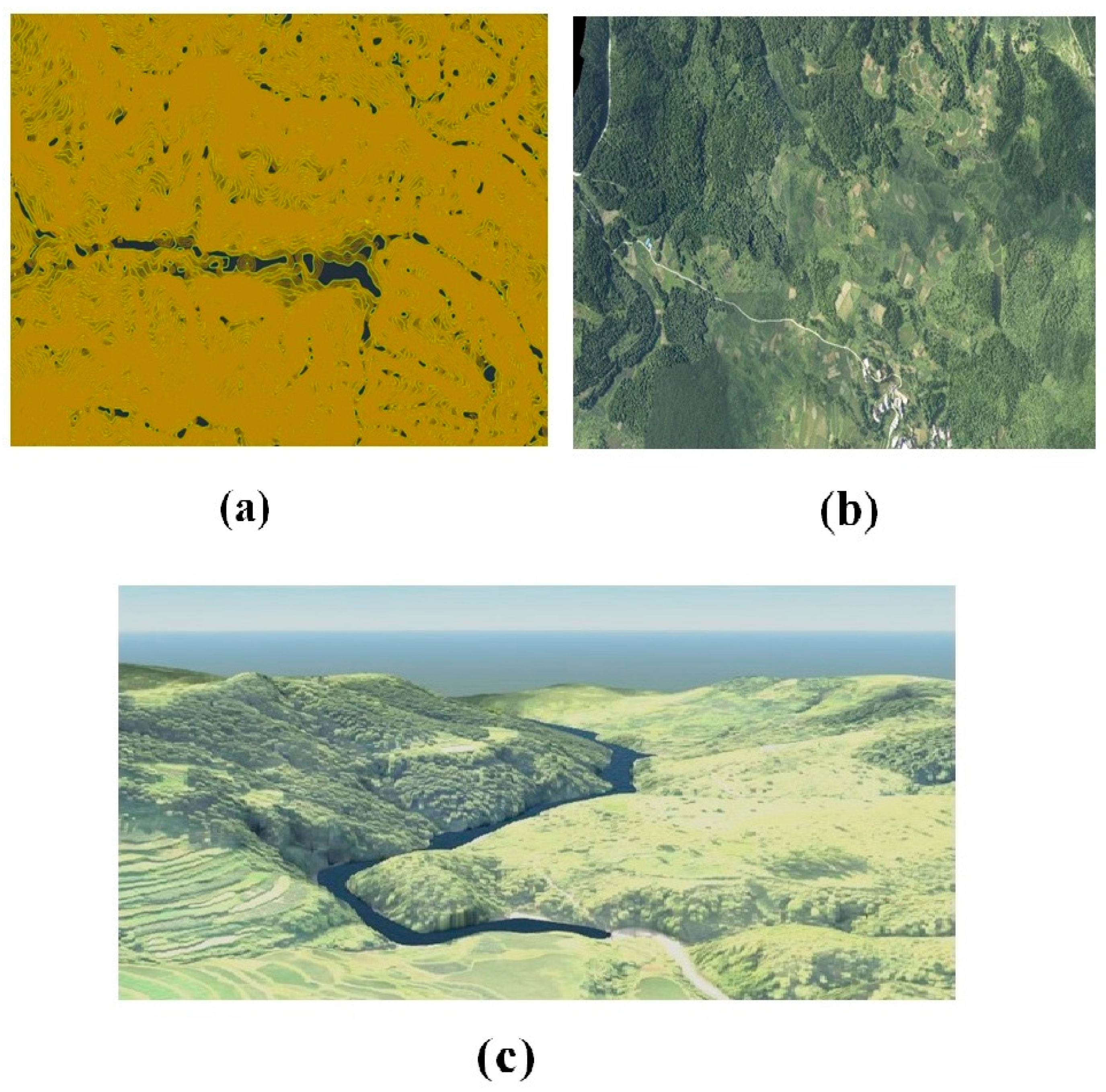
Figure 11.
(a) 1:2000 geographic map; (b) The actual geographic map generated by photogrammetry; and, (c) 3D map.
Figure 11.
(a) 1:2000 geographic map; (b) The actual geographic map generated by photogrammetry; and, (c) 3D map.
Figure 12.
Environmental analysis of the highway project.
Figure 12.
Environmental analysis of the highway project.
Figure 13.
Optimized alignment for DuAn highway.
Figure 13.
Optimized alignment for DuAn highway.
Figure 14.
(a1) The optimal horizontal alignment generated based on the first cost combination; (b1) the vertical alignment generated based on the first cost combination; (a2) the optimal horizontal alignment generated based on the second cost combination; (b2) the optimal vertical alignment generated based on the second cost combination; (a3) the optimal horizontal alignment generated based on the third cost combination; (b3) the optimal vertical alignment generated based on the third cost combination
Figure 15.
Cost items for the three alignment alternatives.
Figure 15.
Cost items for the three alignment alternatives.
Figure 16.
Total cost comparison of three alignment alternatives.
Figure 16.
Total cost comparison of three alignment alternatives.
Figure 17.
(a) The project in BIM environment; (b) the overview of the project in the integrated system; (c) the enlarged section (the squared part in (b)) of the project in the integrated system.
Figure 17.
(a) The project in BIM environment; (b) the overview of the project in the integrated system; (c) the enlarged section (the squared part in (b)) of the project in the integrated system.
Figure 18.
Comparison between the proposed method and current practices for data interoperability between BIM and GIS.
Figure 18.
Comparison between the proposed method and current practices for data interoperability between BIM and GIS.
Table 1.
The summary of cost and environmental impacts of the alignment alternatives.
Table 1.
The summary of cost and environmental impacts of the alignment alternatives.
| Alternatives | Highway Alignment 1 | Highway Alignment 2 | Highway Alignment 3 |
|---|
| Length (km) | 270.6 | 303.1 | 282.9 |
| Total Costs (Billion Yuan) | 18.74 | 21.07 | 18.56 |
| Pavement cost | 3.80 | 4.30 | 4.00 |
| User cost | 4.26 | 4.78 | 4.46 |
| Right-of-way cost | 1.99 | 2.23 | 2.08 |
| Penalty cost | 1.97 | 1.36 | 1.33 |
| Earthwork cost | 6.72 | 8.40 | 6.69 |
| Geological conditions | Low | Low | Low |
| Impacted historical districts (m2) | 0 | 0 | 0 |
| Impacted farmland (hm2) | 1358 | 1204 | 909.53 |
| Impacted forest (hm2) | 508.5 | 487 | 444.9 |
| Impacted pasture (hm2) | 290.1 | 276.9 | 256.98 |
| Impacted parkland (hm2) | 80.4 | 60.5 | 58.55 |
| Impacted industrial facilities (No.) | 0 | 0 | 0 |
| Business displacements (No.) | 0 | 0 | 0 |
| Residential use land (hm2) | 70.6 | 42.8 | 46.14 |
| Cut (m3) | 6312.1 × 104 | 5400.3 × 104 | 5962.45 × 104 |
| Fill (m3) | 5649.3 × 104 | 7366.61 × 104 | 5666.61 × 104 |
| Pavement (m2) | 4026.78 × 103 | 4510.42 × 103 | 4209.82 × 103 |
© 2019 by the authors. Licensee MDPI, Basel, Switzerland. This article is an open access article distributed under the terms and conditions of the Creative Commons Attribution (CC BY) license (http://creativecommons.org/licenses/by/4.0/).


